IFIC/01$-$02

FTUV/01$-$0117

The vector form factor of the pion from unitarity

and analyticity: a model–independent approach

A. Pich and J. Portolés

Departament de Física Teòrica, IFIC, CSIC – Universitat de València,

Edifici d’Instituts d’Investigació, Apt. Correus 22085, E–46071 València, Spain

We study a model–independent parameterization of the vector pion form factor that arises from the constraints of analyticity and unitarity. Our description should be suitable up to $\sqrt{s}\simeq 1.2\,\mbox{GeV}$ and allows a model–independent determination of the mass of the $\rho(770)$ resonance, $M_{\rho}=(775.1\pm 0.5)\,\mbox{MeV}$. We analyse the experimental data on $\tau^{-}\rightarrow\pi^{-}\pi^{0}\nu_{\tau}$, in this framework, and its consequences on the low–energy observables worked out by chiral perturbation theory. An evaluation of the two pion contribution to the anomalous magnetic moment of the muon, $a_{\mu}$, and to the fine structure constant, $\alpha(M_{Z}^{2})$, is also performed.

PACS numbers: 13.35.Dx,13.40.Gp,13.65.+i,12.39.Fe

1 Introduction

The hadronic matrix elements of Quantum Chromodynamics (QCD) currents play a basic role in the understanding of electroweak processes at the low–energy regime (typically $E\sim 1\,\mbox{GeV}$). However our poor knowledge of the QCD dynamics at these energies introduces annoying and serious incertitudes in the description and prediction of the processes involved.

To bypass this problem several procedures have been addressed in the literature on this topic. On one side there is a widespread set of models that pretend to describe, in a simplified way, the involved dynamics [1, 2]. While of importance to get a feeling of the entangled physics, the included simplifying assumptions are usually poorly justified and, sometimes, even inconsistent with QCD. Ad hoc parameterizations of the matrix elements have also been extensively used [2, 3]. The problem with this technique is that, while the description of data can be properly accounted for, it is not easy to work out the physics hidden in the parameters.

A more promising and model–independent procedure is the use of effective actions from QCD. At very low energies ($E\ll M_{\rho}$, with $M_{\rho}$ the mass of the $\rho(770)$ resonance) the most important QCD feature is its chiral symmetry that is realized in chiral perturbation theory ($\chi$PT) [4], a perturbative quantum field theory that provides the effective action of QCD in terms of the lightest pseudoscalar mesons. $\chi$PT has a long and successful set of predictions both in strong and electroweak processes [5]. At higher energies ($E\sim M_{\rho}$), resonance chiral theory is the analogous framework [6] where the lightest resonance fields are kept as explicit degrees of freedom. With the addition of dynamical constraints coming from short–distance QCD, resonance chiral theory becomes a predictive model–independent approach to work with.

One of the simplest hadronic matrix elements of a QCD current is the vector pion form factor $F_{V}(s)$ defined through,

$$\langle\,\pi^{+}(p)\,\pi^{-}(p^{\prime})|\,V_{\mu}^{3}\,|\,0\,\rangle\;=\;(p-p^{\prime})_{\mu}\,F_{V}(s)\;\;,$$ (1)

where $s=q^{2}=(p+p^{\prime})^{2}$ and $V_{\mu}^{3}$ is the third component of the vector current associated with the approximate $SU(3)_{V}$ flavour symmetry of the QCD lagrangian. The vector pion form factor drives the hadronic part of both $e^{+}e^{-}\rightarrow\pi^{+}\pi^{-}$ and $\tau^{-}\rightarrow\pi^{-}\pi^{0}\nu_{\tau}$ processes in the isospin limit . There is an extensive bibliography on the study of this form factor that we do not review in detail here.

At very low energies, $F_{V}(s)$ has been calculated in $\chi$PT up to ${\cal O}(p^{6})$ [7, 8]. A successful study at the $\rho(770)$ energy scale has been carried out in the framework of the resonance chiral theory (the effective action of QCD at the resonance region) in Ref. [9]. In this last reference the unitarity and analyticity properties of the vector pion form factor were implemented in order to match the low–energy result at ${\cal O}(p^{4})$ in $\chi$PT with the correct behaviour at the $\rho(770)$ peak. The result is in excellent agreement with the data coming from $e^{+}e^{-}\rightarrow\pi^{+}\pi^{-}$ and $e^{-}\pi^{\pm}\rightarrow e^{-}\pi^{\pm}$ processes. This solution, that includes the $\rho(770)$ contribution only, leaves just one free parameter, $M_{\rho}$, and provides a suitable description of $F_{V}(s)$ up to $\sqrt{s}\sim 1\,\mbox{GeV}$. If we want to be able to extend its validity at higher energies we should take into account other contributions. To achieve this feature, the analyticity and unitarity properties of $F_{V}(s)$, together with the resonance chiral theory, continue to provide a model–independent solution for the vector pion form factor that we analyse, in detail, in this article. The new solution includes two, a priori, unknown parameters in addition to $M_{\rho}$. These parameters happen to be related to the chiral low–energy observables in Ref. [7, 8], the squared charged pion radius, $\langle r^{2}\rangle_{V}^{\pi}$, and the ${\cal O}(s^{2})$ term in the chiral expansion $c_{V}^{\pi}$.

In the next section we construct the vector pion form factor on grounds of its analyticity and unitarity relations. In Section 3 we study the experimental data on $\tau^{-}\rightarrow\pi^{-}\pi^{0}\nu_{\tau}$ with our solution for the pion form factor. By a fitting procedure we determine the values of $M_{\rho}$ and low–energy parameters that tau decay data demand. Section 4 is devoted to analyse the results we have got from the fitting procedure and the consequences on the chiral observables of $\chi$PT. A corresponding evaluation of the two–pion contribution to the hadronic part of the anomalous magnetic moment of the muon and the fine structure constant is collected in Section 5. We present our conclusions in Section 6.

2 Analyticity and unitarity in $F_{V}(s)$

The vector pion form factor $F_{V}(s)$ is an analytic function in the whole complex s–plane, but for the cut along the positive real axis, starting at the lowest threshold $s=4m_{\pi}^{2}$, where its imaginary part develops a discontinuity. This is given by the unitarity condition

$$\mbox{Im}\,F_{V}(s)\,=\,\frac{\displaystyle 1}{\displaystyle 2}\,\sum_{n}\,\int\,d\rho_{n}\,\langle\,\pi^{+}\pi^{-}\,|\,T^{\dagger}\,|\,n\,\rangle\,\langle\,n\,|\,V_{\mu}^{3}\,|\,0\,\rangle\;\;,$$ (2)

where $|n\rangle$ represents on–shell intermediate states and $T^{\dagger}$ is the scattering operator connecting the intermediate state $|n\rangle$ to the final two–pion state. The first allowed intermediate states are $2\pi$, $4\pi$ and $K\overline{K}$. To every intermediate state corresponds a branch point at the value of $s$ equal to the squared sum of masses of the corresponding particles, i.e. $s=(2m_{\pi})^{2}$, $s=(4m_{\pi})^{2}$, and so on. In the elastic region, $s<16m_{\pi}^{2}$, the only intermediate state considered in Eq. (2) is the one with $2\pi$, and Watson final–state theorem [10] relates the imaginary part of $F_{V}(s)$ to the partial wave amplitude $t_{1}^{1}(s)$ for $\pi\pi$ elastic scattering with angular momentum and isospin equal to one. Thus, from Eq. (2),

$$\mbox{Im}\,F_{V}(s+i\varepsilon)\,=\,\sigma_{\pi}\,t_{1}^{1}(s)\,F_{V}(s)^{*}\,=\,e^{i\,\delta_{1}^{1}}\,\sin\delta_{1}^{1}\,F_{V}(s)^{*}\;\;,$$ (3)

where $\sigma_{\pi}=\sqrt{1-4m_{\pi}^{2}/s}$. As $\mbox{Im}F_{V}(s+i\varepsilon)$ is a real quantity, the phase of $F_{V}(s)$ must be $\delta_{1}^{1}(s)$, that is, the phase–shift of the $t_{1}^{1}(s)$ partial wave amplitude. Therefore,

$$\mbox{Im}\,F_{V}(s+i\varepsilon)\,=\,\tan\delta_{1}^{1}\,\mbox{Re}\,F_{V}(s)\;\;.$$ (4)

The analyticity and unitarity properties of $F_{V}(s)$ are accomplished by demanding that the form factor should satisfy a n–subtracted dispersion relation in the form

$$F_{V}(s)\;=\;\sum_{k=0}^{n-1}\,\frac{\displaystyle s^{k}}{\displaystyle k!}\,\frac{\displaystyle d^{k}}{\displaystyle ds^{k}}\,F_{V}(s)|_{s=0}\,+\,\frac{\displaystyle s^{n}}{\displaystyle\pi}\,\int_{4m_{\pi}^{2}}^{\infty}\,\frac{\displaystyle dz}{\displaystyle z^{n}}\,\frac{\displaystyle\tan\delta_{1}^{1}(z)\,\mbox{Re}F_{V}(z)}{\displaystyle z-s-i\varepsilon}\;\;,$$ (5)

where we have used Eq. (4). This integral equation has the known Omnès solution [9, 11]

$$F_{V}(s)\,=\,Q_{n}(s)\,\exp\left\{\,\frac{\displaystyle s^{n}}{\displaystyle\pi}\,\int_{4m_{\pi}^{2}}^{\infty}\,\frac{\displaystyle dz}{\displaystyle z^{n}}\,\frac{\displaystyle\delta_{1}^{1}(z)}{\displaystyle z-s-i\varepsilon}\,\right\}\;\;,$$ (6)

with

$$Q_{n}(s)\,=\,\exp\left\{\,\sum_{k=0}^{n-1}\,\frac{\displaystyle s^{k}}{\displaystyle k!}\,\frac{\displaystyle d^{k}}{\displaystyle ds^{k}}\,\ln F_{V}(s)|_{s=0}\,\right\}\;\;.$$ (7)

Strictly speaking the solution (6) for $F_{V}(s)$ is valid only below the inelastic threshold $(s<16m_{\pi}^{2})$. This is because we have only included the two–pion threshold in the unitarity relation (2). However, the contributions from higher multiplicity intermediate states are suppressed by phase space and ordinary chiral counting.

As in any subtracted dispersion relation like the one given by Eq. (5) there is an interplay between the subtraction constants (polynomial part) and the dispersive integral. By increasing the number of subtractions (correspondingly increasing the power of $z$ in the denominator) we pull in the low–energy part of $\mbox{Im}F_{V}(s)$ in the integrand . Then the values of $\mbox{Im}F_{V}(s)$ in the upper part of the integration are less important. At the same time the information of this high energy region shifts to the increasing number of subtraction constants that are related with the low–energy expansion of the form factor. This situation is reflected in the solution of the integral equation (6). If we know the $\delta_{1}^{1}(s)$ phase–shift only at very low energies, an accurate evaluation of the integral in Eq. (6) would require a high number of subtractions. This exchange of information between high and low energies is, by no means, paradoxical. It is a strict consequence of the fact that, being an analytic function in the complex s–plane, the behaviour of $F_{V}(s)$ at different energy scales is related. Dispersion relations embody rigorously this property.

The $\delta_{1}^{1}(s)$ phase–shift is rather well known, experimentally, up to $E\sim 2\,\mbox{GeV}$. Resonance chiral theory provides a model–independent analytic expression that describes properly the $\rho(770)$ contribution [9] to it :

$$\delta_{1}^{1}(s)\,=\,\arctan\left\{\,\frac{\displaystyle M_{\rho}\,\Gamma_{\rho}(s)}{\displaystyle M_{\rho}^{2}-s}\,\right\}\;\;,$$ (8)

with $\Gamma_{\rho}(s)$ the hadronic off–shell $\rho$ width [12] (see Eq. (A.2) in the Appendix). This result, that provides our definition of $M_{\rho}$, follows from Eq. (4) and the expression for $F_{V}(s)$ obtained in Ref. [9] that we collect in Appendix A. The description of data given by $\delta_{1}^{1}(s)$ in Eq. (8) is accurate enough up to $E\sim 1\,\mbox{GeV}$ for values of $M_{\rho}$ in the ballpark of the average value collected in the Review of Particle Properties [13]. At higher energies heavier resonances with the same quantum numbers pop up and to get a correct description we should use the available experimental data from Ochs [14].

We will take the result for $F_{V}(s)$ in Eq. (6) with 3 subtractions. There are several reasons to take this case. On one side the number of subtractions is high enough to weight the low–energy behaviour of $\delta_{1}^{1}(s)$ that is much well known than its high energy part. On the other side the number of subtraction constants, three a priori unknown parameters, is low enough to allow a reasonable parameterization. In fact one of the subtraction constants is provided by the normalization condition on the form factor, i.e. $F_{V}(0)=1$, and there remain two parameters that can be related to the low–energy expansion of the form factor, $\langle r^{2}\rangle^{\pi}_{V}$ and $c^{\pi}_{V}$, as we will shortly see.

Therefore we take as the vector pion form factor provided by analyticity and unitarity the expression

$$F_{V}(s)\,=\,\exp\left\{\,\alpha_{1}\,s\,+\,\frac{\displaystyle 1}{\displaystyle 2}\,\alpha_{2}\,s^{2}\,+\,\frac{\displaystyle s^{3}}{\displaystyle\pi}\,\int_{4m_{\pi}^{2}}^{\Lambda^{2}}\,\frac{\displaystyle dz}{\displaystyle z^{3}}\,\frac{\displaystyle\delta_{1}^{1}(z)}{\displaystyle z-s-i\varepsilon}\,\right\}\;\;.$$ (9)

Since Eq. (4) is only valid in the elastic region, we have introduced an upper cut in the integration, $\Lambda$. This cut–off has to be taken high enough not to spoil the, a priori, infinite interval of integration, but low enough that the integrand is well known in the interval. As commented above we know best $\delta_{1}^{1}(s)$ up to $E<2\,\mbox{GeV}$. We will take $\Lambda=2.0\,\mbox{GeV}$ though, with three subtractions, there is a negligible difference (within the errors) between $\Lambda=1.5\,\mbox{GeV}$ and the previous value.

The two subtraction constants $\alpha_{1}$ and $\alpha_{2}$ are related with the squared charge radius of the pion $\langle r^{2}\rangle^{\pi}_{V}$ and the quadratic term $c^{\pi}_{V}$ in the low–energy expansion of the pion form factor

$$F_{V}(s)\,=\,1\,+\,\frac{\displaystyle 1}{\displaystyle 6}\,\langle r^{2}\rangle^{\pi}_{V}\,s\,+\,c^{\pi}_{V}\,s^{2}\,+\,{\cal O}(s^{3})\;\;,$$ (10)

through the relations

$$\langle r^{2}\rangle^{\pi}_{V}\, = \,6\,\alpha_{1}\;\;,$$

$$c^{\pi}_{V}\, = \,\frac{\displaystyle 1}{\displaystyle 2}\,(\,\alpha_{2}\,+\,\alpha_{1}^{2}\,)\;\;,$$ (11)

that follow from the expansion of the form factor in Eq. (9) and its comparison with Eq. (10). We will use them to predict these observables.

3 The mass of the $\rho(770)$ resonance from a fit to $\tau$ decay data

The fact that $F_{V}(s)$ is dominated by the $\rho(770)$ vector meson up to $E\sim 1\,\mbox{GeV}$ has been extensively used to get the properties of this resonance. In order to proceed, a Breit–Wigner–like form factor is usually introduced and fitted to the data. This procedure, however, relies in a modelization of the form factor that is not necessarily consistent with QCD. Here we propose a thorough model–independent determination of the mass of the $\rho(770)$ resonance, $M_{\rho}$, defined by Eq. (8).

$F_{V}(s)$ endows the hadronic dynamics in the $\tau^{-}\rightarrow\pi^{-}\pi^{0}\nu_{\tau}$ decay and the $e^{+}e^{-}\rightarrow\pi^{+}\pi^{-}$ process. The experimental data from this last source [15, 16] has been available for long time and deeply analysed. The decay $\tau^{-}\rightarrow\pi^{-}\pi^{0}\nu_{\tau}$ has recently been measured accurately, in the energy region of our interest, by three experimental groups : ALEPH [17], CLEO–II [18] and OPAL [19]. We take $F_{V}(s)$, as given by Eq. (9), to fit the ALEPH set of data.

An appropriate study of the form factor requires a proper description of the $\delta_{1}^{1}(s)$ phase–shift in the integration interval. As we are working with 3 subtractions the main contribution to the integration in Eq. (9) comes from the low–energy region of the phase–shift. However if we wish to consider $F_{V}(s)$ around $\sqrt{s}\sim 1\,\mbox{GeV}$ the cut–off $\Lambda$ should be not lower than, let us say, $\sqrt{s}\simeq 1.5\,\mbox{GeV}$, as we commented previously. Therefore we require a precise description of $\delta_{1}^{1}(s)$ in this energy region. We achieve this through the following procedure : $\delta_{1}^{1}(s)$ given by Eq. (8) provides an implementation up to $\sqrt{s_{match}}=M_{\rho}$; hence for $M_{\rho}\leq\sqrt{s}\stackrel{{\scriptstyle<}}{{{}_{\sim}}}1.5\,\mbox{GeV}$ (higher values of $\sqrt{s}$ being unimportant because the three subtractions performed) we include the Ochs set of data [14]. As a result we come out with a description of $\delta_{1}^{1}(s)$, in the region of interest, that contains all the necessary physics input.

However there are still contributions to the form factor in Eq. (9) that are not taken into account with Ochs data. These are those of coupled channels that open at the $K\overline{K}$ threshold [20]. Therefore, in order to have a conservative determination of the observables, we choose to fit ALEPH data in the range $0.32\,\mbox{GeV}\stackrel{{\scriptstyle<}}{{{}_{\sim}}}\sqrt{s}\stackrel{{\scriptstyle<}}{{{}_{\sim}}}1.1\,\mbox{GeV}$ where we have a thorough control of the contributions. The fitting procedure is carried out with the MINUIT package [21]. We find

$$M_{\rho}\, = (\,775.13\,\pm\,0.02\,)\,\mbox{MeV}\;\;\;,$$

$$\alpha_{1}\, = \,(\,1.84\,\pm\,0.02\,)\,\mbox{GeV}^{-2}\;\;\;,$$

$$\alpha_{2}\, = \,(\,4.18\,\pm\,0.05\,)\,\mbox{GeV}^{-4}\;\;\;,$$

$$\chi^{2}/d.o.f.\, = \,33.8/21\;\;\;.$$ (12)

Though the $\chi^{2}/d.o.f.$ value found can be considered reasonable it is necessary to notice that $80\%$ of $\chi^{2}$ comes from just three points . Errors in Eq. (12), given by the MINUIT program, are to be taken with care. They do not include those that come from the choices we have made in our approach: the energy range to be fitted, number of subtractions, upper cut of integration $\Lambda$ and the matching point, $\sqrt{s_{match}}$, between Ochs data and Eq. (8). We estimate the final errors by exploring the stability of the results with two and four subtractions, varying the cut–off from $\Lambda=1.5\,\mbox{GeV}$ to $\Lambda=2.0\,\mbox{GeV}$, extending the fitted energy range up to $\sqrt{s}\simeq 1.6\,\mbox{GeV}$ and shifting $\sqrt{s_{match}}$ within the Ochs data errors. Hence we conclude the figures

$$M_{\rho}\, = (\,775.1\,\pm\,0.5\,)\,\mbox{MeV}\;\;\;,$$

$$\alpha_{1}\, = \,(\,1.84\,\pm\,0.05\,)\,\mbox{GeV}^{-2}\;\;\;,$$

$$\alpha_{2}\, = \,(\,4.2\,\pm\,0.2\,)\,\mbox{GeV}^{-4}\;\;\;.$$ (13)

The parameters $\alpha_{1}$ and $\alpha_{2}$ turn out to be highly anti–correlated. This procedure provides a mass for the $\rho(770)$ resonance roughly 5 standard deviations higher than the Particle Data Group new average [13] that is $M_{\rho}=(769.3\pm 0.8)\,\mbox{MeV}$ but consistent with their average from $\tau$ decays and $e^{+}e^{-}$ processes, $M_{\rho}=(776.0\pm 0.9)\,\mbox{MeV}$.

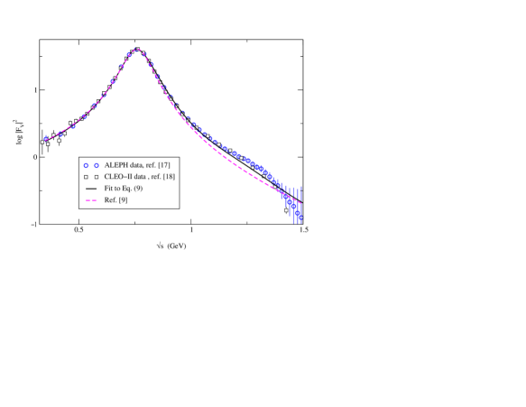
Figure 1: Comparison of the result of the fit to ALEPH data with the experimental ALEPH [17] and CLEO-II [18] data on $F_{V}(s)$ from $\tau^{-}\rightarrow\pi^{-}\pi^{0}\nu_{\tau}$ in the $\rho(770)$ energy region. The result of Ref. [9] for $M_{\rho}=775\,\mbox{MeV}$ is also shown. Up to $\sqrt{s}\sim 0.8\,\mbox{GeV}$ both curves are almost indistinguishable.

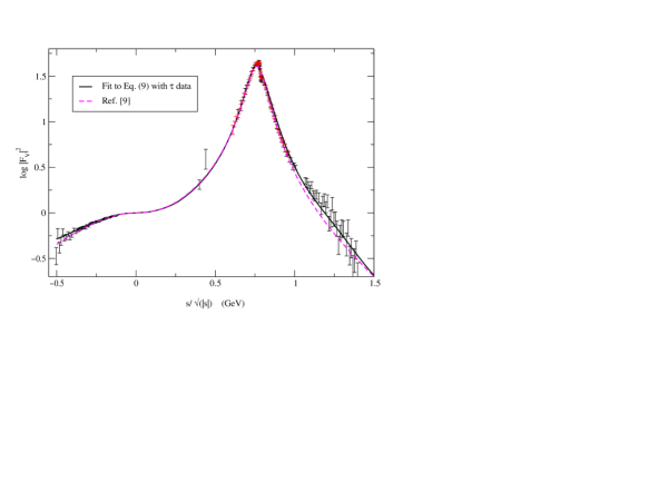
Figure 2: Comparison of the result of our fit with the experimental data on $F_{V}(s)$ from $e^{+}e^{-}\rightarrow\pi^{+}\pi^{-}$ (time–like) [15] and $e^{-}\pi^{\pm}\rightarrow e^{-}\pi^{\pm}$ (space–like) [16]. The result of Ref. [9] ($M_{\rho}=775\,\mbox{MeV}$) is also shown. In the region $-0.4\,\mbox{GeV}\stackrel{{\scriptstyle<}}{{{}_{\sim}}}\,s/\sqrt{|s|}\,\stackrel{{\scriptstyle<}}{{{}_{\sim}}}0.8\,\mbox{GeV}$ both curves are almost indistinguishable.

In Fig. 1 we compare the experimental data with our prescription. We also include the parameter–free prediction (1 subtraction only) of Ref. [9] that, for completeness, we recall in Appendix A. It can be seen that our fit gives a good description of data up to $E\sim 1.3\,\mbox{GeV}$. Experimental data (in spite of the big errors in the higher energy region) seem to have a determinate structure (mild shoulder) around $E\sim 1.3\,\mbox{GeV}$. This could be due to a heavier $\rho$–like resonance as the $\rho(1450)$. Our solution takes into account this possibility though, because Ochs data embody these resonances up to $E\sim 1.5\,\mbox{GeV}$.

We can compare the results of our fit to tau decay data with the experimental results coming from $e^{+}e^{-}\rightarrow\pi^{+}\pi^{-}$ (time–like) [15] and $e^{-}\pi^{\pm}\rightarrow e^{-}\pi^{\pm}$ (space–like) [16] processes. In Fig. 2 we show these sets of data together with the same curves of Fig. 1. We conclude that the agreement of our fit with data is good within the errors. Notice that $e^{+}e^{-}\rightarrow\pi^{+}\pi^{-}$ data has a contribution from $\omega(782)$ that translates into a slight deformation on the right–hand side of the $\rho(770)$ peak. This is due to a small $I=0$ component contributing to the $2\pi$ spectral function in $e^{+}e^{-}\rightarrow\pi^{+}\pi^{-}$. This contribution does not appear in the isovector spectral function from $\tau^{-}\rightarrow\pi^{-}\pi^{0}\nu_{\tau}$ which we are describing.

4 The low–energy observables

At $E<2m_{\pi}$ the vector pion form factor satisfies a low–energy expansion given by Eq. (10). Up to the quadratic term in $s$ we have, therefore, two low–energy observables, the squared charge radius of the pion, $\langle r^{2}\rangle^{\pi}_{V}$, and the quadratic term $c^{\pi}_{V}$, that are related with the parameters $\alpha_{1}$ and $\alpha_{2}$ of the form factor (9) as given in Eq. (11).

$\langle r^{2}\rangle^{\pi}_{V}$ and $c^{\pi}_{V}$ have recently been determined at ${\cal O}(p^{6})$ in $\chi$PT [8]. While chiral symmetry constraints successfully provide the chiral logarithms, it remains an incertitude in the polynomial part that involves counterterms not predicted by the chiral framework. Therefore it is not possible to give a plain prediction for these observables. The authors of Ref. [8] performed, by including properly the chiral logarithms, a fit of the pion form factor, as given by ${\cal O}(p^{6})$ $\chi$PT, to the data from $\tau^{-}\rightarrow\pi^{-}\pi^{0}\nu_{\tau}$, $e^{+}e^{-}\rightarrow\pi^{+}\pi^{-}$ and $e^{-}\pi^{\pm}\rightarrow e^{-}\pi^{\pm}$ in the low–energy region ($E\stackrel{{\scriptstyle<}}{{{}_{\sim}}}0.5\,\mbox{GeV}$). Our procedure provides the low–energy observables from a fit to a larger energy interval in the time–like region. In Table 1 we compare our figures with those of Ref. [8]. As can be seen the results compare very well but the errors to the observables provided by our procedure are smaller (noticeably in $c_{V}^{\pi}$).

	$\langle r^{2}\rangle^{\pi}_{V}\,(\mbox{GeV}^{-2})$	$c^{\pi}_{V}\,(\mbox{GeV}^{-4})$
Our fit	$11.04\pm 0.30$	$3.79\pm 0.04$
${\cal O}(p^{6})$ $\chi$PT	$11.22\pm 0.41$	$3.85\pm 0.60$

Table 1: Low–energy observables of the vector pion form factor up to the quadratic term. We give the results for our fit and the ${\cal O}(p^{6})$ $\chi$PT analysis of Ref.[8].

	$r^{V}_{V_{1}}(M_{\rho})\times 10^{3}$	$r^{V}_{V_{2}}(M_{\rho})\times 10^{4}$
Our fit	$-0.79\pm 0.19$	$1.46\pm 0.03$
${\cal O}(p^{6})$ $\chi$PT	$-0.68\pm 0.26$	$1.50\pm 0.44$
VMD	$-0.25$	$2.6$

Table 2: Combination of ${\cal O}(p^{6})$ counterterms appearing in the $\chi$PT evaluation of $\langle r^{2}\rangle^{\pi}_{V}$ and $c^{\pi}_{V}$. We give the predictions from our fit and the ones from the chiral fit and the VMD result of Ref.[8].

As commented above the predictability of $\chi$PT at ${\cal O}(p^{6})$ is spoiled because chiral symmetry does not provide information on the finite part of the counterterms in the results of $\langle r^{2}\rangle^{\pi}_{V}$ and $c^{\pi}_{V}$. Two combinations of ${\cal O}(p^{6})$ counterterms, $r^{r}_{V_{1}}(M_{\rho})$ and $r^{r}_{V_{2}}(M_{\rho})$, one on each observable, have to be considered. In order to predict these terms one has to rely in modelizations or dynamical assumptions like Vector Meson Dominance (VMD). This last resource was employed in Ref. [8] to evaluate the vector resonance contributions $r_{V_{1}}^{V}(M_{\rho})$, $r_{V_{2}}^{V}(M_{\rho})$ that is the dominant piece by far.

Numerically the ${\cal O}(p^{6})$ $\chi$PT expressions relating the low–energy observables with the polynomial terms are

$$\langle r^{2}\rangle^{\pi}_{V}\, = \,\left[\,12.312\,+\,1603.4\,r^{V}_{V_{1}}(M_{\rho})\,\right]\,(\mbox{GeV}^{-2})\;\;,$$

$$c^{\pi}_{V}\, = \,\left[\,1.787\,+\,13718.7\,r^{V}_{V_{2}}(M_{\rho})\,\right]\,(\mbox{GeV}^{-4})\;\;.$$ (14)

Within VMD these counterterms are obtained by integrating out vector resonances using the resonance chiral theory framework [6]. They have been worked out, within the Proca formalism, in Ref. [8] with the results

$$r_{V_{1}}^{V}\, = \,2\sqrt{2}\frac{\displaystyle F_{\pi}^{2}}{\displaystyle M_{V}^{2}}\,f_{\chi}f_{V}\;\;,$$

$$r_{V_{2}}^{V}\, = \,\frac{\displaystyle F_{\pi}^{2}}{\displaystyle M_{V}^{2}}\,g_{V}f_{V}\;\;,$$ (15)

obtained by integrating the lightest octet of vector resonances of mass $M_{V}$. The couplings $f_{V}$, $g_{V}$ and $f_{\chi}$ can be phenomenologically obtained from $\rho\rightarrow e^{+}e^{-}$, $\rho\rightarrow\pi^{+}\pi^{-}$ and $\phi\rightarrow K\overline{K}$ with the results: $f_{V}=0.20$, $g_{V}=0.09$ and $f_{\chi}=-0.03$, and, therefore, giving values for $r_{V_{i}}^{V}$ that we collect in Table 2. We compare these VMD results with the ones obtained from our fit and the ones provided by the ${\cal O}(p^{6})$ $\chi$PT fit. We notice that the result of VMD seems to undervalue $|r^{V}_{V_{1}}(M_{\rho})|$ and overestimates $r^{V}_{V_{2}}(M_{\rho})$. As can be seen from Eq. (14) this difference would affect most the value of $c^{\pi}_{V}$. It has to be observed though that, on one side, to extract $r^{V}_{V_{1}}(M_{\rho})$ from $\langle r^{2}\rangle^{\pi}_{V}$ in Eq. (14) a strong cancellation driven by the term $(\langle r^{2}\rangle^{\pi}_{V}-12.312)$ is involved and therefore it is very sensitive to the value of the squared charge radius of the pion (this problem does not arise in the $r^{V}_{V_{2}}(M_{\rho})$ case); on the other side, VMD can only offer a rough estimate because, at this order, heavier resonances could also give a noticeable contribution while the VMD result only includes the lightest octet of vector mesons. By neglecting these heavier states we could invert the procedure and use our fit to predict the products of couplings $f_{\chi}f_{V}$ and $g_{V}f_{V}$ from Eq. (15). We obtain, for example, $f_{\chi}/g_{V}=(-1.9\pm 0.6)$ far from the phenomenological value $f_{\chi}/g_{V}\simeq-0.33$. It looks as if the role of heavier resonances is crucial in order to describe ${\cal O}(p^{6})$ vector driven contributions in $\chi$PT.

5 Two–pion contribution to the muon $(g-2)$ and to $\alpha(M_{Z}^{2})$

The hadronic contribution to the anomalous magnetic moment $a_{\mu}=(g_{\mu}-2)/2$ of the muon is the main source of incertitude in its theoretical prediction. Its leading part comes from the photon vacuum polarization insertion into the electromagnetic vertex of the muon. It gives [22] :

$$a_{\mu}^{had}(vac.\,pol.)\,=\,(692.4\pm 6.2)\times 10^{-10}\;\;.$$ (16)

This contribution can be evaluated in terms of the experimental hadronic total cross–section $\sigma(e^{+}e^{-}\rightarrow\mbox{hadrons})$, where $e^{+}e^{-}\rightarrow\pi^{+}\pi^{-}$ is, by far, the dominant part at low energies. The bulk, both of the central value ($\sim 75\%$) and the error ($\sim 80\%$), of $a_{\mu}^{{had}}$ in Eq. (16) comes from this $\pi\pi$ intermediate state [23].

The relevant dispersion integral to evaluate this contribution is (up to two loops) [24]

$$a_{\mu}^{\pi\pi}\; = \;\left(\frac{\displaystyle\alpha(0)\,m_{\mu}}{\displaystyle 3\,\pi}\right)^{2}\,\int_{4m_{\pi}^{2}}^{\infty}\,\frac{\displaystyle ds}{\displaystyle s^{2}}\,R_{\pi\pi}(s)\,\hat{K}(s)\;\;\;,$$

$$R_{\pi\pi}(s)\; = \;\frac{\displaystyle 3\,s}{\displaystyle 4\,\pi\,\alpha^{2}(s)}\,\sigma(e^{+}e^{-}\rightarrow\pi^{+}\pi^{-})\;\;,$$

where the $\hat{K}(s)$ function is given in Ref. [25]. In terms of $F_{V}(s)$ we have

$$a_{\mu}^{\pi\pi}\;=\;\left(\frac{\displaystyle\alpha(0)\,m_{\mu}}{\displaystyle 6\,\pi}\right)^{2}\,\int_{4m_{\pi}^{2}}^{\Lambda^{2}}\,\frac{\displaystyle ds}{\displaystyle s^{2}}\,\sigma_{\pi}^{3}\,|F_{V}(s)|^{2}\,\hat{K}(s)\;\;,$$ (18)

where we have introduced a cut–off $\Lambda$ as the upper limit of integration. As $\hat{K}(s)$ grows mildly at high values of $s$, the integration in $a_{\mu}^{\pi\pi}$ in Eq. (18) is dominated by the very low–energy region that gives the main contribution.

The hadronic contribution to the shift in the fine structure constant $\Delta\alpha(s)$, defined through $\alpha(s)=\alpha(0)/(1-\Delta\alpha(s))$, can be evaluated from $e^{+}e^{-}\rightarrow\mbox{\em hadrons}$ data by using a dispersion relation together with the optical theorem [26]. The last estimation has been worked out in Ref. [22] giving

$$\Delta\alpha^{(5)}(M_{Z}^{2})|_{had}\,=\,(276.3\pm 1.6)\times 10^{-4}\;\;,$$ (19)

where the superscript indicates that only the 5 lightest quark flavours have been considered.

The $\pi\pi$ contribution can be accounted for by

$$\Delta\alpha(M_{Z}^{2})|_{\pi\pi}\;=\;-\,\frac{\displaystyle\alpha(0)\,M_{Z}^{2}}{\displaystyle 12\,\pi}\,\int_{4m_{\pi}^{2}}^{\Lambda^{2}}\,ds\,\frac{\displaystyle\sigma_{\pi}^{3}\,|F_{V}(s)|^{2}}{\displaystyle s(s-M_{Z}^{2})}\;\;,$$ (20)

where, once more, we have introduced a cut–off $\Lambda$ as the upper limit of integration in order to control the good description of the integrand. Contrarily to what happens in the $a_{\mu}^{\pi\pi}$ case, from Eq. (20) we see that the integrand is not so dominated by the low–energy region and, therefore, higher energy contributions are relevant to evaluate $\Delta\alpha(M_{Z}^{2})|_{\pi\pi}$. In addition, and as we will see, the $\pi\pi$ contribution to $\Delta\alpha(M_{Z}^{2})|_{had}$ in this energy region is just a modest $10\%$ of the full value (19).

$\Lambda$ (GeV)	$a_{\mu}^{\pi\pi}\times 10^{10}$	$\Delta\alpha(M_{Z}^{2})|_{\pi\pi}\times 10^{4}$
1.0	$505\pm 6$	$33.8\pm 0.4$
1.1	$511\pm 6$	$34.7\pm 0.5$
1.2	$514\pm 6$	$35.1\pm 0.5$
1.3	$516\pm 6$	$35.4\pm 0.5$

Table 3: Values of $a_{\mu}^{\pi\pi}$ and $\Delta\alpha(M_{Z}^{2})|_{\pi\pi}$ given by our fit to ALEPH $\tau$ decay data, in the whole energy range ($0.32\,\mbox{GeV}\leq\sqrt{s}\leq 1.6\,\mbox{GeV}$), for different values of the $\Lambda$ cut–off.

The study on the vector form factor of the pion that we have carried out allows us to put forward a prediction for both $a_{\mu}^{\pi\pi}$ and $\Delta\alpha(M_{Z}^{2})|_{\pi\pi}$ that we work out as follows. The fit to ALEPH data that gave our results in Eq. (13) was limited to $\sqrt{s}\leq 1.1\,\mbox{GeV}$. As commented there we took this region because we have a thorough control of the physics involved within. At higher energies new physics input, unaccounted for, appears. As a result, in Fig. 1 it can be seen that our fit misses barely the data above $\sqrt{s}\sim 1.2\,\mbox{GeV}$, well outside the fitted region. The computation of the integrals in $a_{\mu}^{\pi\pi}$ (18) and $\Delta\alpha(M_{Z}^{2})|_{\pi\pi}$ (20) requires a good knowledge of $F_{V}(s)$ up to $s\simeq\Lambda^{2}$, therefore if we wish to reach $\Lambda\simeq 1.3\,\mbox{GeV}$ we would need a better description of data than the one given with the parameters in Eq. (13). To achieve this feature we fix $M_{\rho}=775.1\,\mbox{MeV}$, as concluded in Eq. (13), and leave $\alpha_{1}$, $\alpha_{2}$ as free parameters. Then we fit the ALEPH data in the whole range $0.32\,\mbox{GeV}\leq\sqrt{s}\leq 1.6\,\mbox{GeV}$. By studying, as above, the stability of the fitted parameters against variations in the number of subtractions, the upper limit $\Lambda$, and the matching point $\sqrt{s_{match}}$, we conclude the values $\widetilde{\alpha_{1}}=(1.83\pm 0.03)\,\mbox{GeV}^{-2}$, $\widetilde{\alpha_{2}}=(4.28\pm 0.08)\,\mbox{GeV}^{-4}$, consistent with the solution of the restricted fit (13) but with smaller errors. The tildes on $\alpha_{1}$ and $\alpha_{2}$ are meant to prevent their use in Eq. (11). We emphasize that $\widetilde{\alpha_{1}}$ and $\widetilde{\alpha_{2}}$ are not proper physical values of the $\alpha_{1}$, $\alpha_{2}$ parameters because we have fitted a region of experimental data that is not properly implemented theoretically. However the above values of $\widetilde{\alpha_{1}}$ and $\widetilde{\alpha_{2}}$ describe well data up to $\sqrt{s}\simeq 1.3\,\mbox{GeV}$ and, therefore, are useful to evaluate the integrals in $a_{\mu}^{\pi\pi}$ and $\Delta\alpha(M_{Z}^{2})|_{\pi\pi}$ with smaller errors. The values we get are collected in Table 3.

It has to be noticed that our errors are similar to those obtained in recent estimations [23], though the results in this reference were obtained from a combination of $e^{+}e^{-}\rightarrow\pi\pi$ and $\tau^{-}\rightarrow\pi^{-}\pi^{0}\nu_{\tau}$ decay data while our results come from a fit to this last process up to $\sqrt{s}\simeq 1.6\,\mbox{GeV}$. An improvement on our errors would require an analysis of the pion vector form factor with a more complete set of data, combining $e^{+}e^{-}\rightarrow\pi\pi$ and $\tau^{-}\rightarrow\pi^{-}\pi^{0}\nu_{\tau}$ processes.

6 Conclusions

To gain access to the resonance properties, from experimental data, a correct definition of those properties has to be theoretically implemented. The use of modelizations, though sometimes unavoidable, can spoil seriously the conclusions obtained from data. In this article we have studied the vector pion form factor $F_{V}(s)$ within a model–independent approach. We have introduced a parameterization of the form factor provided by the all–important properties of its analyticity and unitarity relations. This last construction relates $F_{V}(s)$ to the $\delta_{1}^{1}(s)$ phase–shift of elastic $\pi\pi$ scattering.

To proceed we have included the $\delta_{1}^{1}(s)$ phase–shift (up to $\sqrt{s}\simeq 1.5\,\mbox{GeV}$) with a model–independent parameterization, provided by the resonance chiral theory and experimental data. Our form factor depends on two, a priori unknown, subtraction constants and the $\rho(770)$ mass. We have fitted ALEPH data on $\tau^{-}\rightarrow\pi^{-}\pi^{0}\nu_{\tau}$ to the form factor for $E\stackrel{{\scriptstyle<}}{{{}_{\sim}}}1.1\,\mbox{GeV}$ and we obtain $M_{\rho}=(775.1\pm 0.5)\,\mbox{MeV}$. Our result for $M_{\rho}$ is bigger than the new average of the Review of Particle Properties [13] but very much consistent with their average from $\tau$ decays and $e^{+}e^{-}$ annihilation processes. The predictions given by our results on the low–energy observables worked out in $\chi$PT, $\langle r^{2}\rangle_{V}^{\pi}$ and $c_{V}^{\pi}$ have also been computed. We find good agreement with the results from the fit in $\chi$PT though our errors are smaller. It is necessary to notice, though, that when these figures are worked on to determine local chiral ${\cal O}(p^{6})$ counterterms, the values we get are not consistent with those obtained, through VMD, from resonance chiral theory by integrating out the lightest octet of vector resonances. As a conclusion it seems that room is left for the contribution of heavier resonances.

Finally we have evaluated the $\pi\pi$ contribution to the anomalous magnetic moment of the muon, $a_{\mu}^{\pi\pi}$, and the shift of the fine structure constant $\Delta\alpha(M_{Z}^{2})|_{\pi\pi}$. An improvement in the theoretical errors of these quantities would be achieved with a more complete analysis of the available data.

We have shown how it is possible to extract model–independent information of resonances from experimental data by exploiting general properties of form factors, such as unitarity and analyticity. When combined with the resonance chiral theory, the effective action of QCD at the lightest resonance region, these properties provide a compelling framework for the study of form factors.
Acknowledgements

      We wish to thank Jon Urheim for correspondence on the $\tau$ decay data from CLEO-II. This work has been supported in part by TMR, EC–Contract No. ERB FMRX-CT98-0169 and by CICYT (Spain) under grant PB97-1261.

Appendix A

A theoretical construction of the vector form factor of the pion was performed in Ref. [9] by matching the ${\cal O}(p^{4})$ $\chi$PT result (valid at $E\ll M_{\rho}$) with the prescription provided by the resonance chiral theory. The procedure also took into account the analyticity and unitarity properties of $F_{V}(s)$. The result only includes the contribution of the $\rho(770)$ resonance and gives an excellent description of data up to $E\sim 1\,\mbox{GeV}$ with just one parameter, $M_{\rho}$. We have compared this prescription with ours in Figures 1 and 2.

For completeness we recall here the result of Ref. [9]:

$$F_{V}(s)\,=\,\frac{\displaystyle M_{\rho}^{2}}{\displaystyle M_{\rho}^{2}\,-\,s\,-\,iM_{\rho}\Gamma_{\rho}(s)}\, \!\!\!\!\!\!\!\!\exp\left\{\,\frac{\displaystyle-s}{\displaystyle 96\pi^{2}F_{\pi}^{2}}\,\left[\,\mbox{Re}A\left(m_{\pi}^{2}/s,m_{\pi}^{2}/M_{\rho}^{2}\right)\,+\right.\right.$$ (A.1)

$$\left.\left.\;\;\;\;\;\;\;\;\;\;\;\;\;\;\;\;\;\;\,\frac{\displaystyle 1}{\displaystyle 2}\,\mbox{Re}A\left(m_{K}^{2}/s,m_{K}^{2}/M_{\rho}^{2}\right)\,\right]\right\}\;,$$

where $\Gamma_{\rho}(s)$ is the hadronic off–shell width of the $\rho(770)$ resonance [12],

$$\Gamma_{\rho}(s)\,=\,\frac{\displaystyle M_{\rho}s}{\displaystyle 96\pi F_{\pi}^{2}}\,\left[\sigma_{\pi}^{3}\theta(s-4m_{\pi}^{2})\,+\,\frac{1}{2}\sigma_{K}^{3}\theta(s-4m_{K}^{2})\,\right]\;\;,$$ (A.2)

and

$$A\left(m_{P}^{2}/s,m_{P}^{2}/\mu^{2}\right)\,=\,\ln\left(\frac{\displaystyle m_{P}^{2}}{\displaystyle\mu^{2}}\right)\,+\,8\,\frac{\displaystyle m_{P}^{2}}{\displaystyle s}\,-\,\frac{\displaystyle 5}{\displaystyle 3}\,+\,\sigma_{P}^{3}\,\ln\left(\frac{\displaystyle\sigma_{P}+1}{\displaystyle\sigma_{P}-1}\right)\;\;,$$ (A.3)

with $\sigma_{P}=\sqrt{1-4m_{P}^{2}/s}$.

References

- [1] G.J. Gounaris and J.J. Sakurai, Phys. Rev. Lett. 21, 244 (1968).
-
[2]
A. Pich, “QCD Tests from Tau Decay Data”, Proc.
“Tau-Charm Factory Workshop”,
(SLAC, Stanford, 1989), ed. L. V. Beers,
SLAC-Report-343 (1989) p. 416;
J.H. Kühn and A. Santamaria, Z. Phys. C48, 445 (1990). -
[3]
S. Jadach and Z. Was, Comput. Phys. Commun. 36, 191
(1985);
S. Jadach, J.H. Kühn and Z. Was, Comput. Phys. Commun, 76, 361 (1993). -
[4]
S. Weinberg, Physica 96A, 327 (1979) ;
J. Gasser and H. Leutwyler, Ann. of Phys. (NY) 158, 142 (1984);
J. Gasser and H. Leutwyler, Nucl. Phys. B250, 465 (1985). -
[5]
G. Ecker, Prog. Part. Nucl. Phys. 35, 1 (1995) ;
U. G. Meissner, Rept. Prog. Phys. 56, 903 (1993);
A. Pich, Rep. Prog. Phys. 58, 563 (1995). -
[6]
G. Ecker, J. Gasser, A. Pich and E. de Rafael,
Nucl. Phys. B321, 311 (1989) ;
G. Ecker, J. Gasser, H. Leutwyler, A. Pich and E. de Rafael, Phys. Lett. B223, 425 (1989). - [7] J. Gasser and H. Leutwyler, Nucl. Phys. B250, 517 (1985).
- [8] J. Bijnens, G. Colangelo and P. Talavera, J. High Energy Phys. 05, 014 (1998).
- [9] F. Guerrero and A. Pich, Phys. Lett. B412, 382 (1997).
- [10] K.M. Watson, Phys. Rev. 88, 1163 (1952).
-
[11]
N.I. Muskhelishvili, Singular Integral Equations,
(Noordhoof, Groningen, 1953);
R. Omnès, Nuovo Cimento 8, 316 (1958). - [12] D. Gómez Dumm, A. Pich and J. Portolés, Phys. Rev. D62, 054014 (2000).
- [13] D.E. Groom et al, Review of Particle Properties, Eur. Phys. J. C15, 1 (2000); http://pdg.lbl.gov.
- [14] W. Ochs, Univ. of Munich thesis (1973).
- [15] Barkov et al., Nucl. Phys. B256, 365 (1985).
- [16] Amendolia et al., Nucl. Phys. B277, 168 (1986).
- [17] R. Barate et al., ALEPH Col., Z. Phys. C76, 15 (1997).
- [18] S. Anderson et al., CLEO-II Col., Phys. Rev. D61, 112002 (2000).
- [19] K. Ackerstaff et al., OPAL Col., Eur. Phys. J. C7, 571 (1999).
- [20] J.A. Oller, E. Oset and J.E. Palomar, hep–ph/0011096.
- [21] F. James and M. Roos, Comput. Phys. Commun. 10, 343 (1975).
-
[22]
M. Davier and A. Höcker, Phys. Lett. B435, 427 (1998);
M. Davier, talk given at the Sixth International Workshop on Tau Lepton Physics, Victoria (Canada), September 2000. To appear in the proceedings. - [23] R. Alemany, M. Davier and A. Höcker, Eur. Phys. J. C2, 123 (1998).
- [24] M. Gourdin and E. de Rafael, Nucl. Phys. B10, 667 (1969).
- [25] S. Eidelman and F. Jegerlehner, Z. Phys. C67, 585 (1995).
- [26] N. Cabbibo and R. Gatto, Phys. Rev. Lett. 4, 313 (1960).