KA-TP-25-2000

UAB-FT-505

hep-ph/0101086

Abstract

We present results on the full one-loop electroweak radiative corrections to the squark decay partial widths into charginos and neutralinos. We show the renormalization framework, and present numerical results for the third squark family. The corrections can reach values of $\sim 10\%$, which are comparable to the radiative corrections from the strong sector of the model. Therefore they should be taken into account for the precise extraction of the SUSY parameters at future colliders.

The Standard Model (SM) of the strong and electroweak interactions is the present paradigm of particle physics. Its validity has been tested to a level better than one per mil in the particle accelerators [1]. Nevertheless, there are arguments against the SM being the fundamental model of particle interactions [2], giving rise to the investigation of competing alternative or extended models, which can be tested at high-energy colliders, such as the Large Hadron Collider (LHC) [3], or a $e^{+}e^{-}$ Linear Collider (LC) [4]. One of the most promising possibilities for physics beyond the SM is the incorporation of Supersymmetry (SUSY), which leads to a renormalizable field theory with precisely calculable predictions to be tested in future experiments. The simplest supersymmetric extension of the SM is the Minimal Supersymmetric Standard Model (MSSM) [5]. If the masses of the extra non-standard particles are very large as compared to the SM electroweak scale, the effects of these particles decouple from the SM low-energy effective Lagrangian [6]. This means that if the extra particles are too heavy we could not discern between the SM and the MSSM by just looking at the low-energy end of the spectrum, since the only trace of the MSSM would be a light Higgs boson ($M_{h^{0}}\mbox{ \raisebox{-4.0pt}{${\stackrel{{\scriptstyle\textstyle<}}{{\sim}}}$} }135\mbox{ GeV}$) [7], whose properties would not differ from the SM one. Nevertheless, when some of the extra particle masses are of the order of the electroweak scale, the next generation of colliders will be able to produce such kind of particles and investigate their properties. In this case non-decoupling effects appear [8, 9]. While the LHC will be able to produce new particles with masses up to $2.5\mbox{ TeV}$, the LC will be able to make precision measurements of their properties, provided they are not too heavy. For an adequate analysis, precise theoretical predictions are required, going beyond the Born approximation for SUSY processes.

Up to now the major effort on the computation of SUSY radiative corrections has been put into the computation of virtual SUSY effects in observables that involve only SM external particles, or into the calculation of loop effects in the extended Higgs sector of the MSSM. But for the case of direct production of SUSY particles, one also needs a detailed knowledge of the higher-order effects for the processes with these SUSY particles in the external states. A number of studies have already addressed this issue, for production as well as for decay processes. For squark and gluino production in hadron collisions, the NLO QCD corrections are available [11]; for squark-pair production in $e^{+}e^{-}$ collisions, the NLO QCD are also known, together with the Yukawa corrections [12]. Concerning the subsequent squark decays into charginos/neutralinos, the QCD corrections were presented in [13, 8], whereas the Yukawa corrections were given in [15]. In this last work large corrections were found. They were derived, however, in the higgsino approximation for the chargino; hence, a full computation is required to consolidate the significance of the loop effects.

In this letter we present, for the first time, a complete one-loop computation of the electroweak radiative corrections to the partial decay widths of squarks into quarks and charginos/neutralinos,

$$\Gamma(\tilde{q}\to q^{\prime}\chi)\,\,,$$ (1)

with $\tilde{q}=\tilde{b},\,\tilde{t}$, $q=b,\,t$, $\chi=\chi^{0}_{\alpha},\,\chi^{\pm}_{i}$. We present the basic structure of the corrections, and illustrate their main features and their significance in representative numerical examples. The fine details, as well as a comprehensive analysis, will be presented elsewhere [9]. Although the explicit results, for definiteness, are displayed for the third squark generation, our analytic results are valid for all kinds of squarks.

In processes with exclusively SM particles in external states, it is possible to divide the 1-loop contributions into SM-like and non-SM-like subclasses. This separate treatment is often used in the literature, and it is useful since it allows to make the computation in small steps, checking each sector individually. As a distinctive feature of the radiative corrections to processes with supersymmetric particles in the external legs, this separability is lost. In this kind of processes the ultraviolet (UV) divergences of diagrams with virtual SM particles cancel the UV divergences of diagrams with non-SM particles. Any partial computation would yield UV-divergent and thus meaningless results. For this reason we have to compute all the SM and non-SM loop contributions at once, with the proper counter terms involving the renormalization of almost the full MSSM.

We have used an on-shell renormalization scheme, which can be obtained by extending the on-shell scheme of [16] to the MSSM. For the SM sector, the gauge-boson and fermion masses are treated as input parameters; the electron charge is defined in the Thomson limit, and the weak mixing angle is given in terms of $\sin\theta_{W}^{2}\equiv s_{W}^{2}\equiv 1-M^{2}_{W}/M^{2}_{Z}$. The SM sector and its renormalization is described in [16] and will not be repeated here. On the other hand, different conventions for the SUSY sector exist; therefore, a few comments on our procedure are in order. Concerning the Higgs sector, one mass has to be specified as an input quantity (for which we take the mass of the $H^{\pm}$), and a definition for $\tan\beta$, the ratio between the vacuum expectation value of the two Higgs-boson doublets, $v_{2}/v_{1}$, is needed. Following [17], an indirect definition of $\tan\beta$ is given by the requirement $\delta v_{2}/v_{2}={\delta v_{1}}/{v_{1}}$. For the sfermion sector, we use the input and the renormalization conditions as described in [15], which fixes the squark masses and the squark-mixing angles $\theta_{\tilde{q}}$.

Finally, as a new ingredient, we have to specify the chargino–neutralino sector. The tree-level mass matrices are well known, but we list them in order to settle the conventions:

$${\cal M} = \pmatrix{M&\sqrt{2}M_{W}\sin{\beta}\cr\sqrt{2}M_{W}\cos{\beta}&\mu}\,\,,$$

$${\cal M}^{0} = \pmatrix{M^{\prime}&0&M_{Z}\cos{\beta}s_{W}&-M_{Z}\sin{\beta}s_{W}\cr 0&M&-M_{Z}\cos{\beta}c_{W}&M_{Z}\sin{\beta}c_{W}\cr M_{Z}\cos{\beta}s_{W}&-M_{Z}\cos{\beta}c_{W}&0&-\mu\cr-M_{Z}\sin{\beta}s_{W}&M_{Z}\sin{\beta}c_{W}&-\mu&0}\,\,\,.$$ (2)

$M$ and $M^{\prime}$ are the $SU(2)_{L}$ and $U(1)_{Y}$ soft-SUSY-breaking gaugino masses. These mass matrices are diagonalized by unitary matrices $U,V,N$ via

$$\begin{array}[]{lcccl}U^{*}{\cal M}V^{\dagger}&=&{\cal M}_{D}&=&{\rm diag}\left(M_{1},M_{2}\right)\,\,(0<M_{1}<M_{2})\,\,,\\ N^{*}{\cal M}^{0}N^{\dagger}&=&{\cal M}^{0}_{D}&=&{\rm diag}\left(M_{1}^{0},M_{2}^{0},M_{3}^{0},M_{4}^{0}\right)\,\,(0<M_{1}^{0}<M_{2}^{0}<M_{3}^{0}<M_{4}^{0})\,\,.\end{array}$$ (3)

This sector contains six particle masses, but only three free parameters are available for an independent renormalization. As a consequence, we are not allowed to impose on-shell conditions for all the particle masses. For the independent input parameters, we choose: the masses of the two charginos and the mass of the lightest neutralino. By introducing counterterms for all the independent parameters in (2), we are able to relate the counterterms of the fundamental parameters to the mass-counterterms $\delta M_{i}$ of the charginos. Similarly to [19] we find:

$$M_{1}\,\delta M_{1}+M_{2}\,\delta M_{2} = M\,\delta M+\mu\,\delta\mu+\delta M^{2}_{W},$$

$$M_{1}M_{2}\left(M_{1}\,\delta M_{2}+M_{2}\,\delta M_{1}\right) = \left(M\mu-M^{2}_{W}\sin(2\beta)\right)\bigg{[}M\,\delta\mu+\mu\,\delta M$$ (4)

$$-M^{2}_{W}\,\delta\sin(2\beta)-\sin(2\beta)\,\delta M^{2}_{W}\bigg{]}.$$

The mass counterterms $\delta M_{i}$ are fixed using the on-shell scheme relation, in the convention of [16] (but with opposite sign for $\Sigma$),

$$\delta M_{i}=-\frac{1}{2}\left(\Sigma_{L}^{i}(M_{i}^{2})+\Sigma_{R}^{i}(M_{i}^{2})\right)-\Sigma_{S}^{i}(M_{i}^{2})\,\,,$$ (5)

where $\Sigma_{\{L,R,S\}}^{i}$ denote the one-loop unrenormalized left-, right-handed and scalar components of the self-energy for the $i$th-chargino. $\delta M^{\prime}$ is determined from the lightest neutralino mass, inverting the relation

$$N^{*}_{1\alpha}\delta{\cal M}^{0}_{\alpha\beta}N_{1\beta}^{*}=\delta M_{1}^{0}\,\,,$$ (6)

where the neutralino-mass counterterm $\delta M_{1}^{0}$ is fixed by the on-shell condition for $\chi^{0}_{1}$, in analogy to (5). It is a non-trivial check that with the counterterms determined in eqs. (4) and (6), the one-loop masses for the residual neutralinos, computed as the pole masses, are UV-finite. The one-loop on-shell neutralino masses read

$$M_{\alpha}^{0\ {\rm os}}=M_{\alpha}^{0}+N^{*}_{\alpha\beta}\delta{\cal M}^{0}_{\beta\gamma}N_{\alpha\gamma}^{*}+\frac{1}{2}\left(\Sigma_{L}^{\alpha}(M_{\alpha}^{02})+\Sigma_{L}^{\alpha}(M_{\alpha}^{02})\right)+\Sigma_{S}^{\alpha}(M_{\alpha}^{02})\,\,,$$ (7)

where now the parameters of eq. (2) and the masses and mixing matrices computed in (3) have to be regarded as renormalized quantities.

The choice of the lightest neutralino to fix the counterterm $\delta M^{\prime}$ in (6) is only efficient if it has a substantial bino component. If $M^{\prime}\gg(|\mu|,M)$ then $|N_{11}|\ll 1$, and the extraction of $\delta M^{\prime}$ from (6) would amplify the radiative corrections artificially. In this case it would be better to extract $\delta M^{\prime}$ from the $\alpha$th neutralino, such that $|N_{1\alpha}|$ is large. This is, however, not relevant for the scenarios which are discussed in this letter. Notice also that our renormalization procedure makes use of positive-definite mass eigenvalues for charginos and neutralinos, which require the introduction of some purely-imaginary non-zero elements in the $N$-matrix (3). Had we chosen a real $N$-matrix, with some negative eigenvalues, the various renormalization conditions would be plagued with the explicit sign of the corresponding eigenvalue (see e.g. [20]).

At one-loop, also mixing self-energies between the different neutralinos and charginos are generated, which we write as follows:

$$-i\hat{\Sigma}^{\alpha\beta}(k^{2})=-i\left(\hat{\Sigma}^{\alpha\beta}_{L}(k^{2})\hbox to0.0pt{/\hss}kP_{L}+\hat{\Sigma}^{\alpha\beta}_{R}(k^{2})\hbox to0.0pt{/\hss}kP_{R}+\hat{\Sigma}^{\alpha\beta}_{SL}(k^{2})P_{L}+\hat{\Sigma}^{\alpha\beta}_{SR}(k^{2})P_{R}\right)\,\,,\,\,\alpha\neq\beta\,\,,$$ (8)

with $\hat{\Sigma}$ denoting the renormalized two-point functions, and with the chirality projectors $P_{\{L,R\}}=1\mp\gamma_{5}$. For the neutralinos, the renormalized self-energies (8) are related to the unrenormalized ones according to

$$\hat{\Sigma}^{\alpha\beta}_{\{L,R\}}=\Sigma^{\alpha\beta}_{\{L,R\}}\,\,,\,\,\hat{\Sigma}_{SL}^{\alpha\beta}=\Sigma_{SL}^{\alpha\beta}{-N_{\alpha\gamma}\delta{\cal M}^{0*}_{\gamma\lambda}N_{\beta\lambda}}\,\,,\,\,\hat{\Sigma}_{SR}^{\alpha\beta}=\Sigma_{SR}^{\alpha\beta}{-N^{*}_{\alpha\gamma}\delta{\cal M}^{0}_{\gamma\lambda}N_{\beta\lambda}^{*}}\,\,,$$ (9)

and analogous expressions hold for the charginos.

As far as vertex renormalization is concerned, the vertex counterterms are already determined by the renormalization procedure described above. In addition to the parameter renormalization, we have introduced also a field-renormalization constant for each left- and right-handed chargino and neutralino field. As an explicit example, we list the renormalized bottom-sbottom-neutralino vertex. The tree-level interaction Lagrangian reads [18]

$$\begin{array}[]{l}{\cal L}_{\chi^{0}b\tilde{b}}=+\displaystyle{\frac{g}{\sqrt{2}}}\sum_{a=1,2}\sum_{\alpha=1,\ldots,4}\tilde{b}_{a}^{*}\bar{\Psi}_{\alpha}^{0}\left(A_{+a\alpha}^{(b)}P_{L}+A_{-a\alpha}^{(b)}P_{R}\right)\,b+\mbox{\rm h.c.}\ ,\\ A_{+a\alpha}^{(b)}=R_{1a}^{(b)}\left(N_{\alpha 2}^{*}-\frac{1}{3}t_{W}N_{\alpha 1}^{*}\right)-\sqrt{2}\lambda_{b}R_{2a}^{(b)}N_{\alpha 3}^{*}\,,\ A_{-a\alpha}^{(b)}=-\sqrt{2}\lambda_{b}R_{1a}^{(b)}N_{\alpha 3}-\frac{2}{3}t_{W}R_{2a}^{(b)}N_{\alpha 1}\,\,,\end{array}$$ (10)

where the bottom-quark Yukawa coupling is $\lambda_{b}=m_{b}/(\sqrt{2}M_{W}\cos\beta)$. Introducing the one-loop counterterms analogously to [15] we obtain the following counterterm Lagrangian [15, 18]

$$\delta{\cal L}_{\chi^{0}_{\alpha}b\tilde{b}_{a}} \equiv \displaystyle{\frac{g}{\sqrt{2}}}\tilde{b}_{a}^{*}\bar{\Psi}_{\alpha}^{0}\left(\delta\Lambda_{+a\alpha}^{(b)}P_{L}+\delta\Lambda_{-a\alpha}^{(b)}P_{R}\right)\,b+\mbox{\rm h.c.}$$

$$= \frac{1}{2}\left\{\left[\frac{\delta\alpha}{\alpha}+\frac{c_{W}^{2}}{s_{W}^{2}}\left(\frac{\delta M^{2}_{W}}{M^{2}_{W}}-\frac{\delta M^{2}_{Z}}{M^{2}_{Z}}\right)\right]+\delta Z_{a}\right\}{\cal L}_{\chi^{0}_{\alpha}b\tilde{b}_{a}}+{\cal L}_{\chi^{0}_{\alpha}b\tilde{b}_{c}}\delta Z_{ca}$$

$$+\Bigg{\{}\displaystyle{\frac{g}{\sqrt{2}}}\tilde{b}_{a}^{*}\bar{\Psi}_{\alpha}^{0}\left[A_{+a\alpha}^{(b)}\frac{1}{2}\left(\delta Z_{R}^{0}{}_{\alpha}+\delta Z_{L}^{b}\right)P_{L}+A_{-a\alpha}^{(b)}\frac{1}{2}\left(\delta Z_{L}^{0}{}_{\alpha}+\delta Z_{R}^{b}\right)P_{R}\right]\,b$$

$$+\displaystyle{\frac{g}{\sqrt{2}}}\tilde{b}_{a}^{*}\bar{\Psi}_{\alpha}^{0}\left(\delta A_{+a\alpha}^{(b)}P_{L}+\delta A_{-a\alpha}^{(b)}P_{R}\right)\,b+\mbox{ h.c.}\Bigg{\}}\,\,,\,\,(c\neq a)\,\,,$$

$$\delta A_{+a\alpha}^{(b)} = -\sqrt{2}\left(\delta R^{(b)}_{2a}\lambda_{b}N_{\alpha 3}+\delta\lambda_{b}R^{(b)}_{2a}N_{\alpha 3}\right)+\delta R^{(b)}_{1a}\left(N_{\alpha 2}-\frac{1}{3}t_{W}N_{\alpha 1}\right)-\frac{1}{3}\delta t_{W}R^{(b)}_{1a}N_{\alpha 1}\,\,,$$

$$\delta A_{-a\alpha}^{(b)} = -\sqrt{2}\left(\delta R^{(b)}_{1a}\lambda_{b}N^{*}_{\alpha 3}+\delta\lambda_{b}R^{(b)}_{1a}N^{*}_{\alpha 3}\right)-\frac{2}{3}t_{W}N^{*}_{\alpha 1}\left(\frac{\delta t_{W}}{t_{W}}R^{(b)}_{2a}+\delta R^{(b)}_{2a}\right)\,\,,$$

$$\frac{\delta\lambda_{b}}{\lambda_{b}} = \frac{\delta m_{b}}{m_{b}}-\frac{1}{2}\frac{\delta M^{2}_{W}}{M^{2}_{W}}-\frac{\delta\cos\beta}{\cos\beta}\,\,,\,\,\delta{t_{W}}=\frac{1}{c_{W}^{2}}\left(\frac{\delta M_{Z}^{2}}{M_{Z}^{2}}-\frac{\delta M_{W}^{2}}{M_{W}^{2}}\right),$$ (11)

where $\delta\alpha$, $\delta M_{W,Z}^{2}$ are the charge and mass counterterms for the MSSM, as given in [21]. The renormalized one-loop part of the amplitude for the decay $\tilde{b}_{a}\rightarrow b\chi^{0}_{\alpha}$ can then be written as

$$-iT_{a\alpha}^{\rm loop}=-i\frac{g}{\sqrt{2}}\bar{u}_{b}\left[C_{+\alpha\beta}P_{R}+C_{-\alpha\beta}P_{L}\right]v_{\chi^{0}_{\alpha}}\,\,;\,\,C_{\pm\alpha\beta}=\delta\Lambda_{\pm a\alpha}^{(b)*}+\Lambda_{\pm a\alpha}^{(b)}{}^{\Sigma}+\Lambda_{\pm a\alpha}^{(b)}{}^{\rm 1PI}\,\,.$$ (12)

Besides the counterterms $\delta\Lambda$ from eq. (11), it contains the one-loop contribution $\Lambda^{\rm 1PI}$ to the one-particle-irreducible three-point vertex function and the quantity $\Lambda^{\Sigma}$ representing the contribution of the neutralino-mixing self-energies (8),

$$\Lambda_{\pm a\alpha}^{(b)}{}^{\Sigma}=\sum_{\beta}A_{\pm a\beta}^{(b)*}\frac{M_{\alpha}^{0}\hat{\Sigma}_{SL}^{\beta\alpha}+M_{\beta}^{0}\hat{\Sigma}_{SR}^{\beta\alpha}+M_{\alpha}^{0}M_{\beta}^{0}\hat{\Sigma}_{L}^{\beta\alpha}+M_{\beta}^{0}{}^{2}\hat{\Sigma}_{R}^{\beta\alpha}}{M_{\alpha}^{0}{}^{2}-M_{\beta}^{0}{}^{2}}\,\,.$$ (13)

Due to the presence of photon loops, the amplitude (12) is infra-red divergent; hence, bremsstrahlung of real photons has to be added to cancel this divergence. We therefore include in our results the radiative partial decay width $\Gamma(\tilde{b}_{a}\to b\chi^{0}_{\alpha}\gamma)$, including both the soft and the hard photon part. So finally, the complete one-loop electroweak correction is given by

$$\begin{array}[]{rcl}\delta^{a\alpha}_{0}&=&\frac{\Gamma(\tilde{b}_{a}\to b\chi^{0}_{\alpha})}{\Gamma^{0}(\tilde{b}_{a}\to b\chi^{0}_{\alpha})}-1=\delta^{a\alpha}_{0{\rm virt}}+\frac{\Gamma(\tilde{b}_{a}\to b\chi^{0}_{\alpha}\gamma)}{\Gamma^{0}(\tilde{b}_{a}\to b\chi^{0}_{\alpha})}\,\,,\\[14.22636pt] \delta^{a\alpha}_{0{\rm virt}}&=&2{\rm Re}\left(\frac{(m_{\tilde{b}_{a}}^{2}-M_{\alpha}^{02}-m_{b}^{2})(A_{+a\alpha}^{(b)}C_{+a\alpha}^{(b)}+A_{-a\alpha}^{(b)}C_{-a\alpha}^{(b)})-2M_{\alpha}^{0}m_{b}(A_{+a\alpha}^{(b)}C_{-a\alpha}^{(b)}+A_{-a\alpha}^{(b)}C_{+a\alpha}^{(b)})}{(m_{\tilde{b}_{a}}^{2}-M_{\alpha}^{02}-m_{b}^{2})(|A_{+a\alpha}^{(b)}|^{2}+|A_{-a\alpha}^{(b)}|^{2})-4M_{\alpha}^{0}m_{b}{\rm Re}(A_{+a\alpha}^{(b)}A_{-a\alpha}^{(b)*})}\right)\,\,,\end{array}$$ (14)

for the neutralino decay channels, and by corresponding expressions $\delta^{ai}_{+}$ for the chargino channels, as well as for the top-squark decays.

The loop computation itself is rather tedious, since there is a huge number of diagrams to compute. This is better done by means of automatized tools. The computation of the loop diagrams has been done by using the Computer Algebra Systems FeynArts and FormCalc [22, 23]. We have produced a set of Computer Algebra programs that compute the one-loop diagrams (and the bremsstrahlung corrections), which are then plugged into a Fortran code for the numerical evaluation with the help of the one-loop routines LoopTools [23]. A number of checks has been made on the results. The UV and infra-red finiteness of the result, relying on the relations between the different sectors of the model, is a non-trivial check. We also have recovered results already available in the literature; for instance, we used our set of programs to reproduce the strong corrections of [8], and, using the higgsino approximation, we could also reproduce the results of [15]. Moreover we also checked that, when using the $\overline{\mbox{MS}}$-scheme, the one-loop corrections to neutralino and chargino masses reproduce those of [19].

Although we consider the chargino and neutralino masses as input parameters, in our numerical study we treat them in a slightly different way. We choose a set of renormalized input parameters $(M,M^{\prime},\mu)$, and apply (2), (3) to obtain the one-loop renormalized masses. Of course, if SUSY would be discovered the procedure will be the other way around, that is, the MSSM parameters will be computed from the various observables measured, for example, from the chargino production cross-section and asymmetries at the LC [24]. For a consistent treatment, the one-loop expressions for these observables will have to be used [25].

(a)
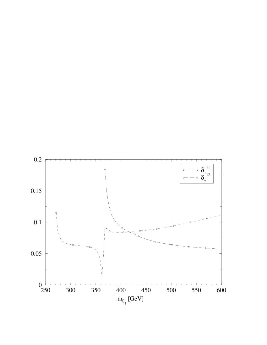
(b)	(c)

Figure 1: (a) Tree-level branching ratios for the lightest sbottom branching ratios into charginos and neutralinos as a function of the lightest sbottom mass; (b) EW radiative corrections, eq. (14), to the partial widths of lightest sbottom decaying into charginos; (c) as in (b), but for the neutralino channels.

As for the numerical analysis, we use a set of parameters relevant for the next generation of colliders. The squark masses have been chosen in the range of $\sim 300\mbox{ GeV}$. If the squarks have a mass around this scale, they will be produced at significant rates not only at the LHC, but also at a LC with $800\mbox{ GeV}$ center-of-mass energy. As for the gaugino sector, we make use of the GUT relation between the gaugino soft-SUSY-breaking mass parameters, $M^{\prime}=5/3\tan^{2}\theta_{W}M$. The input parameters for the SUSY-electroweak sector are chosen to be

$$\tan\beta=4\,\,,\,\,\mu=-100\mbox{ GeV}\,\,,\,\,M=150\mbox{ GeV}\,\,,\,\,M_{H^{\pm}}=120\mbox{ GeV}\,\,.$$ (15)

For the quark-squark sector we take

$$m_{b}=5\mbox{ GeV}\,\,,\,\,m_{\tilde{b}_{1}}=300\mbox{ GeV}\,\,,\,\,m_{\tilde{b}_{2}}=m_{\tilde{b}_{1}}+5\mbox{ GeV}\,\,,\,\,\theta_{\tilde{b}}=0.3\,\,,$$

$$m_{t}=175\mbox{ GeV}\,\,,\,\,m_{\tilde{t}_{1}}=300\mbox{ GeV}\,\,,\,\,\theta_{\tilde{t}}=0.6\,\,,$$ (16)

the rest of squarks are given a mass of $\sim 1\mbox{ TeV}$ with a mixing angle $\theta_{\tilde{q}}=\pi/4$. All over our numerical results we apply the (approximate) condition for the non-existence of colour-breaking minima, demanding that the (computed) values of the trilinear soft-SUSY-breaking couplings $A_{q}$ do not exceed $3m_{\tilde{q}}$ [26].

In Fig. 1 we present the results on the lightest-sbottom decay. Fig. 1a presents the tree-level prediction for the various branching ratios ($BR$) as a function of the lightest-sbottom mass. We see that, aside from the third neutralino channel, all the channels have an appreciable branching ratio whenever they are possible. The opening of the bosonic decay channel ($\tilde{b}_{1}\to\tilde{t}_{1}W^{-}$) is clearly visible at $m_{\tilde{b}_{1}}=m_{\tilde{t}_{1}}+M_{W}=380\mbox{ GeV}$. The charged Higgs boson channel ($\tilde{b}_{1}\to\tilde{t}_{1}H^{-}$) opens at $m_{\tilde{b}_{1}}=m_{\tilde{t}_{1}}+M_{H^{\pm}}=420\mbox{ GeV}$, but its partial width is much smaller (for the chosen value of the parameters), and hence we can not visualize its effect in Fig. 1a. Whenever the bosonic decay channels are open they amount to a large fraction of the branching ratio [27], and they suffer from large radiative corrections [28]. In Fig. 1b and c we present the one-loop electroweak radiative corrections to the chargino and neutralino channels, respectively. The lightest-neutralino channel is specially important, in that it is always open when we require the lightest neutralino to be the Lightest Supersymmetric Particle. When making a numerical scan over the MSSM parameters the corrections show a rich structure, owing to the large number of thresholds, pseudo-thresholds, etc. For example, the variation of the higgsino-mass parameter $\mu$ does not only change the chargino–neutralino masses and mixing angles, but also the value of the soft-SUSY-breaking trilinear squark couplings, and the mass of the heaviest top-squark. We see in Fig. 1a the opening of the $\tilde{b}_{1}\to t\chi^{-}_{2}$ channel at $m_{\tilde{b}_{1}}=365\mbox{ GeV}$. This threshold is accompanied by a corresponding divergence of the one-loop corrections to the lightest-chargino channel ($\delta^{11}_{+}$ in Fig. 1b), and also in the various neutralino channels (Fig. 1c). Of course, the (divergent) corrections near the threshold do not have a physical meaning, since perturbation theory breaks down. In the light-sbottom region ($m_{\tilde{b}_{1}}\mbox{ \raisebox{-4.0pt}{${\stackrel{{\scriptstyle\textstyle<}}{{\sim}}}$} }350\mbox{ GeV}$) the branching ratio is neutralino-dominated. In this region the corrections amount to a 5-10% positive corrections for all of the channels. After the opening of the $\chi^{-}_{2}$ channel the picture changes a little. The third neutralino can get corrections up to 30%, its $BR$, however, is smaller that 1%; these large corrections are thus of little interest. The rest of the channels continue with moderate corrections of the order of 5-10%; a special address to the heaviest-neutralino channel ($\chi^{0}_{4}$) with a 15% correction and a non-negligible $BR\simeq 1-8\%$ is in order. At this point, however, we do not know yet the net effect on the corrected branching ratios since the electroweak corrections are similar in all decay channels. For quantitative statements also the QCD corrections [13, 8] have to be included.

(a)
(b)	(c)

Figure 2: As in Fig. 1 but for the heaviest sbottom.

The corresponding tree-level branching ratios and radiative corrections for the heaviest bottom-squark are displayed in Fig. 2. They show a similar pattern to that of the lightest sbottom, but with more relevance for the chargino channels. We note that in this case negative radiative corrections are attained for the lightest neutralino (Fig. 2c). The maximum radiative corrections to the neutralino channel are 15% (for the heaviest neutralino), which has a non-negligible branching ratio all over the allowed sbottom-mass range. Notice that the very different corrections to the chargino channels ($\sim 17\%$ for $\chi^{-}_{1}$ and $\sim 4\%$ for $\chi^{-}_{2}$) at large sbottom masses will translate into corresponding corrections to the branching ratios.

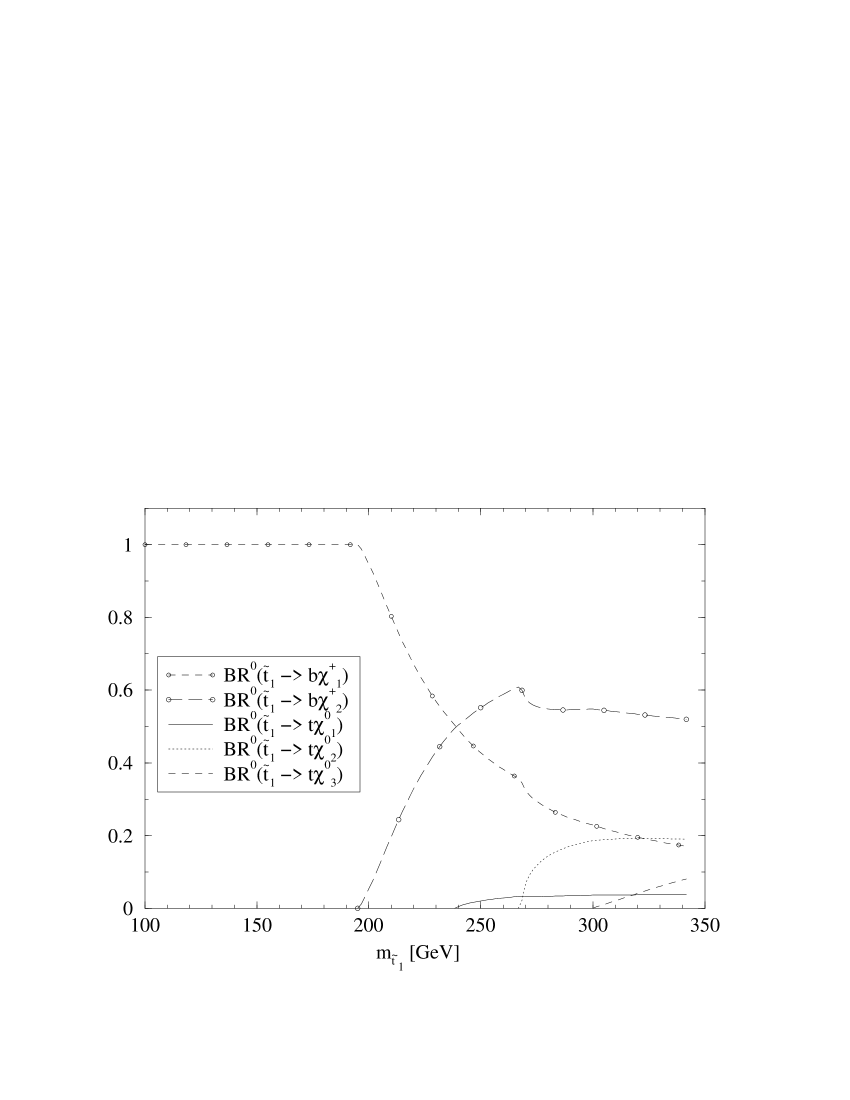
(b)	(c)

Figure 3: (a) Tree-level branching ratios for the lightest stop branching ratios into charginos and neutralinos as a function of the lightest stop mass; (b) EW radiative corrections, eq. (14), to the partial widths of lightest stop decaying into charginos and neutralinos.

We now turn our attention to the lightest-stop decay channels. In Fig. 3 we present the branching ratios and the corrections to all possible decays as a function of the lightest top-squark mass. The chargino decay channels are important whenever one of the charginos is lighter than the top-squark. The top-squark is expected to be one of the lightest squarks of the model (due to large squark mixing), it could be even lighter than the top quark. In this latter case, if the chargino channel is closed, it would decay through Flavour Changing Neutral Currents, $\tilde{t}_{1}\to c\chi^{0}_{1}$ [29]. These two decay channels have been used for a experimental simulation to extract with high precision the top-squark parameters at the LC [30]. For the chosen set of parameters the neutralino channels have never a $BR$ larger that $20\%$. When the lightest top-squark is lighter than $\sim 200\mbox{ GeV}$ the only possible decay channel has corrections to the width up to $20\%$ (Fig. 3b). These are, however, of little practical interest, since the $BR$ is 100% in any case. Above this mass, both chargino channels receive corrections in the 5-10% range. The neutralino channels obtain corrections in the 5-15% range, but, as in the case of the sbottom decays, the largest corrections occur in the channels with smallest branching ratios. Again, several threshold structures are visible in the plot, accompanied by the corresponding divergence of the corrections.

In summary, we have presented the set of full electroweak corrections to squark decays into quarks and charginos/neutralinos. These corrections can be sizeable, and therefore they have to be taken into account for the extraction of the MSSM parameters from experiment. A sample of the numerical results has been presented. The final impact on the branching ratios will also depend on the strong corrections [13, 8]. A combination of the two sets of corrections, as well as a comprehensive analysis will be presented elsewhere [9].

Acknowledgments:
The calculations have been done using the QCM cluster of the DFG Forschergruppe “Quantenfeldtheorie, Computeralgebra und Monte-Carlo Simulation”. We are thankful to T. Hahn for his help regarding the Computer Algebra system, and to A. Vicini and D. Stöckinger for useful discussions. The collaboration is part of the network “Physics at Colliders” of the European Union under contract HPRN-CT-2000-00149. The work of J.G. is supported by the European Union under contract No. HPMF-CT-1999-00150. The work of J. S. has been supported in part by CICYT under project No. AEN99-0766.

References

- [1] D. E. Groom et al., Eur. Phys. J. C15 (2000) 1; D. Strom, talk at the 5th International Symposium on Radiative Corrections (RADCOR 2000), Carmel, US, September 11-15, 2000; K. Hagiwara, talk at the 5th International Symposium on Radiative Corrections (RADCOR 2000), Carmel, US, September 11-15, 2000.
- [2] See e.g. M. Carena et al., Report of the Tevatron Higgs working group, hep-ph/0010338.
- [3] Atlas Collaboration, Atlas Technical Design Report CERN/LHCC/99-14/15; CMS Collaboration, CMS Technical Proposal CERN/LHCC/94-38; F. Gianotti, proceedings of the IVth International Symposium on Radiative Corrections (RADCOR 98), p. 270, World Scientific 1999, ed. J. Solà.
- [4] D. J. Miller, proceedings of the IVth International Symposium on Radiative Corrections (RADCOR 98), p. 289, World Scientific 1999, ed. J. Solà, hep-ex/9901039.
- [5] H. P. Nilles, Phys. Rept. 110 (1984) 1; H. E. Haber, G. L. Kane, Phys. Rept. 117 (1985) 75; A. B. Lahanas, D. V. Nanopoulos, Phys. Rept. 145 (1987) 1; S. Ferrara, ed., Supersymmetry, vol. 1-2. North Holland/World Scientific, Singapore, 1987.
- [6] A. Dobado, M. J. Herrero, S. Peñaranda, Eur. Phys. J. C7 (1999) 313, hep-ph/9710313; ibid. C12 (2000) 673, hep-ph/9903211; ibid. C17 (2000) 487, hep-ph/0002134.
- [7] M. Carena, M. Quirós, C. E. M. Wagner, Nucl. Phys. B461 (1996) 407, hep-ph/9508343; H. E. Haber, R. Hempfling, A. H. Hoang, Z. Phys. C75 (1997) 539, hep-ph/9609331; S. Heinemeyer, W. Hollik, G. Weiglein, Phys. Rev. D58 (1998) 091701, hep-ph/9803277; Phys. Lett. B440 (1998) 296, hep-ph/9807423; Eur. Phys. J. C9 (1999) 343, hep-ph/9812472; J. R. Espinosa, R. Zhang, JHEP 0003 (2000) 026, hep-ph/9912236; Nucl. Phys. B586 (2000) 3, hep-ph/0003246; M. Carena et al., Nucl. Phys. B580 (2000) 29, hep-ph/0001002.
- [8] A. Djouadi, W. Hollik, C. Jünger, Phys. Rev. D55 (1997) 6975, hep-ph/9609419.
- [9] J. Guasch, W. Hollik, J. Solà, preprint KA-TP, UAB-FT in preparation.
- [10] J. Solà, ed., Quantum Effects in the MSSM, World Scientific, 1998.
- [11] W. Beenakker, R. Hopker, M. Spira, P. M. Zerwas, Nucl. Phys. B492 (1997) 51, hep-ph/9610490; W. Beenakker et al., Nucl. Phys. B515 (1998) 3, hep-ph/9710451; T. Plehn, Phys. Lett. B488 (2000) 359, hep-ph/0006182.
- [12] H. Eberl, A. Bartl, W. Majerotto, Nucl. Phys. B472 (1996) 481, hep-ph/9603206; H. Eberl, S. Kraml, W. Majerotto, JHEP 05 (1999) 016, hep-ph/9903413.
- [13] S. Kraml et al., Phys. Lett. B386 (1996) 175, hep-ph/9605412.
- [14] W. Beenakker, R. Hopker, T. Plehn, P. M. Zerwas, Z. Phys. C75 (1997) 349, hep-ph/9610313.
- [15] J. Guasch, W. Hollik, J. Solà, Phys. Lett. B437 (1998) 88, hep-ph/9802329.
- [16] M. Böhm, H. Spiesberger, W. Hollik, Fortsch. Phys. 34 (1986) 687; W. Hollik, Fortschr. Phys. 38 (1990) 165.
- [17] P. Chankowski, S. Pokorski, J. Rosiek, Nucl. Phys. B423 (1994) 437 hep-ph/9303309; A. Dabelstein, Z. Phys. C67 (1995) 495, hep-ph/9409375.
- [18] J. A. Coarasa et al., Eur. Phys. J. C2 (1998) 373, hep-ph/9607485.
- [19] D. Pierce, A. Papadopoulos, Phys. Rev. D50 (1994) 565, hep-ph/9312248; Nucl. Phys. B430 (1994) 278, hep-ph/9403240.
- [20] J. Guasch, J. Solà, Z. Phys. C74 (1997) 337, hep-ph/9603441.
- [21] D. Garcia, J. Solà, Mod. Phys. Lett. A9 (1994) 211; P. H. Chankowski et al., Nucl. Phys. B417 (1994) 101.
- [22] J. Küblbeck, M. Böhm, A. Denner, Comput. Phys. Commun. 60 (1990) 165; T. Hahn, hep-ph/0012260.
- [23] T. Hahn, M. Pérez-Victoria, Comput. Phys. Commun. 118 (1999) 153, hep-ph/9807565; T. Hahn, FeynArts, FormCalc and LoopTools user’s guides, available from http://www.feynarts.de.
- [24] J. L. Kneur, G. Moultaka, Phys. Rev. D59 (1999) 015005, hep-ph/9807336; Phys. Rev. D61 (2000) 095003, hep-ph/9907360; S. Y. Choi et al., Eur. Phys. J. C14 (2000) 535, hep-ph/0002033.
- [25] M. A. Diaz, S. F. King, D. A. Ross, Nucl. Phys. B529 (1998) 23 hep-ph/9711307; S. Kiyoura, M. M. Nojiri, D. M. Pierce, Y. Yamada, Phys. Rev. D58 (1998) 075002 hep-ph/9803210; T. Blank, W. Hollik, hep-ph/0011092.
- [26] J. M. Frére, D. R. T. Jones, S. Raby, Nucl. Phys. B222 (1983) 11; M. Claudson, L. J. Hall, I. Hinchliffe, Nucl. Phys. B228 (1983) 501; C. Kounnas, A. B. Lahanas, D. V. Nanopoulos, M. Quirós, Nucl. Phys. B236 (1984) 438; J. F. Gunion, H. E. Haber, M. Sher, Nucl. Phys. B306 (1988) 1.
- [27] A. Bartl et al., Phys. Lett. B435 (1998) 118, hep-ph/9804265.
- [28] A. Bartl et al., Phys. Lett. B419 (1998) 243, hep-ph/9710286; Phys. Rev. D59 (1999) 115007; H. Eberl et al., Phys. Rev. D62 (2000) 055006, hep-ph/9912463.
- [29] K. Hikasa, M. Kobayashi, Phys. Rev. D36 (1987) 724.
- [30] M. Berggren, R. Keränen, H. Nowak, A. Sopczak, proceedings of International Workshop on Linear Colliders (LCWS 99), Sitges, Barcelona, Spain, 28 Apr - 5 May 1999, Universitat Autònoma de Barcelona 2000, eds. E. Fernández, A. Pacheco, hep-ph/9911345.