Vector Meson Production in the Golec-Biernat Wüsthoff Model

Abstract

We apply the Golec-Biernat Wüsthoff model in the calculation of vector meson photo- and electroproduction. Starting from very simple non-relativistic wave functions we show that the model provides a good description of $J/\Psi$ cross sections in wide $Q^{2}$ and $W$ ranges. For the light mesons one obtains the approximately correct $W$ dependence and ratio of longitudinal to transverse cross sections, although in this case the normalization, affected mainly by the wave function employed, is not in good agreement with data.

1 Introduction

We consider elastic vector meson (VM) production in $\gamma^{*}p$ scattering in the context of the Golec-Biernat Wüsthoff (GBW) model [1, 2]. The model is constructed in the proton rest frame, as shown in Fig. 1, where the $q\bar{q}$ pair resulting from a photon fluctuation can have a long enough lifetime to allow its interaction with the proton. In this frame the $q\bar{q}$ longitudinal momentum is quite large so that $\vec{r}$, the bi-dimensional separation of the pair, doesn’t change significantly during the scattering. It is then natural to perform the calculations in the $(\vec{r},z)$ representation.

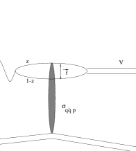
Figure 1: Scheme for vector meson production in the Color Dipole model.

The dynamics of the interaction between the $q\bar{q}$ pair and the proton are absorbed in the dipole cross section, $\sigma_{q\bar{q}-p}$. This approach to describing the scattering has been followed by many authors (see for example [3, 4, 5, 6, 7]), and is often called the Color Dipole model. In the version proposed by K. Golec-Biernat & M. Wüsthoff, the pair-proton cross section assumes the form

$$\sigma_{q\bar{q}-p}(Q,W,r)=\sigma_{0}\left(1-\exp\left[-\frac{r^{2}}{4R^{2}_{0}(Q^{2},W^{2})}\right]\right),\ \ \ \ \ \ {\rm where}$$ (1)

$$R_{0}(Q^{2},W^{2})=\frac{1}{{\rm{GeV}}}\left[\frac{1}{x_{0}}\frac{Q^{2}+4m_{q}^{2}}{Q^{2}+W^{2}}\right]^{\lambda/2}.$$ (2)

One important characteristic of this parameterization is that the cross section does not increase indefinitely with $r$, but “saturates” when $r$ increases beyond $R_{0}$. $R_{0}$ therefore defines a saturation radius, which depends on $Q^{2}$, $W^{2}$, and the mass of the quark/antiquark. The $W$ dependence of this cross section depends on the ratio $r/R_{0}$: for values of the ratio $\geq 1$, the $W$ dependence is approximately flat, while for small values, $\sigma_{q\bar{q}-p}$ scales approximately as $W^{2\lambda}$. We therefore expect a steeper $W$-dependence for heavy vector mesons relative to light vector mesons at a given $Q^{2},W^{2}$.

The three free parameters ($\sigma_{0}$, $\lambda$, $x_{0}$) in the expression above were determined via fits to DIS ($F_{2}$) data [1]. The total $\gamma^{*}p$ cross section is calculated as [8]:

$$\sigma_{L,T}(Q,W)=\int d^{2}\vec{r}\int dz|\Psi_{L,T}(Q,z,r)|^{2}\sigma_{q\bar{q}-p}(Q,W,r)$$ (3)

where $\Psi_{L,T}(Q,z,r)$ stands for the $q\bar{q}$ component of the wave function of a longitudinally (L) or transversely (T) polarized photon. The proton structure function $F_{2}$, the data from which is used in the extraction of the parameters, is related to $\sigma_{L,T}$ via

$$F_{2}(Q^{2},W^{2})=\frac{Q^{2}}{4\pi^{2}\alpha}(\sigma_{T}+\epsilon\cdot\sigma_{L}).$$ (4)

The numbers resulting from the fit are $\sigma_{0}$ = 23.03 mb, $\lambda$ = 0.288 and $x_{0}$ = 3.04$\times 10^{-4}$ if only three light quarks are assumed for the photon wavefunction, and $\sigma_{0}$ = 29.12 mb, $\lambda$ = 0.277 and $x_{0}$ = 0.41$\times 10^{-4}$ if one also considers charm.

In these fits the light quark ($u,d,s$) mass is used as a parameter and fixed to $m_{u,d,s}=140$ MeV; this average value was necessary to allow the model to give rough agreement with the total photoproduction cross section. The charm quark mass used in the calculations is discussed below.

The model has been applied in the calculation of other inclusive processes, and has provided good results with no extra parameters. For example, it gives the qualitatively correct behavior for the quantity $dF_{2}/d\ln{Q^{2}}$ at low $Q^{2}$. Furthermore the diffractive cross section $\sigma^{diff}$ is reasonably reproduced in the model [2].

Our aim in this work is to test the model for exclusive processes. We analyze the model in photo- and electroproduction of $J/\Psi,\ \rho$ and $\phi$ mesons. We first describe the calculations, and then compare the results with published HERA data.

2 Vector Meson Production

In this section we give the principal formulae for the process $\gamma^{(*)}p\rightarrow Vp$ in the context of Color Dipole model. One writes the amplitude for the process as $A=\ <V\ |\ \sigma_{q\bar{q}-p}\ |\ \gamma^{(*)}>$, where $|V>$ is the vector meson wavefunction and $|\gamma^{*}>$ is the $q\bar{q}$ component of the $\gamma^{*}$ wavefunction. In the $(\vec{r},z)$ representation $A$ is given by [9]

$$A_{L,T}=\int_{0}^{1}dz\int d^{2}\vec{r}\ \Psi_{V}^{*L,T}(r,z)\ \sigma_{q\bar{q}-p}(Q,W,r)\ \Psi_{\gamma}^{L,T}(Q,r,z)$$ (5)

where $\sigma_{q\bar{q}-p}(Q,W,r)$ is the cross section for the pair-proton interaction. The forward scattering cross section is then given by

$$\frac{d\sigma}{dt}|_{t=0}=\frac{\ |A|^{2}}{16\pi}.$$ (6)

Since the model does not incorporate any $t$ dependence we assume the ordinary exponential $t$ dependence, $d\sigma/dt\simeq Ce^{-B|t|}$ observed in the data, so that the total cross section is given by

$$\sigma(\gamma p\rightarrow Vp)=\frac{1}{B}\frac{d\sigma}{dt}|_{t=0}=\frac{1}{B}\frac{|A|^{2}}{16\pi}.$$ (7)

The $q\bar{q}$ component of the photon wave function is quite well known [10]. For photons with longitudinal polarization we have

$$\Psi_{\gamma}^{L}=\frac{\sqrt{N_{c}}}{(2\pi)^{3/2}}\sqrt{4\pi\alpha}\ e_{q}\ 2Qz(1-z)\phi^{\gamma}(z,r)\delta_{\lambda_{1},-\lambda_{2}}$$ (8)

and for transverse polarization

$$\Psi_{\gamma}^{T}=\frac{\sqrt{N_{c}}}{(2\pi)^{3/2}}\sqrt{4\pi\alpha}\ e_{q}\{m_{q}\left(\begin{array}[]{l}\mp 1\\ -i\end{array}\right)\phi^{\gamma}(r,z)\delta_{\lambda_{1},\lambda_{2}}+$$ (11)

$$\left(\begin{array}[]{l}i(2z-1)\hat{b}_{x}\mp\hat{b}_{y}\\ \pm\hat{b}_{x}+i(2z-1)\hat{b}_{y}\end{array}\right)\frac{\partial\phi^{\gamma}(r,z)}{\partial r}\delta_{\lambda_{1},-\lambda_{2}}\}.$$ (14)

In the expressions above $N_{c}$ is the number of colors, $e_{q}(m_{q}$) is the quark charge (mass), $\lambda_{1,2}$ are the helicities of the $q$ and $\bar{q}$, and $\phi^{\gamma}(r,z)$ is the photon spatial wave function given by

$$\phi^{\gamma}(r,z)=K_{0}(r\sqrt{Q^{2}z(1-z)+m_{q}^{2}}\ ).$$ (15)

In analogy with the photon wave function one can write for the longitudinally polarized vector mesons

$$\Psi_{V}^{L}=-2M_{V}\phi^{V}(z,r)\delta_{\lambda_{1},-\lambda_{2}}$$ (16)

and for the transversely polarized vector mesons

$$\Psi_{V}^{T}=\frac{m_{q}}{z(1-z)}\left(\begin{array}[]{l}\pm 1\\ -i\end{array}\right)\phi^{V}(z,r)\delta_{\lambda_{1},\lambda_{2}}+$$ (19)

$$\frac{1}{z(1-z)}\left(\begin{array}[]{l}i(2z-1)\hat{b}_{x}\mp\hat{b}_{y}\\ \pm\hat{b}_{x}+i(2z-1)\hat{b}_{y}\end{array}\right)\frac{\partial\phi^{V}(r,z)}{\partial r}\delta_{\lambda_{1},-\lambda_{2}}.$$ (22)

In the case of the vector mesons, the spatial part of the wave function is not known, and some hypothesis must be made. In the following sections we discuss the vector meson wave functions.

3 $J/\Psi$ wave function

Since the internal motion is slow for heavy quarkonium, we can choose a non-relativistic wave function. For transversely polarized photons, $J_{z}=\pm 1$. If we assume that the orbital angular momentum of the quark and antiquark in the $J/\psi$ is 0, then $S_{z}=\pm 1$. This implies $\lambda_{1}=\lambda_{2}$, and the second term in Eq. (12) disappears (see also  [11]). We analyze some possible wave functions in $(z,k_{t})$ space, and then calculate the $(z,r)$ wavefunction using a 2-D Fourier transform,

$$\phi_{V}(r,z)=\int\frac{d^{2}k_{t}}{4\pi^{2}}\ \phi_{V}(z,k_{t})e^{ir\cdot k_{t}}\;\;.$$ (23)

3.1 $\delta$-function

The simplest case one can have is to consider that the $q$ and $\bar{q}$ have the same longitudinal momentum fraction and that the transverse momentum is very small. In terms of a $(z,k_{t})$ space wavefunction, this hypothesis yields

$$\phi_{V}(z,k_{t})=K\ \delta(z-1/2)\delta^{2}(k_{t})\;\;.$$ (24)

The only free parameter is the normalization, $K$. It can be determined if we fix the partial width for $J/\psi\rightarrow e^{+}e^{-}$ to the experimentally measured value.

$$\Gamma^{V}_{e^{+}e^{-}}=\frac{32\pi\alpha^{2}e_{q}^{2}}{M_{V}}\ |\int dz\int\frac{d^{2}k_{t}}{8\pi^{3/2}}\Psi_{V}(z,k_{t})|^{2}$$ (25)

resulting in

$$K=\frac{1}{2M_{V}}\frac{8\pi^{3/2}}{e_{q}\alpha}\sqrt{\frac{\Gamma^{V}_{e^{+}e^{-}}M_{V}}{32\pi}}.$$ (26)

The wave function in the $(r,z)$ space representation, obtained via Eq. (23), is then

$$\phi_{V}(r,z)=\frac{1}{2M_{V}}\frac{\sqrt{4\pi}}{e_{q}\alpha}\sqrt{\frac{\Gamma^{V}_{e^{+}e^{-}}M_{V}}{32\pi}}\delta(z-1/2).$$ (27)

The full expression for longitudinal and transverse wave functions is obtained by inserting the expression above in Eqs. (11) and (12).

3.2 Gaussian function

Another possibility is to consider again the same longitudinal momentum fraction for both $q$ and $\bar{q}$ but now we assume that some small transverse momentum is allowed inside the $J/\Psi$. Following [12], we use a Gaussian distribution around zero and the wave function reads

$$\phi_{V}(z,k_{t})=K\ \delta(z-1/2)\exp(-a\frac{k^{2}_{t}}{m_{c}^{2}}).$$ (28)

We take for $a$ the value obtained from lattice QCD calculations, $a=4.68$ and $m_{c}=$1.43 GeV.

Again the normalization is obtained from the decay width,

$$K=\frac{a}{m_{c}^{2}}\frac{1}{2M_{V}}\frac{8\pi^{3/2}}{e_{q}\alpha}\sqrt{\frac{\Gamma^{V}_{e^{+}e^{-}}M_{V}}{32\pi}}$$ (29)

and the $(r,z)$ representation of the wave function comes from the Fourier transform.

3.3 Double-Gaussian function

We propose now that not only the transverse momentum may have some distribution but also the longitudinal momentum fraction has a Gaussian distribution around 1/2, resulting in

$$\phi_{V}(z,k_{t})=K\ \exp[-c^{2}(z-1/2)^{2}]\exp(-a\frac{k^{2}_{t}}{m_{c}^{2}}).$$ (30)

Now the wave function has one extra parameter, $c$. However, one extra constraint is available since now the wave function can be normalized. From the decay width

$$K=\frac{a}{m_{c}^{2}}\frac{1}{2M_{V}}\frac{8\pi^{3/2}}{e_{q}\alpha}\sqrt{\frac{\Gamma^{V}_{e^{+}e^{-}}M_{V}}{32\pi}}\frac{c}{\sqrt{\pi}\ {\rm erf}(c/2)},$$ (31)

and from the normalization condition,

$$\frac{N_{c}}{2\pi}\int_{0}^{1}\frac{dz}{z^{2}(1-z)^{2}}\int d^{2}\vec{r}\{m_{c}^{2}|\phi(r,z)|^{2}\}=1$$ (32)

we get $c^{2}=27.2$. In this way the $(r,z)$ representation of the wave function is obtained via the Fourier transform with no free parameters.

4 Light meson wave functions

For the light mesons, a relativistic approach must be used. We follow the procedure outlined in [13, 14], where one writes the wave function in terms of the lightcone invariant variable $\vec{p}^{\ 2}$ (3-momentum of the quark in the non-relativistic limit),

$$\vec{p}^{\ 2}=\frac{1}{4}(M^{2}-4m_{q}^{2}),\ \ \ \ \ \ \ \ \ M^{2}=\frac{m_{q}^{2}+k_{t}^{2}}{z(1-z)}.$$ (33)

In this expression $M$ is the invariant mass of the $q\bar{q}$ system, and $m_{q}=140$ MeV is the quark mass. Again a Gaussian form is applied, now in the $\vec{p}$ variable,

$$\phi(\vec{p})=K\ (2\pi R^{2})^{3/2}\exp\left[-\frac{1}{2}p^{2}R^{2}\right].$$ (34)

The value of $R$ was fixed by requiring that the exponential gives a value of $1/e$ for $M=M_{V}$. This yielded

$R^{2}_{\rho}=15.5$ GeV^-2,

$R^{2}_{\phi}=8.3$ GeV^-2.

Using Eqs. (23) above one obtains the wave function in the $(z,k_{t})$ representation, and through Eq. (13)

$$\phi(r,z)=K\ 4z(1-z)\sqrt{2\pi R^{2}}\exp[-\frac{m_{q}^{2}R^{2}}{8z(1-z)}]\exp[-\frac{2z(1-z)r^{2}}{R^{2}}]\exp[-\frac{m_{q}^{2}R^{2}}{2}]\;\;.$$ (35)

The normalization factor $K$ is determined from the normalization condition, so that once again there are no free parameters.

5 Results

We have fixed the $u,d,s$ quark masses to 140 MeV, as in [1], and use either the three or four quark parameters given in the introduction (for the $J/\psi$ case, only the four quark parameters are used). For the slope $B$ (see Eq. (7)) we use a parameterization to experimental data, given by  [15]

$$B=0.60\left(\frac{14}{(Q^{2}+M_{V}^{2})^{0.26}}+1\right)\;\;.$$ (36)

This parameterization is used for all the vector mesons.

5.1 $J/\Psi$ production

In Fig. 2, the $W$ dependence of the $\gamma^{*}p$ cross section for $J/\Psi$ elastic production is shown for various values of $Q^{2}$. It can be seen that even for the simplest wave function utilized ($\delta$-function, dotted line) the $W$ dependence predicted by the model is in agreement with the data, although for photoproduction the normalization is not very good for this wave function. For the more complicated forms we obtain good agreement to HERA data both in shape and in normalization. Note that the value of $R_{0}$ in Eq. (2) is never very small in $J/\psi$ production because of the presence of the charm quark mass, implying that we are far from the low $Q^{2}$ or high $W$ saturation regions. The $W$ dependence is then given to good approximation by $\sigma_{\gamma^{*}p\rightarrow J/\psi p}\propto W^{4\lambda}$.

Figure 2: The W-dependence of elastic $J/\Psi$ production as a function of $Q^{2}$. Open circles are ZEUS data [17, 18] and solid circles H1 data [19, 20]. The dotted lines correspond to calculations using the $\delta$-function wave function, the dashed lines to calculations using a single Gaussian, and the solid lines to the double Gaussian wavefunction as discussed in the text. The $Q^{2}$ values, in units of GeV², are indicated in the figure. The data and calculations have been scaled by the values given for clarity of presentation.

Fig. 3 gives the ratio of the longitudinal to transverse cross sections, $\sigma_{L}/\sigma_{T}$, for fixed $W$ as a function of $Q^{2}$ (upper plot), and for fixed $Q^{2}$ as a function of $W$ (lower plot). Due to the delta function in $z$ for the $\delta$ and Gaussian wave functions, the integration over $d^{2}rdz$ is the same for transverse and longitudinal amplitudes, up to a constant factor. In this case the model dependence for $R$ disappears and one gets just $R=Q^{2}M_{V}^{2}/(16m_{q}^{4})$. The dotted and dashed curves are therefore superimposed in Fig. 3. For the double Gaussian case this does not occur; $A_{L}$ is peaked near $z=1/2$ and the $Q^{2}$ growth is damped relative to $A_{T}$. It is clear that the $Q^{2}$ dependence of $R=\sigma_{L}/\sigma_{T}$ is quite sensitive to the vector meson wavefunction, while there is little sensitivity in the $W$ dependence. The data favor the double Gaussian wavefunction.

Figure 3: Ratio $R=\sigma_{L}/\sigma_{T}$ for elastic $J/\Psi$ electroproduction. The dotted and dashed lines (superimposed) correspond to the $\delta$ and single Gaussian wave functions. The solid lines are calculated with Double Gaussian wave function. The upper plot gives the $Q^{2}$ dependence at fixed $W=90$ GeV. The lower plot gives results versus $W$ for $Q^{2}$ = 6.2 GeV² (upper curves), and $Q^{2}$ = 0.45 GeV² (lower curves). The open circles are ZEUS data [18] and the solid circles are H1 data [20].

5.2 $\rho$ production

The comparisons to data for elastic $\rho$ production are given in Figs. 4-6. The lighter mass of the $\rho$ allows the cross sections to enter the saturation region ($r\sim R_{0}$), and the $W$ dependence is a strong function of $Q^{2}$, as seen in Fig. 4. The two sets of curves on the graph give the results for three quark (dashed) and four quark (solid) parameter sets. The normalization of the cross sections is not particularly good, and the $Q^{2}$ dependence is also not well reproduced, although the 3 parameter set does a better job of reproducing the $Q^{2}$ dependence. Note that the normalization is affected both by the choice of $\rho$ wavefunction and by the assumed $B$ values. However, the observed change of the $W$ dependence is rather well reproduced. This is quantified in Fig. 5, where the power $\delta$ from a fit of the $W$ dependence with a form $\sigma_{\gamma^{*}p\rightarrow\rho p}\propto W^{\delta}$ is compared with data.

Figure 4: The $W$-dependence of elastic $\rho$ production as a function of $Q^{2}$ compared with recent ZEUS [21, 18] and H1 [22, 23] data. The $Q^{2}$ values are given in the plot. The solid lines are for the four quark parameters, while the dashed lines are for the three quark parameter sets.

Figure 5: The $W$-dependence of elastic $\rho$ production as a function of $Q^{2}$, compared with recent ZEUS [18] (open circles) and H1 [23] (solid circles) data. The solid line is the result using the four flavor parameter set, and the dashed curve is the result using the three flavor parameter set.

The dependence of $R=\sigma_{L}/\sigma_{T}$ on $Q^{2}$ at fixed $W$ is shown in Fig. 6, as is the $W$-dependence at fixed $Q^{2}$. The model, with the simple wavefunction chosen, gives a good representation of the data. In this case, the model predicts a small variation of $R$ with $W$.

Figure 6: $R$ dependence on $Q^{2}$ and $W$ in elastic $\rho$ production. The upper plot gives the $Q^{2}$ dependence at fixed $W=75$ GeV, while the lower plot gives the $W$ dependence at the $Q^{2}$ values indicated in the plot. The open circles are ZEUS data [18] and the solid circles H1 data [23].

5.3 $\phi$ production

For the $\phi$ meson, we compare the predicted $W$ dependence for $\gamma^{*}p\rightarrow\phi p$ as a function of $Q^{2}$ with data in Fig. 7 and $R$ versus $Q^{2}$ at fixed $W$, as well as $R$ versus $W$ at fixed $Q^{2}$ in Fig. 8. The normalization of the cross section is too high given the chosen wavefunction and parameterization for $B$, but the $R$ dependence on $Q^{2}$ is in reasonable agreement with the available data.

Figure 7: $\sigma_{\gamma^{*}p\rightarrow\phi p}$ as a function of $W$ for different $Q^{2}$, compared with ZEUS data [24]. The solid lines are for the four flavor parameter set, while the dashed lines are for the three flavor parameter set.

Figure 8: Ratio of longitudinal over transverse cross sections in $\phi$ production. The upper plot shows the $Q^{2}$ dependence at fixed $W$, while the lower plot shows the $W$ dependence at fixed $Q^{2}$. The solid lines are for the four flavor parameter set, while the dashed lines are for the three flavor parameter set. The data are from ZEUS [24] and H1 [25].

6 Summary and Conclusions

We have used the Golec-Biernat Wüsthoff model to calculate the cross section for exclusive vector meson production in $ep$ scattering. The model gives the correct $W$ dependence for both photo- and electroproduction of $J/\psi$ mesons. This feature can be attributed to the model because it is observed even when a very simple wave function is employed. This was not unexpected, since the model reproduces the pQCD expectations for the $Q^{2}$ and $W$ dependence of $\sigma_{\gamma^{*}p\rightarrow\psi p}$ when the dipole size is small compared to the “saturation radius”. Perhaps more surprising is the fact that a simple $J/\psi$ wave function (double Gaussian) also gives good results for the normalization of the wavefunction as well as for the $Q^{2}$ dependence of $R=\sigma_{L}/\sigma_{T}$.

For $\rho$ and $\phi$ production, the $W$ dependence changes dramatically as we go from photoproduction to DIS. The change in the $W$ dependence versus $Q^{2}$ calculated using a simple wavefunction can reproduce the data reasonably well. The behavior of $R$ versus $Q^{2}$ and $W$ is also in reasonable agreement with the data. However, the normalization of the cross section is not in agreement with the data, and the discrepancy with data varies with $Q^{2}$. This problem can be attributed to the lack of knowledge of the wave function and perhaps also in part to the change in $t$-slope with $Q^{2}$ (this slope is needed to calculate the total cross section).

The proton rest frame description of $ep$ scattering gives a simple and intuitive picture of low $Q^{2}$ and small-$x$ scattering. Golec-Biernat and Wüsthoff have shown, using a three parameter parametrization for the $q\bar{q}-p$ scattering cross section, that the total as well as the diffractive cross sections can be well described. We find that the the model can also describe many of the features of exclusive vector meson production.

Acknowledgments

The authors would like to thank the U.S. National Science Foundation and the Brazilian agency FAPESP for support during the period of this study. One of us, M.S., would also like to thank Columbia University for its hospitality during this period. We are grateful for useful discussions with H. Abramowicz, Z. Chen, R. Covolan, J. Gravelis, H. Kowalski, R. Mawhinney, A. Mueller, J. Nemchik, E. Predazzi, F. Sciulli, and M. Strikman.

References

- [1] K. Golec-Biernat, M. Wüstoff, Phys. Rev. D 59 (1999) 014017.
- [2] K. Golec-Biernat, M. Wüstoff, Phys. Rev. D 60 (1999) 114023.
- [3] A. H. Mueller, Nucl. Phys. B 335 (1990) 115.
- [4] N. Nikolaev, B. G. Zakarov, Z. Phys. C 49 (1990) 607.
- [5] N. Nikolaev, E. Predazzi, B. G. Zakharov, Phys. Lett. B 326 (1994) 161.
- [6] S. J. Brodsky et al. Phys. Rev. D 50 (1994) 3134.
- [7] E. Gotsman, E. Levin, U. Maor, Phys. Lett. B 425 (1998) 369.
- [8] J. R. Forshaw and D. A. Ross, QCD and the Pomeron, Cambridge University Press, 1986.
- [9] N. N. Nikolaev and B. G. Zakharov, Z. Phys. C 53 (1992) 331.
- [10] N.N. Nikolaev, B.G. Zakharov, Z.Phys. C49 (1991) 607.
- [11] M. Wüsthoff and A. D. Martin, J. Phys. G 25, R309 (1999).
- [12] M.G. Ryskin, R.G. Roberts, A.D. Martin, E.M. Levin, Z. Phys. C 76, 231 (1997).
- [13] L. Frankfurt, W. Koepf, M. Strikman, Phys. Rev. D 54 (1996) 3194.
- [14] J. Nemchik, N.N. Nikolaev, E. Predazzi, B.G. Zacharov Z. Phys. C 75 (1997) 71.
- [15] Bruce Mellado, private communication.
- [16] L. Frankfurt, W. Koepf, M. Strikman, Phys. Rev. D 57 (1998) 512.
- [17] ZEUS Collab., M. Derrick et al., Z. Phys. C 75 (1997) 215.
- [18] ZEUS Collab., J. Breitweg et al., Eur. Phys. J. C 6 (1999) 603.
- [19] H1 Collab., C. Adloff et al., Phys. Lett. B 483 (2000) 23.
- [20] H1 Collab., C. Adloff et al., Eur. Phys. J. C 10 (1999) 373.
- [21] ZEUS Collab., J. Breitweg et al., Eur. Phy. J. C 2 (1998) 247.
- [22] H1 Collab., S. Aid et al., Nucl. Phys. B 463 (1996) 3.
- [23] H1 Collab., C. Adloff et al., Eur. Phys. J. C 13 (2000) 371.
- [24] ZEUS Collab., M. Derrick et al., Phys Lett. B 380 (1996) 220.
- [25] H1 Collab., C. Adloff et al., Phys. Lett. B 483 (2000) 360.