$S$-matrix Bases and Relation between
$\pi\pi$-Scattering and Production Amplitudes

1 Purpose of This Talk

The (partial $S$-wave) amplitude of $\pi\pi$-production ${\cal F}_{\pi\pi}(s)$ for $\sqrt{s}\stackrel{{\scriptstyle<}}{{\scriptstyle\sim}}1$GeV ($\sqrt{s}$ being total mass of the $\pi\pi$ system), obtained in most experimental processes such as $pp\to pp(\pi\pi)$, $\psi^{\prime}\to J/\psi(\pi\pi)$, $\mathchar 28935\relax^{(n)}\to\mathchar 28935\relax^{(m)}(\pi\pi)$ and $p\bar{p}\to(\pi\pi)\pi$ had been exceptionally crudely and not duely treated[1] under the influence of “universality argument.” It says[2] that ${\cal F}_{\pi\pi}(s)$ must be proportional to the (partial $S$-wave) amplitude of $\pi\pi$-scattering ${\cal T}_{\pi\pi}(s)$ as

$${\cal F} = \alpha(s){\cal T},$$ (1.1)

where the $\alpha(s)$ is, due to the final state interaction (FSI) theorem, real, and is moreover, due to analyticity, slowly varying. Accordingly the structure of ${\cal F}$ obtained in any experiment should be the same as that of ${\cal T}$. In most of the conventional works following to this argument, the analyses of ${\cal F}_{\pi\pi}(s)$ in this region $\sqrt{s}\stackrel{{\scriptstyle<}}{{\scriptstyle\sim}}1$GeV, where the ${\cal T}(s)$ was investigated comparatively well, had become just fitting procedure of experimentally obtained ${\cal F}_{\pi\pi}$ to ${\cal T}_{\pi\pi}$ through a respective function $\alpha(s)$ expressed in terms of physically meaningless arbitrary parameters. Since there was, at that time, observed no structure corresponding directly to the resonance with relevant mass in ${\cal T}_{\pi\pi}$, the large concentration of iso-scalar $S$-wave $2\pi$ events (with mass 400$\sim$800MeV) frequently observed in the many production channels had been conventionally treated as a mere background. Thus the $\sigma$-particle, which was[5] anticipated both theoretically and phenomenologically in many works, had been disappeared for almost 20 years in the list of PDG before its 1996 edition.

The purpose of present talk is to point out[1] that the FSI theorem and the analyticity requirement should be applied on the $S$-matrix element with the “right bases” and that the effective $\alpha(s)$ derived in a field theoretical model with right quark-physical bases is not slowly varying function, that is, the above universality argument which dismisses quark picture is not correct.

Thus the analyses following the argument is meaningless, and the ${\cal F}(s)$ should be, in principle, treated independently from ${\cal T}(s)$. Actually we made analyses[4] on the various production processes along this line, and obtained strong evidences of $\sigma$-meson production.

2 Phenomenological Methods of Analyses of Amplitudes

In the following we summarize both methods in conventional and our analyses and compare with them.

[Conventional Method]

$${\cal T}(s) = {\cal K}(s)/(1-i\rho{\cal K}(s)),$$ (2.1)

$${\cal F}(s) = {\cal P}(s)/(1-i\rho{\cal K}(s)),\ \ {\cal P}(s)\equiv\alpha(s){\cal K}(s).$$ (2.2)

These forms in Eqs. (2.1) and (2.2) are generally derived from the requirement of elastic unitarity and of FSI theorem. However, the concrete forms of ${\cal K}(s)$ and ${\cal P}(s)$ (or $\alpha(s)$) are model-dependent. In the conventional method these are expressed in terms of arbitrary parameters with no physical meanings. For example, in the original analysis[2] they choose a form, with arbitrary parameters, $\alpha_{n}$’s, and with the experimentally fixed zero-point of ${\cal T}(s)$, $s_{0}^{\cal T}$, as

$$\alpha(s) = \sum_{n}\alpha_{n}s^{n}/(s-s_{0}^{\cal T}).$$ (2.3)

[Our Method]
Interfering Amplitude (IA) Method:[7]

$${\cal T}(s) : S=S^{\rm R}S^{\rm BG},\ \ S^{\rm R}=S^{\sigma}S^{f};\ \ \ S^{(r)}=e^{2i\delta^{(r)}}\Rightarrow\ \delta=\delta^{\sigma}+\delta^{f}+\delta^{\rm BG};$$

$$S^{(r)} \equiv 1+2ia^{(r)},\ \ \ a^{(r)}\equiv\sqrt{\rho}{\cal T}^{(r)}\sqrt{\rho};\ \ \ a=a^{\rm R}+a^{\rm BG}+2ia^{\rm R}a^{\rm BG},$$

$$a^{\rm R} = a^{\sigma}+a^{f}+2ia^{\sigma}a^{f},\ \ \ a^{\sigma}=a_{\rm BW}^{\sigma}\equiv\frac{\sqrt{s}\mathchar 28928\relax_{\sigma}(s)}{\lambda_{\sigma}-s}\ \ {\rm etc.}$$ (2.4)

Variant Mass and Width (VMW) Method:

$${\cal F}(s) : {\cal F}=\frac{r_{\sigma}e^{i\theta_{\sigma}}}{\lambda_{\sigma}-s}+\frac{r_{f}e^{i\theta_{f}}}{\lambda_{f}-s}+r_{\rm BG}e^{i\theta_{\rm BG}},\ \ \ \lambda_{\sigma}\equiv m_{\sigma}^{2}-i\sqrt{s}\mathchar 28928\relax_{\sigma}(s)\ \ {\rm etc};\ \ \ \$$ (2.5)

where all terms and contained parameters have respective direct physical meanings. In Eqs. (2.4) and (2.5) we give the formulas in the relevant case with two resonances, $\sigma$ and $f_{0}(980)$. Our ${\cal T}$ given in Eq.(2.4) satisfies automatically the elastic unitarity, while Eq. (2.5) is consistent with the $S$-matrix unitarity. The FSI theorem gives some constraints among the $r_{i}$ and $\theta_{i}$ contained in ${\cal F}$. Here, it is to be noted that our ${\cal T}$ and ${\cal F}$ given above are also rewritten[1] into the general forms Eqs. (2.1) and (2.2). (See the following sections.)

3 Strong Interaction and Bases of $S$-matrix

Before going into detailed discussions on the relevant problem, it is necessary to consider about rather general and fundamental physical situation:
The strong interaction is “residual interaction” of QCD among color-neutral bound states $\bar{\phi}$ of quarks (antiquarks) $q(\bar{q})$ and gluons $g$.

$${\cal H}^{\rm str}(\bar{\phi}_{i}) = {\rm resid.\ int.\ among\ }\bar{\phi}_{i}^{\prime}{\rm s}.$$ (3.1)

The unitarity of $S$ matrix is guaranteed by hermiticity of interaction Hamiltonian,

$$SS^{\dagger} = S^{\dagger}S=1\longleftarrow{\cal H}^{{\rm I}\dagger}={\cal H}^{\rm I}.$$ (3.2)

It should also be noted that the basic fields are stable bound states $\bar{\phi}_{i}$’s and that the complete set of bases of $S$-matrix is given as a configuration space of these multi-$\bar{\phi}_{i}$ states. Here it is instructive to remember the old history of strong interaction of the $\pi N$ system.

Table I: Bases of $S$-matrix — Old History of Pictures on Strong Interaction of $\pi N$ System

	Chew-Low	Theory	After quark physics
Switch off
${\cal H}^{\rm I}$	Basic fields	$\pi$, $N$	$\bar{\pi}=(q\bar{q})$, $\bar{N},\ \underline{\bar{\mathchar 28929\relax}=(qqq)}$ “zero” $\mathchar 28928\relax$
Switch on
${\cal H}^{\rm I}$	Resonance	$\mathchar 28929\relax$ $(N\pi+N\pi\pi)$	$\pi_{\rm phys.}$, $N_{\rm phys.}$; $\underline{\mathchar 28929\relax_{\rm phys.}}$ “finite” $\mathchar 28928\relax$
	Compl. Set
	of $S$-bases	$|\pi\rangle$, $|N\rangle$, $|\pi N\rangle$, $\cdots$	$|\bar{\pi}\rangle$, $|\bar{N}\rangle$, $\underline{|\bar{\mathchar 28929\relax}\rangle}$, $|\bar{\pi}\bar{N}\rangle$, $\underline{|\bar{\pi}\bar{\mathchar 28929\relax}\rangle}$, $\cdots$

Table II: Present problem

	Unitary Chiral approach	Ours (L$\sigma$M, NJLM)
Basic fields	$\bar{\pi}$	$\bar{\pi}$; $\bar{\sigma}$, $\bar{f}$=$(q\bar{q})$ “zero” $\mathchar 28928\relax$
Resonance	$\sigma(\pi\pi)$, $[f(K\bar{K})]$	$\ \ \ \sigma_{\rm phys.}$  $f_{\rm phys.}$   “finite” $\mathchar 28928\relax$
Compl. set of $S$-bases	$|\pi\rangle$, $|\pi\pi\rangle$, $\cdots$	$|\bar{\pi}\rangle,\ |\bar{\sigma}\rangle$, $|\bar{f}\rangle,\ |\bar{\pi}\bar{\pi}\rangle$

As is summarized in Table I, there are the two pictures; the one is of Chew-Low theory and the other one is of quark physics. In the former the basic fields are only $\pi$ and $N$, while in the latter they include also the bare $\bar{\mathchar 28929\relax}$ field with zero-width as a three-quark stable bound-state $\bar{\mathchar 28929\relax}$=$(qqq)$. After switching on ${\cal H}_{\rm I}^{\rm str.}$, in the former the physical $\mathchar 28929\relax$-particle appears as a resonance of $\pi N$ system, while in the latter the $\bar{\mathchar 28929\relax}$ becomes $\mathchar 28929\relax_{\rm phys.}$ with finite width. These two pictures may be phenomenolgically consistent with each other in so far as concerned with interactions of the $\pi N$ system. However, we recognize presently the latter as a true one from the general and fundamental viewpoint.

In the present problem of the $\pi\pi$ system with two resonant particles $\sigma_{\rm phys.}(600)$ and $f_{0,{\rm phys.}}(980)$ the similar situation as is summarized in Table II may be valid. That is, the two pictures, the unitary chiral approach and our quark-picture based on the linear $\sigma$ model (L$\sigma$M) and on the NJL model, may be phenomenologically consistent. But we consider that the latter should be the very true one from the general and fundamental viewpoint.

4 Relation between Scattering and Production Amplitudes

[Field Theoretical Model]   In order to explain clearly the essential points of our problem we consider a simplified field theoretical model of the relevant system, where we should take the bare fields $\bar{\sigma}$ and $\bar{f}$ as well as the $\bar{\pi}$ as basic fields, and we set up the strong interaction Hamiltonian

$$H_{\rm int}^{\rm scatt}=\sum_{\alpha=\sigma,f}\bar{g}_{\alpha}\bar{\alpha}\pi\pi+\bar{g}_{\pi\pi}(\pi\pi)^{2},\ \ H_{\rm int}^{\rm prod}=\sum_{\alpha=\sigma,f}\bar{\xi}_{\alpha}\bar{\alpha}``P^{\prime\prime}+\bar{\xi}_{\pi\pi}\pi\pi``P^{\prime\prime},$$ (4.1)

where $\bar{g}$ and $\bar{\xi}$ are real coupling constants, and “P” denotes a relevant production channel. Taking into account the pion-loop effects due to the $H_{\rm int}^{\rm scatt}$, the stable bare states $\bar{\pi},\bar{\sigma}$ and $\bar{f}$ change into the physical states denoted as $\pi=(\bar{\pi})$, and $\sigma$ and $f$ with finite widths. Then we can derive the scattering and production amplitudes following the standard procedure of quantum field theory.

The general structure of ${\cal T}$ and ${\cal F}$ is shown schematically in Fig. 1, where shaded ellipses represent the final state interaction of the $2\pi$ system. It is to be noted that correctly both the mechanisms in Fig. 1 should be taken into account.

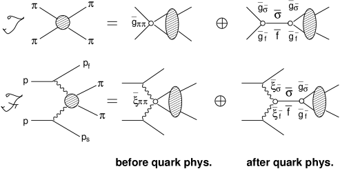
Fig. 1: The mechanism for scattering amplitude ${\cal T}$ and production amplitude ${\cal F}$. The second diagram should be correctly taken into account as well as the first, whereas only the first had been considered in the conventional treatment.

As a matter of fact, in the conventional treatment, where only the former is taken into account, the $\alpha(s)$ in Eq.(2.2) becomes

$$\alpha(s) = \bar{\xi}_{\pi\pi}/\bar{g}_{\pi\pi}={\rm const}.\ ,$$ (4.2)

which is surely a (most) slowly varying function with $s$.

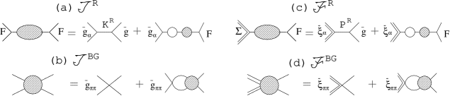
Fig. 2: Scattering and production mechanism in a simple field-theoretical model. The respective production amplitudes ${\cal F}^{(r)}$ are obtained, following the mechanism shown in the figures, by replacing the first $\pi\pi$-coupling constant $\bar{g}$ in ${\cal T}^{(r)}$ with the production coupling $\bar{\xi}$. The ${\cal F}$ amplitude obtained in this way automatically satisfies the FSI theorem.

In the previous work[1] resorting to the above model we have derived our methods of analyses, the IA method for ${\cal T}$ and the VMW method for ${\cal F}$, and shown their consistency with the FSI theorem. The obtained formulas of the amplitudes (derived as solutions of Schwinger-Dyson equations shown in Fig. 2 where (a) and (b) ( (c) and (d) ) correspond, respectively, to ${\cal T}^{R}$ and ${\cal T}^{BG}$ (${\cal F}^{R}$ and ${\cal F}^{BG}$)) are given for quantities defined in the general formulas, Eqs. (2.1), (2.2) and (2.4), as

$${\cal T} = \frac{{\cal K}^{R}+{\cal K}^{BG}}{(1-i\rho{\cal K}^{R})(1-i\rho{\cal K}^{BG})},\ \ \ {\cal K}=\frac{{\cal K}^{R}+{\cal K}^{BG}}{1-\rho^{2}{\cal K}^{R}{\cal K}^{BG}},$$ (4.3)

$${\cal F} = \frac{{\cal P}^{R}+{\cal P}^{BG}}{(1-i\rho{\cal K}^{R})(1-i\rho{\cal K}^{BG})},\ {\cal P}^{R}=\frac{{\cal P}_{\sigma}+{\cal P}_{f}}{1-\rho^{2}{\cal K}_{\sigma}{\cal K}_{f}},\ \ \ S^{(r)}\equiv\frac{1+i\rho{\cal K}^{(r)}}{1-i\rho{\cal K}^{(r)}}$$ (4.4)

$${\cal T} = {\cal T}^{R}(1+i\rho{\cal T}^{BG})+{\cal T}^{BG}(1+i\rho{\cal T}^{R}),\ \ {\cal F}={\cal F}^{R}(1+i\rho{\cal T}^{BG})+{\cal F}^{BG}(1+i\rho{\cal T}^{R})$$

$${\cal K}^{R} = \frac{{\cal K}_{\sigma}+{\cal K}_{f}}{1-\rho^{2}{\cal K}_{\sigma}{\cal K}_{f}},\ \ \ {\cal K}_{\alpha}=\frac{\bar{g}_{\alpha}^{2}}{\bar{m}_{\alpha}^{2}-s},\ \ (\alpha=\sigma,f),\ \ \ {\cal K}^{BG}=\bar{g}_{\pi\pi}$$ (4.5)

$${\cal P}_{\alpha} = \frac{\bar{\xi}_{\alpha}\bar{g}_{\alpha}}{m_{\alpha}^{2}-s};\ \ {\cal P}^{BG}=\bar{\xi}_{\pi\pi},\ \ \ S^{R}=\mathchar 28933\relax_{\alpha=\sigma,f}\frac{\lambda_{\alpha}^{*}-s}{\lambda_{\alpha}-s},\ \ \ S^{BG}=\frac{1+i\rho\bar{g}_{\pi\pi}}{1-i\rho\bar{g}_{\pi\pi}},\ \ \ \ \ \$$ (4.6)

where the formulas given in Eqs. (4.3) and (4.4) are rather generally derived following the mechanism of Fig. 2, while those in Eqs.(4.5) and (4.6) are derived depending on our choice of ${\cal H}_{\rm int}$ (4.1) in the “bare-state representation.” These formulas of ${\cal T}$ and ${\cal F}$ are rewritten into the forms of Eq.(2.4) and Eq.(2.5), respectively, in the “physical state representation.” The consistency with the FSI theorem of these amplitudes ${\cal F}$ and ${\cal T}$ is easily seen from Eqs.(4.3) and (4.4), since ${\cal K}$ and ${\cal P}$ are real and their phases come only from their common denominator $(1-i\rho{\cal K}^{R})(1-i\rho{\cal K}^{BG})$. The above amplitudes lead to

$$\alpha(s) = \frac{\bar{\xi}_{\sigma}\bar{g}_{\sigma}(m_{f}^{2}-s)+\bar{\xi}_{f}\bar{g}_{f}(m_{\sigma}^{2}-s)+\bar{\xi}_{\pi\pi}((m_{\sigma}^{2}-s)(m_{f}^{2}-s)-\rho^{2}\bar{g}_{\sigma}^{2}\bar{g}_{f}^{2})}{\bar{g}_{\sigma}^{2}(m_{f}^{2}-s)+\bar{g}_{f}^{2}(m_{\sigma}^{2}-s)+\bar{g}_{\pi\pi}((m_{\sigma}^{2}-s)(m_{f}^{2}-s)-\rho^{2}\bar{g}_{\sigma}^{2}\bar{g}_{f}^{2})},\ \ \ \$$ (4.7)

which is represented in terms of all physically meningful parameters. This has a form in contradistinction to the choice Eq.(2.3), and is not a slowly varying function. In our method the large event concentration mentioned in §1 is directly understood as results of $\sigma$-production by taking as $\bar{\xi}_{\sigma}/\bar{g}_{\sigma}\stackrel{{\scriptstyle>}}{{\scriptstyle\sim}}\bar{\xi}_{f}/\bar{g}_{f}\gg\bar{\xi}_{\pi\pi}/\bar{g}_{\pi\pi}\approx 0$ .

[Phenomenological Analyses]   In the actual analyses of ${\cal T}$ and ${\cal F}$ we have applied the IA method Eq.(2.4) and the VMW method Eq.(2.5), respectively, and obtained the strong evidence for existence of the light $\sigma$-meson: In the analyses of scattering amplitudes we have chosen the form of ${\cal T}_{BG}$ wih a hard core type $\delta_{BG}=-p_{1}r_{c}$ ($p_{1}$ being the pion momentum in the $2\pi$ rest frame). In the analyses of production amplitudes we have applied the two kinds of ${\cal F}$, the one which regards the constraints from the conventional FSI theorem and the other[8] which does not (, but is consistent with the $S$-matrix unitarity with the right quark-physical bases). An example of the former is given as Eq.(4.4) with ${\cal K}^{BG}=-({\rm tan}p_{1}r_{c})/\rho$ and ${\cal P}^{BG}=(\bar{\xi}_{2\pi}/r_{c}){\cal K}^{BG}$ instead of ${\cal K}^{BG}$ and ${\cal P}^{BG}$ given, respectively, in Eqs.(4.5) and (4.6).

5 Concluding Remarks

We have explained why the most conventional methods of analyses on ${\cal F}$ ($s\leq 1$GeV²) following the universality argument are physically meaningless and reviewed a new method of analysis taking quark-physical viewpoint correctly into account. As a result we may conclude; on experiment that production experiments have their own value independent of scattering experiments; on hadron phenomenology that its important task should be to extract the information on intrinsic quark-physical parameters such as $\bar{g}_{\alpha}$ and $\bar{m}_{\alpha}$; and on hadron theory that to explain their values from the fundamental theory, QCD or else, is one of its important purpose.

References

• [1] S. Ishida; M. Ishida, in proc. of WHS99, Frascati, 1999, ed. by T.Bressani, A. Feliciello and A. Filippi, Frascati Physics Series XV (1999), 85; 115. M. Ishida, S. Ishida and T. Ishida, Prog. Theor. Phys. 99 (1998), 1031.
• [2] M. R. Pennington, in proc. of Int. Conf. Hadron’ 95, Manchester UK, JulyΒ 1995, ed. by M. C. Birse, G.D. Lafferty and J.A.McGovern, (World Scientific, Singapore), p.3. K. L. Au, D. Morgan and M. R. Pennington ,Phys. Rev. D35 (1987), 1633.
• [3] M. Ishida, in proc. of WHS99; this proceedings.
• [4] T. Tsuru, this proceedings. K. Takamatsu, in proc. of Hadron97 at BNL, 1997, ed. by ed. by S.U. Chung and H.J. Willutzki, AIP conf. proc. 432.
• [5] T. Hatsuda and T. Kunihiro, Phys. Rep. 247 (1994), 221; this proceedings.
• [6] S. Ishida, M. Ishida and T. Maeda, Prog. Theor. Phys. 104 (2000), No.4.
• [7] S. Ishida et al., Prog. Theor. Phys. 95 (1996), 745.
• [8] M. Ishida, under preparation.