Optimized Perturbation Theory at Finite Temperature

1 Introduction

Experiments on ultra-relativistic heavy ion collisions at RHIC (the Relativistic Heavy Ion Collider) and LHC (the Large Hadron Collider) are being planned for the purpose of producing hot matter similar to that realized in the early universe. [2] In such a high-temperature ($T$) phase, quarks and gluons are deconfined and chiral symmetry is expected to be restored. The dynamics of such a phase transition from hadronic matter to a quark-gluon plasma is described by quantum chromodynamics (QCD) at finite $T$.

At present, there are two major calculational methods in QCD at finite $T$. One is the numerical simulations in lattice QCD. [3] This method has revealed that the restoration of chiral symmetry takes place at $T_{c}\sim 150$ MeV. For two flavors massless, the phase transition has been shown to be of second order. Analysis of the case with two light flavors and one medium-heavy quark, which corresponds to the real world, is also under study [4]. One of the disadvantages of lattice QCD is the difficulty of treating real-time excitations at finite $T$ in a straightforward way on the Euclidean lattice. [5]

Another method of treating QCD for $T\neq 0$ is based on the hard thermal loops resummation scheme (HTLRS). [6] It is generally known that naive perturbation theory breaks down at high temperature, [7, 8] even if the coupling constant is small. This is the reason that we must resum higher-order terms at finite $T$. HTLRS is a method of resuming the higher-order terms at high $T$ up to $O(gT)$ ($g$ is the QCD coupling constant) when the external momenta are $q\sim O(gT)$, a situation referred to as ‘soft’. With this method, physical quantities such as the soft gluon damping rate and the dilepton production rate have been calculated in the quark-gluon plasma (QGP) phase. [9] Since it is an effective resummation method which works only at high $T$, it cannot be applied to systems at low $T$. Also, in theories with spontaneous symmetry breaking (SSB), the loop expansion is more relevant than weak-coupling expansions, such as HTLRS.

To treat non-perturbative QCD effects at low energies, related to spontaneous symmetry breaking, effective models, such as the linear $\sigma$ model, have been developed. In such approaches, however, the serious problem of tachyonic poles appear [7], when one studies symmetry restoration at finite $T$. This problem shows up even below $T_{c}$, and it causes the breakdown of the thermal perturbation theory. Therefore, a resummation method applicable to a wide range of $T$ from low $T$ to high $T$ is required when effective models are studied.

To this time, several methods have been proposed for self-consistent resummation. [10] In these methods, there appear two major problems: [11] (i) appearance of $T$-dependent ultraviolet divergences, which makes the renormalizability non-trivial at finite $T$, and (ii) the breakdown of the Nambu-Goldstone (NG) theorem at finite $T$ when SSB occurs.

In Ref.[12], we have generalized the optimized perturbation theory (OPT) at finite $T$, which is a resummation method for solving the above mentioned problems. A similar idea has been proposed under the names of the delta-expansion, the variational perturbation theory, and so on. These ideas are applied to field theory at finite $T$ in Ref.[13] and [14]. In Ref.[13], the $O(N)$ $\phi^{4}$ theory with the principle of minimal sensitivity (PMS) (see §2.1) is studied. Since the formulation in that work is not based on the loop expansion, its authors could not prove renormalizability. Also, the NG-theorem is not satisfied in a straightforward way. In Ref.[14], $\lambda\phi^{4}$ theory with the fastest apparent convergence (FAC) condition (see §2.1) at high $T$ is studied. There, the renormalization up to the two-loop order is carried out in the symmetric phase. However, a rigorous definition of the method at higher orders and a proof of its renormalizability are not given.

Our method has the following advantages over the previous methods.

1. Renormalization can be carried out automatically at each order of the OPT.

2. The Nambu-Goldstone theorem is satisfied in any given order of the OPT.

In this paper, we further generalize the OPT studied in Ref.[12] to optimize the coupling constant in the $\lambda\phi^{4}$ theory. Also, we investigate whether the phase transition is correctly described by the OPT in $\lambda\phi^{4}$ theory, which is known to have a second order transition. We examine the principle of minimal sensitivity and the criterion of the fastest apparent convergence, which are conditions to determine the optimal parameter values, in the two-loop approximation.

The organization of this paper is as follows. In §2, we generalize the OPT introduced in Ref.[12] to optimize the coupling constant in $\lambda\phi^{4}$ theory. The proof of renormalizability in this generalized OPT is also given. In §3, we investigate the phase transition in $\lambda\phi^{4}$ theory in the OPT. The principle of minimal sensitivity (PMS) and the criterion of the fastest apparent convergence (FAC) [15] at the two-loop order are examined. In §4, we give summary and concluding remarks.

2 Formulation of the OPT with optimization of the coupling constant

In $\lambda\phi^{4}$ theory with spontaneous symmetry breaking (SSB), the naive perturbation theory has the following difficulties.

• Higher-order terms give larger contributions than lower order terms (the existence of the hard thermal loop).

• Tachyonic poles appear when one studies the restoration of symmetries.

In the following, we introduce the optimized perturbation theory (OPT) with both mass and coupling constant optimization. This theory allows us to avoid the above problems.

2.1 Formulation of the OPT

We reformulate the OPT to incorporate the optimization of the coupling constant. This extension can be performed in the same way in Ref.[12]. Let us start with the renormalized Lagrangian ${\cal L}$ of $\lambda\phi^{4}$ theory:

$${\cal L}(\phi;\mu^{2},\lambda) = {1\over 2}[(\partial\phi)^{2}-\mu^{2}\phi^{2}]-{\lambda\over 4!}\phi^{4}$$ (2.1)

$$+{1\over 2}A(\lambda)(\partial\phi)^{2}-{1\over 2}B(\lambda)\mu^{2}\phi^{2}-{1\over 4!}C(\lambda)\phi^{4}+D(\lambda)\mu^{4}$$

Here we have explicitly written the arguments $\mu^{2}$ and $\lambda$ in ${\cal L}$ for later use. Since we adopt the $\overline{MS}$ scheme [16] (which is a mass-independent renormalization scheme) with dimensional regularization, $A$, $B$, $C$ and $D$ are functions of $\lambda$ only. For simplicity, we omit the dimensional factor $\kappa^{4-n}$ that multiplies $\lambda$. Here, $\kappa$ is the renormalization point and $n$ is the number of dimensions.

Step 1 (Definition of the $\delta$ expansion)

The loop-wise $\delta$ expansion for the effective action is defined as

$${\mathchar 28928\relax[\varphi^{2}]}=\delta\hbar\ln\int[d\phi]\exp\left[{1\over\delta\hbar}\int_{0}^{\hbar/T}d^{4}x\left[{\cal L}(\phi+\varphi;\mu^{2},\lambda)+J\phi\right]\right],$$ (2.2)

where $J\equiv-\partial\mathchar 28928\relax[\varphi]/\partial\varphi$ and $\int_{0}^{\hbar/T}d^{4}x\equiv\int_{0}^{\hbar/T}d\tau\int d^{3}x$. At $T=0$, it is equivalent to the naive $\hbar$ expansion. [17] However, it does not coincide with the $\hbar$ expansion for finite $T$ because $\hbar$ is also contained in the upper limit of the integral.

The counterterms are also expanded in powers of $\delta$. Because the renormalization is performed at $T=0$, the counterterms are the same as those in the naive loop expansion.

Note that $\delta$ is introduced only to define the order of the perturbation theory. At the end, we set $\delta=1$.

Step 2 (Splitting the mass and coupling)

The mass and the coupling constant are decomposed as

$$\begin{array}[]{rcccl}\mu^{2}&=&m^{2}-(m^{2}-\mu^{2})&=&m^{2}-\chi,\\ \lambda&=&g-(g-\lambda)&=&g-\eta.\end{array}$$ (2.5)

Namely, we add and subtract the mass term $m^{2}$ and the coupling constant $g$, and we define $\chi\equiv m^{2}-\mu^{2}$ and $\eta\equiv g-\lambda$. Using the expression in Eq.(2.5) to substitute into Eq.(2.1), we can rewrite the Lagrangian as

$${\cal L}(\phi;m^{2},\chi,g,\eta) \equiv {\cal L}(\phi;m^{2}-\chi,g-\eta)$$ (2.6)

$$= {1\over 2}[(\partial\phi)^{2}-m^{2}\phi^{2}]-{g\over 4!}\phi^{4}+{1\over 2}\chi\phi^{2}+{\eta\over 4!}\phi^{4}$$

$$+{1\over 2}A(g-\eta)(\partial\phi)^{2}-{1\over 2}B(g-\eta)(m^{2}-\chi)\phi^{2}$$

$$-{1\over 4!}C(g-\eta)\phi^{4}+D(g-\eta)(m^{2}-\chi^{2})^{2}.$$

It is important that the identities in Eq.(2.5) are used not only in the standard mass and coupling terms but also in the counterterms to make the order by order renormalization possible in the OPT.

To obtain a non-trivial loop expansion, we need to assign $\delta$ as

$$m^{2}=O(1),\ \ \lambda=O(1),\ \ \chi=O(\delta),\ \ \eta=O(\delta).$$ (2.7)

Thus, the tree-level mass becomes $m^{2}+g\varphi^{2}/2$ instead of $\mu^{2}+\lambda\varphi^{2}/2$ in the symmetry broken phase. The order of $\delta$ is increased by inserting the new vertex $\chi\phi^{2}/2$ or $\eta\phi^{4}/4!$. The physical reason behind the relations in Eq.(2.7) is the fact that $\chi$ and $\eta$ reflect the effect of interactions.

Since Eq.(2.6) is simply a rearrangement of the parameters, the effective action should not depend on the arbitrary parameters $m^{2}$ and $g$. However, since we cannot calculate all orders in actual calculations, the physical quantities depend on artificial parameters. Methods for determination of these parameters are given in the next step.

Step 3 (Determination of $m^{2}$ and $g$)

One can determine the optimal parameter values of $m^{2}$ and $g$ using methods proposed by Stevenson. [15]

• The principle of minimal sensitivity (PMS):

  $${\partial{\cal O}_{L}\over\partial m}=0,\ \ {\partial{\cal O^{\prime}}_{L^{\prime}}\over\partial g}=0.$$ (2.8)

  ${\cal O}_{L}$ (${\cal O^{\prime}}_{L^{\prime}}$) represents a physical quantity calculated up to $L$-th ($L^{\prime}$-th) order. Since $m^{2}$ and $g$ are artificial parameters added by hand, the physical quantities should not depend on them.

• The criterion of the fastest apparent convergence (FAC):

  $${\cal O}_{L}-{\cal O}_{L-n}=0,\ \ {\cal O^{\prime}}_{L^{\prime}}-{\cal O^{\prime}}_{L^{\prime}-n^{\prime}}=0,$$ (2.9)

  where $n$ ($n^{\prime}$) is chosen in the range $1\leq n\leq L$ ($1\leq n\leq L^{\prime}$). This condition requires that the perturbative corrections in ${\cal O^{\prime}}_{L}$ (${\cal O^{\prime}}_{L^{\prime}}$) should be as small as possible for a suitable value of $m$ ($g$).

These conditions are reduced to self-consistent gap equations. Therefore, OPT corresponds to a generalization of the mean field approximation.

An extension of the Lagrangian to the $O(N)$ case is straightforward. Actually, one can easily see that the Nambu-Goldstone theorem is fulfilled in completely the same way as in Ref.[12].

In the next section, proof of the renormalizability in this extended OPT is given.

2.2 Proof of the renormalizability in the OPT

Consider a naive $m$-th loop order renormalized correction to the effective action, $\mathchar 28928\relax_{R}^{(m)}$. Then, the effective action up to $n$-th order can be written as

$$\mathchar 28928\relax_{R}^{n}=\sum_{m=0}^{n}\mathchar 28928\relax_{R}^{(m)}.$$ (2.10)

Here, each $\mathchar 28928\relax_{R}^{(m)}$ is written as the sum of $\mathchar 28928\relax^{(m)}$, which does not contain any counterterms, and $C^{(m)}$, which includes more than one counterterms:

$$\mathchar 28928\relax_{R}^{(m)}=\mathchar 28928\relax^{(m)}+C^{(m)}.$$ (2.11)

Also, $\mathchar 28928\relax_{R}^{(m)}$ can be expanded in the renormalized mass $\mu^{2}$ and the renormalized coupling $\lambda$ around $\mu^{2}=0$ and $\lambda=0$:

$$\mathchar 28928\relax_{R}^{(m)}=\sum_{i=0}^{\infty}\sum_{j=0}^{l}(\mu^{2})^{i}\lambda^{j}(\mathchar 28928\relax^{(m)}_{ij}+C^{(m)}_{ij}).$$ (2.12)

Here

$$\mathchar 28928\relax^{(m)}_{ij} = \left.{1\over i!j!}{\partial^{i}\over\partial(\mu^{2})^{i}}{\partial^{j}\over\partial\lambda^{j}}\mathchar 28928\relax^{(m)}\right|_{\mu^{2}=0,\lambda=0},$$ (2.13)

$$C^{(m)}_{ij} = \left.{1\over i!j!}{\partial^{i}\over\partial(\mu^{2})^{i}}{\partial^{j}\over\partial\lambda^{j}}C^{(m)}\right|_{\mu^{2}=0,\lambda=0}.$$ (2.14)

Since $\mathchar 28928\relax_{R}^{(m)}$ is finite, $\mathchar 28928\relax^{(m)}_{ij}+C^{(m)}_{ij}$ must also be finite.

Next, we consider the OPT. In this method, $\mu^{2}$ and $\lambda$ are rewritten in Eq.(2.5). Then, the expressions in Eq.(2.5) are used to substituted into (2.12), yielding

$$\mathchar 28928\relax_{R}^{(m)}=\sum_{i=0}^{\infty}\sum_{j=0}^{l}(m^{2}-\chi)^{i}(g-\eta)^{j}(\mathchar 28928\relax^{(m)}_{ij}+C^{(m)}_{ij}).$$ (2.15)

Since $m^{2}$ is $O(1)$, $\lambda$ is $O(1)$, $\chi$ is $O(\delta)$ and $\eta$ is $O(\delta)$, the order of $\delta$ increases if terms include $\chi$, which is $O(\delta)$ and/or $\eta$, which is $O(\delta)$. Thus, by expanding the parameters $(m^{2}-\chi)^{i}$ and $(g-\eta)^{j}$ in Eq.(2.15),terms of higher order in $\delta$ are generated:

$$\mathchar 28928\relax_{R}^{(m)} = \mathchar 28928\relax_{R}^{(m)}(\delta^{m})+\mathchar 28928\relax_{R}^{(m)}(\delta^{(m+1)})+\cdots$$ (2.16)

$$= \sum_{i=0}^{\infty}\sum_{j=0}^{l}[(m^{2})^{i}g^{j}-\{i\chi(m^{2})^{i-1}g^{j}+j\eta(m^{2})^{i}g^{j-1}\}+\cdots](\mathchar 28928\relax^{(m)}_{ij}+C^{(m)}_{ij}),$$

where

$$\mathchar 28928\relax_{R}^{(m)}(\delta^{m+a+b})\equiv{}_{i}C_{a}(-\chi)^{a}(m^{2})^{i-a}{}_{j}C_{b}(-\eta)^{b}g^{j-b}(\mathchar 28928\relax^{(m)}_{ij}+C^{(m)}_{ij}).$$ (2.17)

Thus, up to the $m$-th $\delta$ order correction, $\mathchar 28928\relax_{R}^{\delta^{m}}$ reads

$$\mathchar 28928\relax_{R}^{\delta^{m}}=\sum_{s=0}^{m}\mathchar 28928\relax_{R}^{(m-s)}(\delta^{m}).$$ (2.18)

Since the renormalization is carried out up $m$-th order, each $\mathchar 28928\relax_{R}^{(l)}$ ($0\leq l\leq m$) is finite. Thus, $\mathchar 28928\relax_{R}^{\delta^{m}}$ is also finite.

If a theory does not have a mass term, the renormalization of the OPT is defined as the limit $\mu^{2}\rightarrow 0$ of Eq.(2.18). By using this definition, one can obtain the Debye mass even when the original Lagrangian does not have a mass term.

3 Phase transition in $\lambda\phi^{4}$ theory

3.1 Calculation of the effective potential

In this section, we apply the OPT to $\lambda\phi^{4}$ theory. Firstly, we calculate the effective potential for finite $T$ up to the 2-loop level using the real time formalism. [19, 20] The coefficients of the counterterms for Eq.(2.1) at the 2-loop level [21] are

$$A(\lambda) = -{\lambda^{2}\over(4\pi)^{4}}{1\over 24\bar{\varepsilon}},$$

$$B(\lambda) = {\lambda\over(4\pi)^{2}}{1\over 2\bar{\varepsilon}}+{\lambda^{2}\over(4\pi)^{4}}\left({1\over 2\bar{\varepsilon}^{2}}-{1\over 4\bar{\varepsilon}}\right),$$

$$C(\lambda) = {\lambda^{2}\over(4\pi)^{2}}{3\over 2\bar{\varepsilon}}+{\lambda^{3}\over(4\pi)^{4}}\left({9\over 4\bar{\varepsilon}^{2}}-{3\over 2\bar{\varepsilon}}\right),$$

$$D(\lambda) = -{1\over(4\pi)^{2}}{1\over 4\bar{\varepsilon}}-{\lambda\over(4\pi)^{4}}{1\over 8\bar{\varepsilon}^{2}},$$ (3.1)

where we adopt the $\overline{MS}$ scheme. (The factor $\kappa^{(4-n)}$ multiplying $\lambda$ has been dropped, as above.) The effective potential for (2.1) is calculated in Ref.[22] at $T=0$ and in Ref.[20], [23] and [24] for $T\neq 0$. The result is (see Appendix A)

$$V = V^{0}+V^{1}+V^{2},$$ (3.2)

$$V^{0} = {1\over 2}\mu^{2}\varphi^{2}+{\lambda\over 4!}\varphi^{4},$$ (3.3)

$$V^{1} = -{1\over(4\pi)^{2}}{M^{4}\over 4}({3\over 2}-\ln{M^{2}\over\kappa^{2}})+\int^{\infty}_{0}{dk\over(2\pi)^{2}}{2\over\beta}k^{2}\ln(1-e^{-\beta E}),$$ (3.4)

$$V^{2} = {\lambda\over 2}K_{t}^{2}+{\lambda^{2}\varphi^{2}\over 4}S_{s}+{\lambda^{2}\varphi^{2}\over 4}C_{f},$$ (3.5)

where $M=\mu^{2}+\lambda\varphi^{2}/2$, $\beta=1/T$ and $E=\sqrt{k^{2}+M^{2}}$. The definitions of $K_{t}$, $S_{s}$ and $C_{f}$ are found in Appendix A (Eqs.(A.19), (A.17) and (A.20), respectively).

3.2 Application of the OPT to $\lambda\phi^{4}$ theory

Let us apply the OPT to Eq.(2.1). This leads to

$${\cal L}(\phi;m^{2},\chi,g,\eta) = {1\over 2}[(\partial\phi)^{2}-m^{2}\phi^{2}]-{g\over 4!}\phi^{4}+{1\over 2}\chi\phi^{2}+{\eta\over 4!}\phi^{4}$$ (3.6)

$$+{1\over 2}A(g-\eta)(\partial\phi)^{2}-{1\over 2}B(g-\eta)(m^{2}-\chi)\phi^{2}$$

$$-{1\over 4!}C(g-\eta)\phi^{4}+D(g-\eta)(m^{2}-\chi^{2})^{2},$$

where we have used Eq.(2.5). New diagrams for the one-point functions and the vacuum energy diagrams are given in Appendix B in Figs.11 12, respectively.

Up to $O(\delta^{2})$, the effective potential Eq.(3.2) becomes

$$V = V^{0}+V^{\delta}+V^{\delta^{2}},$$ (3.7)

$$V^{0} = {1\over 2}m^{2}\varphi^{2}+{g\over 4!}\varphi^{4},$$ (3.8)

$$V^{\delta} = -{1\over 2}\chi\varphi^{2}-{\eta\over 4!}\varphi^{4}-{1\over(4\pi)^{2}}{M^{4}\over 4}({3\over 2}-\ln{M^{2}\over\kappa^{2}})$$ (3.9)

$$+\int^{\infty}_{0}{dk\over(2\pi)^{2}}{2\over\beta}k^{2}\ln(1-e^{-\beta E}),$$

$$V^{\delta^{2}} = (\chi+{\eta\varphi^{2}\over 2}+{g\over 2}K_{t})K_{t}+{g^{2}\varphi^{2}\over 4}(S_{s}+C_{f}).$$ (3.10)

In $\lambda\phi^{4}$ theory at high $T$, only the tadpole diagram in Fig.1 (A) is the hard thermal loop (HTL). Therefore, we must resum the cactus-type diagrams in Fig.1. Since they do not depend on external momentum, only the mass term is modified. Thus, the HTLs resummation is performed by shifting the mass term. This happens only when one considers a theory such as $\lambda\phi^{4}$ model. If we consider QCD, all vertices with $N$ external gluons and vertices with $N-2$ external gluons and 2 external quarks identified HTLs which must be summed up.

Fig. 1: Tadpole and cactus diagrams in $\lambda\phi^{4}$-theory. In this theory, only a tadpole diagram become hard thermal loop.

In the following subsections (3.3 and 3.4), we adopt the optimization only for the mass term in $\lambda\phi^{4}$ theory for simplicity. We consider the case $\mu^{2}<0$, and the restoration of the symmetry is discussed under various conditions (PMS and FAC, see §2.1). The full OPT case (optimization of the mass and coupling terms) is discussed in §3.5.

3.3 The PMS condition

Here, we investigate the principle of minimal sensitivity (PMS) in one-loop and two-loop orders. Since we study the static nature of the phase transition, the thermal effective potential $V(\varphi,m^{2})$ is chosen as the relevant physical quantity $O_{L}$ in Step 3 of §2.1.

3.3.1 1-loop analysis

For the optimal condition in Step 3 of §2.1, we adopt the following condition at the $O(\delta)$ level:

$${\partial V^{0+\delta}(\varphi,m^{2})\over\partial m^{2}}=0,$$ (3.11)

where $V^{0+\delta}(\varphi,m^{2})=V^{0}+V^{\delta}$ (see Eq.(B.1) in Appendix B). However, this condition does not lead to the appropriate gap equation.

Differentiation with respect to $m^{2}$ corresponds to cutting one of the internal lines of $V(\varphi,m^{2})$. This is because the power of the propagator is raised by 1. As one can easily see from Fig.6 in Appendix A, cutting the internal line of $V(\varphi,m^{2})$ cannot produce HTLs (Fig.1 (A)). Therefore, Eq.(3.11) cannot sum the tadpole type diagrams, and it is not meaningful to adopt the PMS condition at the $O(\delta)$ level. Thus, we need to go to the next order, which is two loops.

3.3.2 2-loop analysis

The PMS condition for the 2-loop effective potential reads

$${\partial V^{0+\delta+\delta^{2}}(\varphi,m^{2})\over\partial m^{2}}=0,$$ (3.12)

where $V^{0+\delta+\delta^{2}}(\varphi,m^{2})=V^{0}+V^{\delta}+V^{\delta^{2}}$. Cutting one of the internal lines of Fig.10 (a) leads to HTLs in the scalar theory. The explicit form of (3.12) is given in Appendix B.1. At high $T$ (in the symmetric phase), Eq.(3.12) reduces to

$$\left.{\partial V^{0+\delta+\delta^{2}}(\varphi,m^{2})\over\partial m^{2}}\right|_{\varphi=0}\stackrel{{\scriptstyle\beta m^{2}\rightarrow 0}}{{\longrightarrow}}(\chi-{\lambda T^{2}\over 24}){T\over 16\pi m}.$$ (3.13)

This equation gives the solution

$$m^{2}(T)=\mu^{2}+{\lambda T^{2}\over 24}.$$ (3.14)

Since Eq.(3.14) corresponds to the Debye screening mass at high $T$, the condition (3.12) correctly resums higher order terms and recovers the reliability of the perturbation theory at finite $T$.

To determine the vacuum, we must also solve the equation

$$\left.{\partial V(\varphi,m^{2})\over\partial\varphi}\right|_{\varphi=\varphi_{0}}=0.$$ (3.15)

The derivative with respect to $\varphi$ does not act on $m^{2}$ by definition, even if $m^{2}(\varphi)$ depends on $\varphi$. However, the gap equation Eq.(3.12) leads to

$${dV(\varphi,m^{2}(\varphi))\over d\varphi} = {\partial V(\varphi,m^{2})\over\partial\varphi}+{\partial V(\varphi,m^{2})\over\partial m^{2}}{\partial m^{2}\over\partial\varphi}$$ (3.16)

$$= {\partial V(\varphi,m^{2})\over\partial\varphi}.$$

Thus, in this case, the total derivative with respect to $\varphi$ is equal to the partial derivative. This is an advantage of the PMS condition over the FAC condition in studying the phase transition if $m^{2}(\varphi)$, which is the solution of Eq.(3.12), has physical meaning for all $\varphi$.

Initial condition

We solved Eqs.(3.12) and (3.15) numerically. There are three parameters in these equations, $\mu^{2}$, $\lambda$ and $\kappa$. ($m^{2}$ is determined by Eq.(3.12).) Since we assume that the loop expansion at $T=0$ is a valid approximation, the renormalization point $\kappa$ is chosen so that $\mu^{2}=m^{2}$ is satisfied. Thus, the OPT is equivalent to the naive-loop expansion at $T=0$. In other words, we use the OPT only for resummation at finite $T$ to recover the reliability of the perturbation theory at finite $T$. (Note, however, that the relation $\mu^{2}=m^{2}$ at $T=0$ must be satisfied in Eq.(3.12).) Although the explicit values of the parameters are not important for our qualitative study (in fact, these parameters are normalized by their initial values), the initial values, $\lambda=10.0$ and $\varphi_{0}=10.0$ were used for simplicity. As a result of solving Eqs.(3.12) and (3.15) simultaneously, we obtain $\mu^{2}=m^{2}=-170$, $\kappa^{2}=87.6$ and $M^{2}=m^{2}+{\lambda\over 2}\varphi_{0}^{2}=330$.

Results of numerical calculation

The results of the numerical calculations with the PMS condition are shown in Fig.2. Figure 2 (A) plots the tree-level mass $M^{2}(T)=m^{2}(T)+\lambda\varphi_{0}/2$ with the left vertical scale and the optimized parameter $m^{2}(T)$ with the right vertical scale. $M^{2}(T)$ is clearly not tachyonic for any $T$. This result, Eq.(3.14), confirms that OPT with the two-loop PMS condition for $V(\varphi,m^{2})$ is successful for the resummation of HTLs.

Figure 2 (B) shows the $T$ dependence of the thermal expectation value $\varphi_{0}(T)$ divided by $\varphi_{0}$ at $T=0$. From this result, the phase transition is found to be of second order. Figure 3 (A) shows the second derivative of $V(\varphi,m^{2})$ with respect to $\varphi$ at $\varphi=\varphi_{0}(T)$ as a function of $T/T_{c}$. This figure also shows the second order nature of the transition. When the transition is of second order, the effective potential becomes flat for $\varphi_{0}(T)=0$ at the critical temperature $T_{c}$, which is expressed by the following equation:

$$\left.{\partial^{2}V(\varphi,m^{2})\over\partial\varphi^{2}}\right|_{\varphi=0}=0.$$ (3.17)

The effective potentials at $T=0$ and $T_{c}$ are shown in Fig.3 (B). We can also confirm the second-order nature of the phase transition from Fig.3 (B). We note here that a second order transition for the $\lambda\phi^{4}$-theory is expected from the renormalization group analysis [25] and lattice simulations at finite $T$. [26]

We found that the critical exponent $\beta$, which is defined by

$$\varphi_{0}(T)\propto\left|{T-T_{c}\over T_{c}}\right|^{\beta},$$ (3.18)

becomes $0.5$ in the two-loop analysis. This is the value expected from the Landau mean-field theory, which implies that our approximation is still within the level of the mean-field theory. Since the OPT corresponds to a generalized mean field theory, this was in fact anticipated.

In Fig.3 (C), the minimum value of the thermal effective potential $V(\varphi_{0},m^{2})$, which is equivalent to the Gibbs free energy, is shown. Its value decreases monotonically as $T$ increases.

 

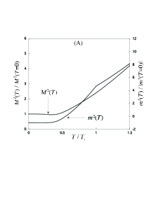
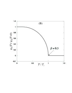
Fig. 2: (A) The tree level mass $M^{2}(T)=m^{2}+\lambda\varphi_{0}/2$, with the left vertical scale and the mass parameter $m^{2}(T)$, with the right vertical scale obtained with the PMS condition. They are normalized by their vales at $T=0$. (B) Vacuum expectation value $\varphi_{0}$ normalized by $\varphi_{0}(T=0)$.

   

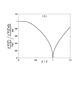
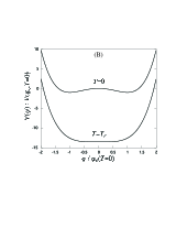
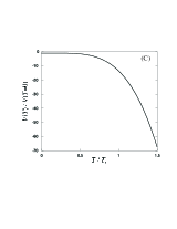
Fig. 3: (A) Second derivative of $V(T)$ with respect to $\varphi$ for the PMS condition. (B) Effective potentials at $T=0$ and $T=T_{c}$. (C) Minimum value of the effective potential as a function of $T$.

3.4 The FAC condition

In this subsection, we apply the FAC condition. The simplest condition to resum the HTLs in this case is

$$\mathchar 28934\relax_{R}(\omega=0,|\vec{k}|=0;T)=0,$$ (3.19)

where $\mathchar 28934\relax_{R}$ is a retarded two-point self-energy which is defined as

$$\mathchar 28934\relax_{R}(\omega,\vec{k};T)=\left.{\partial^{2}V(\varphi,m^{2})\over\partial\varphi^{2}}\right|_{\varphi=\varphi_{0}}.$$ (3.20)

In the following, we investigate the above condition at one-loop and two-loop orders.

3.4.1 1-loop analysis

The HTLs can be resummed even with the one-loop FAC condition of Eq.(3.19). For this reason, this condition has been adopted in many studies for simplicity, and it allows the tachyon problem to be solved at low $T$. However, the phase transition becomes first order with this condition. Here, we do not recapitulate these results, because they are discussed extensively in the literature. Instead, we examine the two-loop condition Eq.(3.19) in §3.4.2 to compare the result with that for the PMS condition discussed in the §3.3.2.

3.4.2 2-loop analysis

Since the physics should not depend on the artificial parameter $m^{2}$, one expects that the result should not depend on the choice of the optimized conditions. However, the 2-loop PMS condition Eq.(3.12) leads to a second-order phase transition, and 1-loop the FAC condition is known to lead to a first-order transition. Therefore, it is necessary to study whether the FAC condition at the two-loop level gives a second order phase transition.

For the FAC condition at $O(\delta^{2})$, we adopt

$$\mathchar 28934\relax_{R}^{\delta^{2}}(\omega,\vec{k};T)=\left.{\partial^{2}V^{\delta^{2}}(\varphi,m^{2})\over\partial\varphi^{2}}\right|_{\varphi=\varphi_{0}}=0.$$ (3.21)

An explicit formula for $V^{\delta^{2}}$ is given in Appendix.B. At high $T$, Eq.(3.21) is reduced to

$$\left.{\partial^{2}V^{\delta^{2}}\over\partial\varphi^{2}}\right|_{\varphi=0} \stackrel{{\scriptstyle\beta m^{2}\rightarrow 0}}{{\longrightarrow}} {\lambda T\over 16\pi m}(\chi-{\lambda T^{2}\over 24})+{\lambda^{2}m^{2}\over 2(4\pi)^{4}}\{c+(-2+{1\over 2}\ln{m^{2}\over\kappa^{2}})\ln{m^{2}\over\kappa^{2}}\}$$ (3.22)

$$+{\lambda^{2}T^{2}\over 24(4\pi)^{2}}(3.30-\ln{T^{2}\over\kappa^{2}}).$$

The first term on the right hand side (r.h.s.) produces the resummation of the HTLs.

Initial conditions

The initial parameters (at $T=0$) are chosen as $\mu^{2}=m^{2}$, $\lambda=10.0$ and $\varphi_{0}=10.0$ as in the previous section. The condition $\mu^{2}=m^{2}$ is needed for agreement with the naive loop-expansion at $T=0$. Note that we recognize that the loop expansion at $T=0$ is a valid approximation. The other resultant values, which are determined by solving Eqs.(3.15) and (3.21) simultaneously, are $\mu^{2}=m^{2}=-166$, $\kappa^{2}=137$ and $M^{2}=m^{2}+{\lambda\over 2}\varphi_{0}^{2}=334$.

Results of the numerical calculation

The results are given in Figs.4 and 5. One can see that the qualitative features of the figures are the same as the PMS results in Figs.2 and 3 . From Fig.4 (A), one can see that the tachyon problem is also avoided in this case. Figures 4 (B), 5 (A) and 5 (B) show the second order phase transition with $\beta=0.5$. In this case, the Gibbs free energy decreases uniformly (Fig.5 (C)). Thus, the 2-loop condition in both PMS and FAC give qualitatively the same results. This is the desired property, and it shows the validity of the OPT.

 

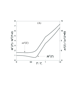
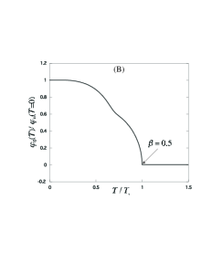
Fig. 4: (A) The tree level mass $M^{2}(T)=m^{2}+\lambda\varphi_{0}/2$, with the left vertical scale, and the mass parameter $m^{2}(T)$, with the right vertical scale, in the case of the FAC condition. They are normalized by their values at $T=0$. (B) Vacuum expectation value $\varphi_{0}$ normalized by $\varphi_{0}(T=0)$.

   

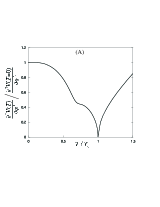
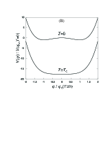
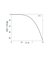
Fig. 5: (A) Second derivative of $V(T)$ with respect to $\varphi$ for the FAC condition. (B) Effective potential at $T=0$ and $T=T_{c}$. (C) Minimum value of the effective potential as a function of $T$.

3.5 Some remarks

We tested the two conditions represented by Eqs.(3.12) and (3.21) in the OPT to study the phase transition for $\lambda\phi^{4}$ theory. The two conditions give qualitatively the same results and show that the resummations were successfully performed. However, there are three remarks in order, which we give below.

FAC with $O(\delta)+O(\delta^{2})$

One may try to use the two-loop FAC condition

$$\mathchar 28934\relax_{R}^{\delta+\delta^{2}}(\omega,\vec{k};T)=\left.{\partial^{2}V^{\delta+\delta^{2}}(\varphi,m^{2})\over\partial\varphi^{2}}\right|_{\varphi=\varphi_{0}}=0$$ (3.23)

instead of Eq.(3.21). This condition implies that all the loop corrections vanish at zero external momentum. In other words, $m^{2}$ contains all contributions up to two-loop order. From Eq.(3.23), the following equation is obtained:

$${\partial^{2}V^{0+\delta+\delta^{2}}\over\partial\varphi^{2}}=M^{2}=m^{2}+{\lambda\over 2}\varphi^{2}.$$ (3.24)

At $T=T_{c}$, if one assumes a second-order phase transition, Eq.(3.24) must be zero; that is $m^{2}(=M^{2})=0$. However, the vanishing of the tree-level mass causes an infrared divergence in the loop integrals. Actually, the left-hand side (l.h.s) of Eq.(3.15) diverges as $M^{2}\rightarrow 0$. Thus, $M^{2}=0$ is never satisfied at $T=T_{c}$. From this argument, we see that a second-order phase transition cannot be realized with the condition given by Eq.(3.24).

Full OPT

The full OPT, which includes an optimization of the coupling constant, allows the possibility not only of avoiding the above infrared problem but also of going beyond the mean field approximation near $T_{c}$. Therefore, it is very interesting to explore it. However, the PMS condition for $V(\varphi,m^{2},g)$ requires tree-loop calculation. This can be understood as follows. Suppose one chooses the PMS condition at the two-loop level as

$${\partial V^{0+\delta+\delta^{2}}(\varphi,m^{2},g)\over\partial m^{2}}=0,\ \ {\partial V^{0+\delta+\delta^{2}}(\varphi,m^{2},g)\over\partial g}=0.$$ (3.25)

In the symmetric phase ($\varphi=0$), Eq.(3.25) can be reduced to

$$\left.{\partial V\over\partial m^{2}}\right|_{\varphi=0} = {\partial K_{t}\over\partial M^{2}}(\chi+gK_{t}),$$ (3.26)

$$\left.{\partial V\over\partial g}\right|_{\varphi=0} = {1\over 2}K_{t}^{2}.$$ (3.27)

From Eq.(3.27), $K_{t}=0$ is obtained. This gives a solution for $m^{2}$. (Note that $K_{t}$ depends on $g$ only through $M^{2}=m^{2}+g\varphi^{2}/2$.) Then, this solution is substituted into Eq.(3.26), giving

$$\left.{\partial V(\varphi,m^{2},g)\over\partial m^{2}}\right|_{\varphi=0}={\partial K_{t}\over\partial M^{2}}\chi=0.$$ (3.28)

Since this relation also does not depend on $g$, we cannot determine $g$. Thus, Eq.(3.25) cannot give a solution for $m^{2}$ and $g$ simultaneously in the symmetric phase.

On the other hand, in the three-loop calculation, $V(\varphi,m^{2},g)$ has the term

$$-g{\partial K_{t}\over\partial M^{2}}(\chi+{g\over 2}K_{t}).$$ (3.29)

This leads to the HTLs (tadpole diagram) in $\partial V/\partial g$, and depends on $g$ even in the symmetric phase. Thus, the full OPT with the PMS condition for the tree-loop effective potential has the possibility of giving a solution for $m^{2}$ and $g$ simultaneously.

What about the FAC condition in full OPT? Suppose we use the following FAC condition:

$${\partial^{2}V^{\delta^{2}}(\varphi,m^{2},g)\over\partial\varphi^{2}}=0,\ \ {\partial^{4}V^{\delta^{2}}(\varphi,m^{2},g)\over\partial\varphi^{4}}=0.$$ (3.30)

Unfortunately, we could not find a solution which improves the previous results near $T_{c}$ at the two-loop level. We have tried all possible variations ($V^{\delta^{2}}(\varphi,m^{2},g)$ in Eq.(3.30) replaced by $V^{\delta+\delta^{2}}(\varphi,m^{2},g)$, $V^{\delta}(\varphi,m^{2},g)$, and so on), but improved solutions were not obtained for the critical exponent. Thus, two-loop order, it seems that it is not possible to improve the previous analysis near $T=T_{c}$ in the full OPT with the FAC condition. In any case, further study along this line is necessary.

Limiting temperature

For sufficiently high $T$, there are no solutions with (3.12) and (3.21) for $m^{2}(T)$, because logarithmic terms of the form $\ln(T/\kappa)$ dominate. This means that the renormalization point $\kappa$, which is fixed at $T=0$, becomes a bad choice as $T$ increases. To avoid this situation, one may try a renormalization group improvement. Since the typical “scale” of this system is $T$, one may choose $\kappa=T$. In this case, no large $\ln(T/\kappa)$ appears. This renormalization group improvement would extend the applicability of OPT. However, in non-asymptotically free theories, such as $\lambda\phi^{4}$ and $O(N)$ $\lambda\phi^{4}$ theories, there eventually appears a Landau pole where the running coupling constant $\lambda(\kappa=T)$ diverges at a certain $T$. [28, 29] Thus, the theory is not applicable beyond this $T$.

4 Summary

In this paper, we have generalized the optimized perturbation theory (OPT) at finite temperature ($T$) in the $\lambda\phi^{4}$ theory to incorporate the optimization of the coupling constant. The naive loop expansion for theories with spontaneous symmetry breaking is known to break down at low $T$ (tachyon pole problem) and high $T$ (hard thermal loops (HTLs) problem). By contrast, we have shown that the OPT does not suffer from such difficulties. This is because that the OPT resums the higher-order terms of the naive perturbation theory in a consistent way by imposing appropriate conditions, such as the principle of minimal sensitivity (PMS) and the fastest apparent convergence (FAC).

The advantages of the OPT over other self-consistent methods are that one can carry out the renormalization of ultraviolet divergences systematically and that the Nambu-Goldstone (NG) theorem at finite $T$ is trivially satisfied at any given order.

In §3, we applied the OPT to $\lambda\phi^{4}$ theory to examine whether it can describe the finite $T$ phase transition correctly. Carrying out the two-loop computation of the effective potential in the OPT, we have found that both PMS and FAC conditions give the correct second order transition. The critical exponent $\beta$, however, is found to coincide with the mean-field value at this level. The full OPT, where both the mass and the coupling constant are shifted, may or may not improve the result. This remains as an open problem.

Application of the idea of the OPT to gauge theories at finite $T$ is also an interesting problem. However, to go beyond the hard thermal loops (HTLs) resummation scheme, one must solve the following two problems.

• Since an infinite number of $N$-point vertex functions ($N$-gauge boson vertices and $(N-2)$-gauge boson 2-fermion vertices) identified with HTLs in gauge theories and a naive mass term breaks the gauge symmetry, one must take into account an infinite number of effective vertices like HTLs resummation scheme. However, this infinite number vertices may create a difficulty for the renormalization.

• It is known that HTLs resummation scheme breaks down at high $T$ due to the so-called magnetic mass problem. [30]

Therefore, we may need further generalization of the OPT to apply it for gauge theories.

A 2-Loop Effective Potential in $\lambda\phi^{4}$-Theory

Here, we calculate the physical effective potential in (2.1) in the real-time formalism, [19] which is equivalent to the effective potential defined in the imaginary-time formalism. Following Ref. [20], we compute the tadpole functions $V^{(1,0)}$, and then the effective potential is integrated over the classical field $\varphi$.[31] Since the propagator in the $T=0$ part and $T\neq 0$ part decouples in the real time formalism, calculations of the $T=0$ parts yield the same results as the ordinary $T=0$ perturbation theory. Hence, we can calculate the $T$-dependent term and $T$-independent term separately.

The Feynman diagrams contributing to the $\varphi_{1}$ tadpole functions up to the two-loop level are shown in Figs.7, 8, 9. The vertex with the number 1 (2) represents the type 1 (2) field self-interaction. The type 2 field is necessary to cancel pathological pinch singularities.

The formulas of the tadpole functions read

$$V^{(1,0)} = V^{(1,0)1}+V^{(1,0)2},$$ (A.1)

$$-iV^{(1,0)1} = -i{\lambda\varphi_{1}\over 2}\kappa^{2\varepsilon}\int{d^{n}k\over(2\pi)^{n}}iD_{\beta}^{11}(k)+counterterms$$ (A.2)

$$V^{(1,0)2} = V^{(1,0)2}_{2bubble}+V^{(1,0)2}_{c}+V^{(1,0)2}_{s},$$ (A.3)

$$-iV^{(1,0)2}_{2bubble} = {(-i\lambda)^{2}\varphi\over 4}\kappa^{4\varepsilon}\left[\int{d^{n}k_{1}\over(2\pi)^{n}}\{iD_{\beta}^{11}(k_{1})\}^{2}\int{d^{n}k_{2}\over(2\pi)^{n}}iD_{\beta}^{11}(k_{2})\right.$$ (A.4)

$$\left.-\int{d^{n}k_{1}\over(2\pi)^{n}}\{iD_{\beta}^{12}(k_{1})\}^{2}\int{d^{n}k_{2}\over(2\pi)^{n}}iD_{\beta}^{22}(k_{2})\right]+counterterms,$$

$$-iV^{(1,0)2}_{c} = -i{\lambda\over 2}(-iB_{1}\mu^{2}-iC_{1}\varphi^{2})\kappa^{2\varepsilon}\int{d^{n}k\over(2\pi)^{n}}\{iD_{\beta}^{11}(k)\}^{2}-\{iD_{\beta}^{12}(k)\}^{2}$$ (A.5)

$$-i{C_{1}\varphi^{2}\over 2}\kappa^{2\varepsilon}\int{d^{n}k\over(2\pi)^{n}}iD_{\beta}^{11}(k),$$

$$-iV^{(1,0)2}_{s} = {(-i\lambda\varphi)^{3}\over 4}\kappa^{6\varepsilon}\int{d^{n}k_{1}\over(2\pi)^{n}}{d^{n}k_{2}\over(2\pi)^{n}}[\{iD_{\beta}^{11}(k_{1})\}^{2}iD_{\beta}^{11}(k_{2})iD_{\beta}^{11}(k_{1}+k_{2})$$ (A.6)

$$-2iD_{\beta}^{11}(k_{1})iD_{\beta}^{12}(k_{1})iD_{\beta}^{12}(k_{2})iD_{\beta}^{12}(k_{1}+k_{2})$$

$$+\{iD_{\beta}^{12}(k_{1})\}^{2}iD_{\beta}^{22}(k_{2})iD_{\beta}^{22}(k_{1}+k_{2})]$$

$$+{(-i\lambda\varphi)(-i\lambda)\over 6}\kappa^{4\varepsilon}\int{d^{n}k_{1}\over(2\pi)^{n}}{d^{n}k_{2}\over(2\pi)^{n}}[iD_{\beta}^{11}(k_{1})iD_{\beta}^{11}(k_{2})iD_{\beta}^{11}(k_{1}+k_{2})$$

$$-iD_{\beta}^{12}(k_{1})iD_{\beta}^{12}(k_{2})iD_{\beta}^{12}(k_{1}+k_{2})]+counterterms,$$

where,

$$iD_{\beta}^{ab}(k) = \left(\begin{array}[]{cc}{i\over k^{2}-\mu^{2}+i\varepsilon}&0\\[8.5359pt] 0&{-i\over k^{2}-\mu^{2}-i\varepsilon}\end{array}\right)$$ (A.12)

$$+2\pi\delta(k^{2}-\mu^{2})\left(\begin{array}[]{cc}{1\over e^{\beta|k_{0}|}-1}&{-e^{-\beta|k_{0}|/2}\over 1-e^{-\beta|k_{0}|}}\\[8.5359pt] {-e^{-\beta|k_{0}|/2}\over 1-e^{-\beta|k_{0}|}}&{1\over e^{\beta|k_{0}|}-1}\end{array}\right),$$

$$M^{2}=\mu^{2}+{\lambda\over 2}\varphi^{2},\ \ \ n_{B}(E)=(e^{\beta E}-1)^{-1},\ \ \ \cosh^{2}\theta={1\over 1-e^{-\beta|k_{0}|}},$$ (A.13)

and $\kappa$ is the renormalization point. The “$(1,0)1$” in $V^{(1,0)1}$ indicates a function which has a one-point type 1 external field and a zero-point type 2 external field at the one-loop level. $-iV^{(1,0)2}_{2bubble}$, $-iV^{(1,0)2}_{c}$ and $-iV^{(1,0)2}_{s}$ are contributed from Figs.8 (a),(b),8 (c)-(e) and Fig.9, respectively.

The above quantities are then integrated over $\varphi$, yielding the following:

$$V^{1} = -{1\over(4\pi)^{2}}{M^{4}\over 4}({3\over 2}-\ln{M^{2}\over\kappa^{2}})+\int^{\infty}_{0}{dk\over(2\pi)^{2}}{2\over\beta}k^{2}\ln(1-e^{-\beta E}),$$ (A.14)

$$V^{2}_{2bubble} = {\lambda\over 2}K_{t}^{2}-{\lambda M^{2}\over 4}C_{f},$$ (A.15)

$$V^{2}_{c} = {\lambda\over 4}(\mu^{2}+{3\over 2}\lambda\varphi^{2})C_{f},$$ (A.16)

$$V^{2}_{s} = {\lambda^{2}\varphi^{2}\over 4}\left[{M^{2}\over(4\pi)^{4}}\{a+(\gamma-\ln{4\pi}-3+\ln{M^{2}\over\kappa^{2}})\ln{M^{2}\over\kappa^{2}}\}\right.$$ (A.17)

$$\left.+{1\over 2(2\pi)^{2}}(\ln{M^{2}\over\kappa^{2}}-2+{\pi\over\sqrt{3}})I_{t}+I_{l}\right]$$

$$\equiv {\lambda^{2}\varphi^{2}\over 4}S_{s},$$

where,

$$E = \sqrt{k^{2}+M^{2}},$$ (A.18)

$$K_{t} = {M^{2}\over 2(4\pi)^{2}}(1-\ln{M^{2}\over\kappa^{2}})-I_{t}$$ (A.19)

$$C_{f} = {M^{2}\over(4\pi)^{4}}\{d-(\gamma-\ln 4\pi-1+{1\over 2}\ln{M^{2}\over\kappa^{2}})\ln{M^{2}\over\kappa^{2}}\},$$ (A.20)

$$d = -{1\over 2}(\gamma^{2}-2\gamma+2+{\pi^{2}\over 6})+(\gamma-1-{1\over 2}\ln 4\pi)\ln 4\pi\simeq-5.68496,$$ (A.21)

$$a = {\pi^{2}\over 12}+{9\over 2}+{1\over 2}(\gamma-\ln 4\pi)(\gamma-\ln 4\pi-3)$$ (A.22)

$$+\int^{1}_{0}dx\int^{1}_{o}dy-\ln y(\ln\alpha-{(1-y)\beta\over\alpha})$$

$$\simeq 10.16186-2.17195=7.98891,$$

$$\alpha = -(y-1+{y\over x^{2}-x}),\ \ \beta=-(1+{1\over x^{2}-x}),$$ (A.23)

$$I_{t} = \int^{\infty}_{0}{dk\over(2\pi)^{2}}{k^{2}n_{B}(E)\over E},$$ (A.24)

$$I_{l} = \int^{\infty}_{0}{dk_{1}dk_{2}\over(2\pi)^{4}}{k_{1}k_{2}n_{B}(E_{1})n_{B}(E_{2})\over 2E_{1}E_{2}}\ln\left|{4E_{1}^{2}E_{2}^{2}-(M^{2}+2k_{1}k_{2})^{2}\over 4E_{1}^{2}E_{2}^{2}-(M^{2}-2k_{1}k_{2})^{2}}\right|,$$ (A.25)

and $\gamma$ is the Euler constant.

Fig. 6: One-loop effective potential diagrams.

Fig. 7: (a) One-loop diagram contributing to the 1-point function. (b) Counterterm contribution (which includes all $\hbar$-order contributions in principle). The index 1 indicates a type 1 vertex. The cross represents the counterterms.

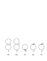
Fig. 8: (a) and (b) 2-bubble diagrams. (c)-(e) Tadpole diagrams including counterterms.

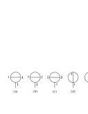
Fig. 9: Diagrams which contribute to the setting sun diagram.

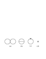
Fig. 10: Two-loop effective potential diagrams.

B OPT Equations

Here, we summarize the calculations of the effective potential and its derivatives in the full OPT.

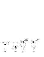
Fig. 11: (a) Additional $O(\delta)$ contributions to the 1-point function in the full OPT. (b)-(d) Additional $O(\delta^{2})$ contributions to the 1-point function.

Fig. 12: (a) Additional $O(\delta)$ contributions to the effective potential in the full OPT. (b) Additional $O(\delta^{2})$ contributions.

The two-loop effective potential in the full optimized perturbation theory reads

$$V = V^{0}+V^{\delta}+V^{\delta^{2}},$$ (B.1)

$$V^{0} = {1\over 2}m^{2}\varphi^{2}+{g\over 4!}\varphi^{4},$$ (B.2)

$$V^{\delta} = -{1\over 2}\chi\varphi^{2}-{\eta\over 4!}\varphi^{4}-{1\over(4\pi)^{2}}{M^{4}\over 4}({3\over 2}-\ln{M^{2}\over\kappa^{2}})$$ (B.3)

$$+\int^{\infty}_{0}{dk\over(2\pi)^{2}}{2\over\beta}k^{2}\ln(1-e^{-\beta E}),$$

$$V^{\delta^{2}} = (\chi+{\eta\varphi^{2}\over 2}+{g\over 2}K_{t})K_{t}+{g^{2}\varphi^{2}\over 4}T_{f},$$ (B.4)

where,

$$\begin{array}[]{lcccl}\mu^{2}&=&m^{2}-(m^{2}-\mu^{2})&=&m^{2}-\chi,\\ \lambda&=&g-(g-\lambda)&=&g-\eta,\end{array}$$ (B.7)

$$K_{t} = {M^{2}\over 2(4\pi)^{2}}(1-\ln{M^{2}\over\kappa^{2}})-I_{t},$$ (B.8)

$$T_{f} \equiv S_{s}+C_{f}$$ (B.9)

$$= {M^{2}\over(4\pi)^{4}}\{c+(-2+{1\over 2}\ln{M^{2}\over\kappa^{2}})\ln{M^{2}\over\kappa^{2}}\}$$

$$+{1\over 2(2\pi)^{2}}(\ln{M^{2}\over\kappa^{2}}-2+{\pi\over\sqrt{3}})I_{t}+I_{l},$$

$$I_{t} = \int^{\infty}_{0}{dk\over(2\pi)^{2}}{k^{2}n_{B}(E)\over E},$$ (B.10)

$$I_{l} = \int^{\infty}_{0}{dk_{1}dk_{2}\over(2\pi)^{4}}{k_{1}k_{2}n_{B}(E_{1})n_{B}(E_{2})\over 2E_{1}E_{2}}\ln\left|{4E_{1}^{2}E_{2}^{2}-(M^{2}+2k_{1}k_{2})^{2}\over 4E_{1}^{2}E_{2}^{2}-(M^{2}-2k_{1}k_{2})^{2}}\right|,$$ (B.11)

$$M^{2}=m^{2}+{g\over 2}\varphi^{2},\ \ E=\sqrt{k^{2}+M^{2}},\ \ n_{B}(E)=(e^{\beta E}-1)^{-1},$$ (B.12)

$$c = {1\over 2}(7-\gamma+\ln 4\pi)-\int^{1}_{0}dx\int^{1}_{0}dy\ln y(\ln\alpha-{(1-y)\beta\over\alpha})$$ (B.13)

$$\simeq 2.30495,$$

$$\alpha = -(y-1+{y\over x^{2}-x}),\ \ \beta=-(1+{1\over x^{2}-x}),$$ (B.14)

and $\gamma=0.5772\cdots$.

B.1 For PMS conditions

Here, we give equations needed to study the PMS conditions. In the following, we set $g=\lambda$, so $\eta=0$ in Eq.(B.1):

$${\partial V\over\partial\varphi} = {\partial V^{0}\over\partial\varphi}+{\partial V^{\delta}\over\partial\varphi}+{\partial V^{\delta^{2}}\over\partial\varphi},$$ (B.15)

$${\partial V^{0}\over\partial\varphi} = \varphi\left[m^{2}+{\lambda\over 6}\varphi^{2}\right],$$ (B.16)

$${\partial V^{\delta}\over\partial\varphi} = \varphi\left[-\chi-\lambda K_{t}\right],$$ (B.17)

$${\partial V^{\delta^{2}}\over\partial\varphi} = \varphi\left[\lambda(\chi+\lambda K_{t}){\partial K_{t}\over\partial M^{2}}+{\lambda^{2}\over 2}(T_{f}+{\lambda\varphi^{2}\over 2}{\partial T_{f}\over\partial M^{2}})\right].$$ (B.18)

The partial derivative with respect to $m^{2}$ is found to be

$${\partial V\over\partial m^{2}} = {\partial V^{0}\over\partial m^{2}}+{\partial V^{\delta}\over\partial m^{2}}+{\partial V^{\delta^{2}}\over\partial m^{2}},$$ (B.19)

$${\partial V^{0}\over\partial m^{2}} = {1\over 2}\varphi^{2},$$ (B.20)

$${\partial V^{\delta}\over\partial m^{2}} = -K_{t}-{1\over 2}\varphi^{2},$$ (B.21)

$${\partial V^{\delta^{2}}\over\partial m^{2}} = K_{t}+(\chi+\lambda K_{t}){\partial K_{t}\over\partial M^{2}}+{\lambda^{2}\varphi^{2}\over 4}{\partial T_{f}\over\partial M^{2}}.$$ (B.22)

Also, when $\varphi=0$, (B.19) read

$$\left.{\partial V\over\partial m^{2}}\right|_{\varphi=0}=(\chi+\lambda K_{t}){\partial K_{t}\over\partial M^{2}}.$$ (B.23)

B.2 For FAC conditions

The second derivative of the effective potential with respect to $\varphi$ for the FAC conditions is found to be

$${\partial^{2}V\over\partial\varphi^{2}} = {\partial^{2}V^{0}\over\partial\varphi^{2}}+{\partial^{2}V^{\delta}\over\partial\varphi^{2}}+{\partial^{2}V^{\delta^{2}}\over\partial\varphi^{2}},$$ (B.24)

$${\partial^{2}V^{0}\over\partial\varphi^{2}} = m^{2}+{\lambda\over 2}\varphi^{2},$$ (B.25)

$${\partial^{2}V^{\delta}\over\partial\varphi^{2}} = -\chi-\lambda K_{t}-\lambda^{2}\varphi^{2}{\partial K_{t}\over\partial M^{2}},$$ (B.26)

$${\partial^{2}V^{\delta^{2}}\over\partial\varphi^{2}} = \lambda{\partial K_{t}\over\partial M^{2}}(\chi+\lambda K_{t}+\lambda^{2}\varphi^{2}{\partial K_{t}\over\partial M^{2}})+\lambda^{2}\varphi^{2}{\partial^{2}K_{t}\over\partial(M^{2})^{2}}(\chi+\lambda K_{t})$$ (B.27)

$$+{\lambda^{2}\over 2}(T_{f}+{5\over 2}\lambda\varphi^{2}{\partial T_{f}\over\partial M^{2}}+{1\over 2}\lambda^{2}\varphi^{4}{\partial^{2}T_{f}\over\partial(M^{2})^{2}}).$$

B.3 High $T$ forms

Here, we give the high $T$ ($\beta M\rightarrow 0$) forms of Eq.(B.8), derivatives of Eq.(B.8) and Eq.(B.11). We find

$$K_{t} \rightarrow -{T^{2}\over 24}+{MT\over 8\pi}+{M^{2}\over 2(4\pi)^{2}}(1-\ln{T^{2}\over\kappa^{2}})-{M^{2}\over(4\pi)^{2}}(\ln 4\pi-\gamma+{1\over 2}),\hskip 11.38092pt$$ (B.28)

$${\partial K_{t}\over\partial M^{2}} \rightarrow {T\over 16\pi M}+{1\over 2(4\pi)^{2}}(1-\ln{T^{2}\over\kappa^{2}})-{1\over(4\pi)^{2}}(\ln 4\pi-\gamma+{1\over 2}),$$ (B.29)

$${\partial^{2}K_{t}\over\partial(M^{2})^{2}} \rightarrow -{T\over 32\pi M^{3}},$$ (B.30)

$$I_{l} \rightarrow {T^{2}\over 12(4\pi)^{2}}(\ln{M^{2}\over T^{2}}+3.48871).$$ (B.31)

References

- [1]
- [2] Quark Matter ’99, Nucl. Phys. A661 (1999).
- [3] LATTICE ’98, Nucl. Phys. B (Proc. Suppl.) 73 (1999).
- [4] A. Ukawa, Nucl. Phys. B (Proc. Suppl.) 53 (1997), 106.
- [5] A possible way to extract the real-time dynamics has been recently studied in Y. Nakahara, M. Asakawa and T. Hatsuda, Phys. Rev. D60 (1999), 091503.
-
[6]
E. Braaten and R. D. Pisarski, Nucl. Phys. B337 (1990),
569 ; B339 (1990), 310.
J. Frenkel and J. C. Taylor, Nucl. Phys. B334 (1990), 199;
B374 (1992), 156.
J. C. Taylor and S. M. H. Wong, Nucl. Phys. B346 (1990), 115. -
[7]
S. Weinberg, Phys. Rev. D9 (1974), 3357.
L. Dolan and R. Jackiw, Phys. Rev. D9 (1974), 3320. - [8] D. A. Kirzhnits and A. D. Linde, Ann. of Phys. 101 (1976), 195.
-
[9]
E. Braaten, R. D. Pisarski and T. C. Yuan,
Phys. Rev. Lett. 64 (1990), 2242.
S. M. H. Wong, Z. Phys. C53 (1992), 465. E. Braaten and R. D. Pisarski, Phys. Rev. Lett. 64 (1990), 1338; Phys. Rev. D42 (1990), 2156; D46 (1992), 1829. R. Kobes, G. Kunstatter and K. W. Mak, Phys. Rev. D54 (1992), 4632. -
[10]
H. Nakkagawa and H. Yokota, Mod. Phys. Lett. A11 (1996),
2259; hep-ph/9811469 (1998).
K. Ogure and J. Sato, Phys. Rev. D58 (1998), 085010.
Y. Nemoto, K. Naito and M. Oka, hep-ph/9911431 (1999) and references therein. -
[11]
G. Baym and G. Grinstein, Phys. Rev. D15 (1977), 2897.
D. A. Kirzhnits and A. D. Linde, Ann. of Phys. 101 (1976), 195. H. E. Haber and H. A. Weldon, Phys. Rev. D25 (1982), 502.
G. Amelino-Camelia and S-Y. Pi, Phys. Rev. D47 (1993), 2356. G. Amelino-Camelia, Nucl. Phys. B476 (1996), 255; Phys. Lett. B407 (1997), 268.
H-S. Roh and T. Matsui, Eur. Phys. J. A1 (1998), 205.
See also, Y. Nemoto, K. Naito and M. Oka, hep-ph/9911431 (1999). - [12] S. Chiku and T. Hatsuda, Phys. Rev. D57 (1998), R6; D58 (1998), 076001.
-
[13]
A. Okopińska, Phys. Rev. D36 (1987), 2415;
Mod. Phys. Lett. A12 (1997), 1003.
See also, G. A. Hajj and P. M. Stevenson, Phys. Rev. D37 (1988), 413. - [14] N. Banerjee and S. Mallik, Phys. Rev. D43 (1991), 3368.
- [15] P. M. Stevenson, Phys. Rev. D23 (1981), 2916.
- [16] W. A. Bardeen, A. J. Buras, D. W. Duke and T. Muta, Phys. Rev. D18 (1978), 3998.
-
[17]
R. Jackiw, Phys. Rev. D9 (1974), 1686.
See e.g., J. Negele and H. Orland, Quantum Many-Particle Systems (Addison-Wesley, New York, 1988). -
[18]
R. E. Norton and J. M. Cornwall, Ann. of Phys. 91 (1975),
106.
M. B. Kislinger and P. D. Morley, Phys. Rev. D13 (1976), 2771.
H. Matsumoto, I. Ojima and H. Umezawa, Ann. Phys. 152 (1984), 348. -
[19]
Y. Takahashi and H. Umezawa, Collective Phenom. 2
(1975), 55.
N. P. Landsman and Ch. G. van Weert, Phys. Rep. 145
(1987), 143. M. Le Bellac, Thermal Field Theory, (Cambridge Univ. Press, Cambridge, 1996). - [20] A. J. Niemi and G. W. Semenoff, Ann. of Phys. 152 (1984), 105; Nucl. Phys. B230 [FS10] (1984), 181.
- [21] See e.g., P. Ramond, FIELD THEORY:A MODERN PRIMER 2nd ed. (Addison-Wesley, New York, 1990).
-
[22]
C. Ford and D. R. T. Jones, Phys. Lett. B274 (1992), 409
and references therein. See, also 3-loop case,
J. -M. Chung and B. K. Chung, Phys. Rev. D56 (1997), 6508.
J.Korean Phys.Soc. 33 (1998), 634. -
[23]
R. R. Parwani Phys. Rev. D45, (1992) 4695; erratum,
D48, (1993) 5965.
See also, F. Karsch, A. Patkos and P. Petreczky, Phys. Lett. B401, 69 (1997). - [24] P. Arnold and O. Espinosa, Phys. Rev. D47 (1993) 3546.
-
[25]
K. G. Wilson and J. Kogut, Phys. Rep. 12C (1974) 75.
See e.g. N. Goldenfeld, Lectures on Phase Transitions and the Renormalization Group, (Addison-Wesley, New York, 1992). -
[26]
H. W. J. Blöte, A. Compagner, J. H. Croockewit,
Y. T. J. C. Fonk, J. R. Heringa, A. Hoogland, T. S. Smit and
A. L. van Villingen, Physica A161 (1989) 1.
K. Kanaya and S. Kaya, Phys. Rev. D51 (1995), 2404 and references therein. - [27] S. Mallik and K. Mukherjee, hep-th/9607087 (1996).
- [28] W. A. Bardeen and M. Mosche, Phys. Rev. D28 (1983), 1372.
- [29] M. Lüscher and P. Weisz, Nucl. Phys. B290 [FS20] (1987), 25; B290 [FS21] (1988), 65; ibid. B318 (1989), 705.
-
[30]
A. D. Linde, Phys. Lett. 96B (1980), 289.
See also, T. Hatsuda, Phys. Rev. D56 (1997), 8111 and references therein. - [31] S. Weinberg, Phys. Rev. D7 (1973), 2887.