SLAC–PUB–8711
November 2000
revised April 2001

Abstract

The light-front (LF) quantization of QCD in light-cone gauge has a number of remarkable advantages, including explicit unitarity, a physical Fock expansion, the absence of ghost degrees of freedom, and the decoupling properties needed to prove factorization theorems in high momentum transfer inclusive and exclusive reactions. We present a systematic study of LF-quantized gauge theory following the Dirac method and construct the Dyson-Wick S-matrix expansion based on LF-time-ordered products. The free theory gauge field is shown to satisfy the Lorentz condition as an operator equation as well as the light-cone gauge condition. Its propagator is found to be transverse with respect to both its four-momentum and the gauge direction. The interaction Hamiltonian of QCD can be expressed in a form resembling that of covariant theory, except for additional instantaneous interactions which can be treated systematically. The renormalization constants in YM theory are shown to satisfy the identity $Z_{1}=Z_{3}$ at one loop order. The QCD $\beta$ function computed in the noncovariant light-cone gauge agrees with that known in the conventional framework. Some comments on the relationship of our LF framework, with the doubly transverse gauge propagator, to the analytic effective charge and renormalization scheme defined by the pinch technique, the unitarity relations and the spectral representation are also made. LF quantization thus provides a consistent formulation of gauge theory, despite the fact that the hyperplanes $x^{\pm}=0$ used to impose boundary conditions constitute characteristic surfaces of a hyperbolic partial differential equation.

to appear in Physical Review D15, July 2001

Keywords: Quantum Chromodynamics; Quantization; Light-cone gauge; Light-front; Constraints; Gauge Theory; Propagator

1 Introduction

The quantization of relativistic field theory at fixed light-front time $\tau=(t-z/c)/\sqrt{2}$, which was proposed by Dirac [1] half a century ago, has found important applications [2, 3, 4, 5] in both gauge theory and string theory [6]. The light-front (LF) quantization of QCD in its Hamiltonian form provides an alternative to lattice gauge theory for the computation of nonperturbative quantities such as the spectrum and the light-front Fock state wavefunctions of relativistic bound states [3]. LF variables have also found natural applications in other contexts, such as in the quantization of (super-) string theory and M-theory [6]. Light-front quantization has been employed in the nonabelian bosonization [7] of the field theory of $N$ free Majorana fermions and was used in the demonstration of the asymptotic freedom of the Yang-Mills theory beta-function [8]. The requirement of the microcausality[9] implies that the LF framework is more appropriate for quantizing [10] the self-dual (chiral boson) scalar field.

Since LF coordinates are not related to the conventional coordinates by a finite Lorentz transformation, the descriptions of the same physical result may be different in the equal-time (instant form) and equal-LF-time (front form) formulations of the theory. This was in fact found to be the case in a recent study [11, 12] of some soluble two-dimensional gauge theory models, where it was also demonstrated that LF quantization is very economical in displaying the relevant degrees of freedom, leading directly to a physical Hilbert space. The corresponding Fock representation is boost independent since the front form has seven kinematical Poincaré generators [1], including Lorentz boost transformations, compared to only six in the instant form framework. LF-time-ordered perturbation theory is much more economical than equal-time-ordered perturbation theory, since only graphs with particles with positive LF momenta $p^{+}=(p^{0}+p^{3})/\sqrt{2}$ appear. LF-time-ordered perturbation theory has also been applied [13, 14] to massive fields. It was used in the analysis of the evolution of deep inelastic structure functions [15] and the evolution of the distribution amplitudes which control hard exclusive processes in QCD [16]. Recently, light-cone gauge on the light-front has been used to analyze the forces between fixed colored sources [18], the string structure of QCD at large $N_{C}$ [17], and spontaneous symmetry breaking phenomena without zero modes [19]. There have also been interesting applications to supersymmetric theories on the light-front [20].

It has been conventional to apply LF quantization to gauge theory in light-cone (l.c.) gauge $A^{+}=A_{-}=(A^{0}+A^{3})/\sqrt{2}=0$, since the transverse degrees of freedom of the gauge field can be immediately identified as the dynamical degrees of freedom, and ghost fields can be ignored in the quantum action of the nonabelian gauge theory [16, 21, 22]. The light-front (LF) quantization of quantum chromodynamics in l.c. gauge thus has a number of remarkable advantages, including explicit unitarity, a physical Fock expansion, and the complete absence of ghost degrees of freedom. In addition, the decoupling of gluons to propagators carrying high momenta and the absence of collinear divergences in irreducible diagrams in the l.c. gauge are important tools for proving the leading-twist factorization of soft and hard gluonic corrections in high momentum transfer inclusive and exclusive reactions [16]. On the negative side, any noncovariant gauge brings in the breaking of manifest rotational invariance, instantaneous interactions, and, apparently, a more difficult renormalization procedure [21, 22, 23].

In this paper we will discuss the LF quantization of QCD gauge field theory in l.c. gauge employing the Dyson-Wick S-matrix expansion [24] based on LF-time-ordered products [25]. We shall first study the gauge-fixed quantum action of the theory on the LF. The LF Hamiltonian framework will then be constructed following the Dirac method [26, 27] which allows one to self-consistently identify the independent fields and their commutation relations in the presence of the l.c. gauge condition and other constraints. It also allows us to study [26] the Lorentz covariance properties of the theory.

The LF framework is a severely constrained dynamical theory with many second-class constraints. These can be eliminated by constructing Dirac brackets, and the theory can be quantized canonically by the correspondence principle in terms of a reduced number of independent fields. The commutation relations among the field operators are also found by the Dirac method, and they are used to obtain the momentum space expansions of the fields. For example, the nondynamical projection of the fermion field can be eliminated using a nonlocal constraint equation. The gauge-field quantization of the massless field in the l.c. gauge in the front form theory is studied. Using the derived commutators, we find that LF quantized free gauge theory simultaneously satisfies the covariant gauge condition $\partial\cdot A=0$ as an operator condition as well as the light-cone gauge condition. The Fourier transform of the free theory gauge field and its propagator in momentum space then follow straightforwardly. The removal of the unphysical components of the fields results in [2, 28] tree-level instantaneous interaction terms which can be evaluated systematically (See Sections 4 and 5). The instantaneous light-cone gauge interactions of the light-front Hamiltonian are incorporated into nonperturbative approaches such as DLCQ [29].

The QCD interaction Hamiltonian is constructed in Section 4 where we restore in the expression the dependent components $A_{+}$ and $\psi_{-}$. It then takes a form close to that of covariant gauge theory without ghost terms, plus instantaneous interactions which are straightforward to handle in the Dyson-Wick perturbation theory.

The renormalization procedure in our framework is illustrated in Section 5 by considering the nonabelian YM gauge theory. The equality $Z_{1}=Z_{3}$ is explicitly demonstrated to one loop in our doubly transverse gauge framework and the $\beta-$function is found to agree with that known in the conventional Feynman gauge calculation. The results are compared with those found [21, 22, 30] in the conventional l.c. gauge equal-time framework. Gluon self-energy coming from quark loops is also computed. A calculation of the electron-muon scattering amplitude in QED is used to show the relevance of instantaneous interactions for recovering the Lorentz invariance. We recall that the Dyson-Wick expansion has been used [31] to renormalize two-dimensional scalar field theory on the LF with nonlocal interactions. Appendix C comments on the understanding in the gluon self-energy of a noncovariant $\log$ term, which arises from another basic noncovariant divergent integral, present in the noncovariant gauge under study. Its relevance in the context of the spectral representation and unitarity is briefly touched upon. The complete renormalization of QCD in our framework, including the verification of Slavnov-Taylor identities, will be considered in a forthcoming paper.

2 QCD Action in Light-Cone Gauge

The LF coordinates are defined as $x^{\mu}=(x^{+}=x_{-}=(x^{0}+x^{3})/{\sqrt{2}},\,x^{-}=x_{+}=(x^{0}-x^{3})/{\sqrt{2}},\,x^{\perp})$, where $x^{\perp}=(x^{1},x^{2})=(-x_{1},-x_{2})$ are the transverse coordinates and $\,\mu=-,+,1,2$. The coordinate $x^{+}\equiv\tau$ will be taken as the LF time, while $x^{-}$ is the longitudinal spatial coordinate. We can of course choose a convention where the role of $x^{+}$ and $x^{-}$ interchanged. The equal-$x^{+}$ quantized theory already contains the information on the equal-$x^{-}$ commutator [11, 12]. The LF components of any tensor, for example, the gauge field, are similarly defined, and the metric tensor $g_{{\mu}{\nu}}$ may be read from $A^{\mu}B_{\mu}=A^{+}B^{-}+A^{-}B^{+}-A^{\perp}B^{\perp}$. Also $k^{+}$ indicates the longitudinal momentum, while $k^{-}$is the corresponding LF energy.

The quantum action of QCD in l.c. gauge is described in standard notation by the following Lagrangian density

$${\cal L}_{QCD}=-{1\over 4}F^{a\mu\nu}{F^{a}}_{\mu\nu}+B^{a}{A^{a}}_{-}+{\bar{c}}^{a}{\cal D}^{ab}_{-}c^{b}+{\bar{\psi}}^{i}(i\gamma^{\mu}{D^{ij}}_{\mu}-m\delta^{ij})\psi^{j}$$ (1)

Here $\psi^{j}$ is the quark field with color index $j=1..N_{c}$ for an $SU(N_{c})$ color group, ${A^{a}}_{\mu}$ the gluon field, $F^{a}_{\mu\nu}=\partial_{\mu}A^{a}_{\nu}-\partial_{\nu}{A^{a}}_{\mu}+gf^{abc}{A^{b}}_{\mu}{A^{c}}_{\nu}$ the field strength, ${{\cal D}^{ac}}_{\mu}=(\delta^{ac}\partial_{\mu}+gf^{abc}{A^{b}}_{\mu})$, ${D^{ij}}_{\mu}\psi^{j}=(\delta^{ij}\partial_{\mu}-ig{A^{a}}_{\mu}{t^{a}}^{ij})\psi^{j}$, $t^{a}\equiv\lambda^{a}/2$, $a=1..({N_{c}}^{2}-1)$, the gauge group index, and $\,{\bar{c}}^{a},c^{a}$ are anti-commuting ghost fields. In writing the quantum action we introduce auxiliary Lagrange multiplier fields $B^{a}(x)$ and add to the Lagrangian the linear gauge-fixing term $(B^{a}{A^{a}}_{-})$, which is a traditional procedure. In addition we are required to also add ghost terms such that the action (1) becomes invariant under BRS symmetry [32] transformations.

It is worth recalling the corresponding procedure for implementing a covariant gauge-fixing condition. For example, in Feynman gauge one adds the term $(B^{a}\partial^{\mu}A_{a\mu}+B^{a}B^{a}/2)$ to the Lagrangian. The quadratic $B^{a}B^{a}$ term is allowed on dimensional considerations. However in the case of l.c. gauge, the auxiliary field $B^{a}$ carries canonical dimension three and as such a quadratic term is not allowed in (1). We mention yet another example: the quantum action for constructing [10] the quantized theory of the self-dual scalar field (chiral boson) in two-dimensional space-time. One starts by adding the traditional linear term $B\partial_{-}\phi$ to the free scalar field Lagrangian. Its LF quantization can be performed without any violation of the principle of microcausality, in contrast to that occurs in the conventional treatment. The quantized theory is found to be trivial indicating that the traditional Lagrange multiplier method breaks down at the quantum level. However, if we add to the theory an additional $B^{2}$ term, which is allowed on dimensional considerations, the LF quantization of the improved theory does produce a satisfactory description [10] of the quantized left- and right-movers. The theory also contains as a special case the well known Floreanini-Jackiw action [33], giving a plausible reason for the success of that model.

The quark field term in LF coordinates reads in the notation of Appendix B as

$${\bar{\psi}}^{i}(i\gamma^{\mu}{D^{ij}}_{\mu}-m\delta^{ij})\psi^{j} = i{\sqrt{2}}{\bar{\psi}_{+}}^{i}\gamma^{0}{D^{ij}}_{+}{\psi_{+}}^{j}+{\bar{\psi}_{+}}^{i}(i\gamma^{\perp}{D^{ij}}_{\perp}-m\delta^{ij}){\psi_{-}}^{j}$$ (2)

$$+ {\bar{\psi}_{-}}^{i}\left[{i\sqrt{2}}\gamma^{0}{D^{ij}}_{-}{\psi_{-}}^{j}+(i\gamma^{\perp}{D^{ij}}_{\perp}-m\delta^{ij}){\psi_{+}}^{j}\right]$$

This shows that the minus components ${\psi_{-}}^{j}$ are in fact nondynamical (Lagrange multiplier) fields without kinetic terms. The variation of the action with respect to ${{\bar{\psi^{j}}}_{-}}$ and ${{{\psi^{j}}}_{-}}$ leads to the following gauge-covariant constraint equation

$$i{\sqrt{2}}\,\,{D^{ij}}_{-}{\psi_{-}}^{j}=-(i\gamma^{0}\gamma^{\perp}{D^{ij}}_{\perp}-m\gamma^{0}\delta^{ij}){\psi_{+}}^{j},$$ (3)

and its conjugate. The ${\psi^{j}}_{-}$ components may thus be eliminated in favor of the independent dynamical component $\psi_{+}^{j}$. It gives rise to instantaneous terms in the interaction Hamiltonian given in Sec 4 and also the free theory propagator of $\psi_{+}$ is found [28] to be causal and carries no instantaneous term.

3 Gauge Field Propagator in l.c. Gauge

The quadratic terms in the Lagrangian density which determine the free gauge field propagators are

$$\frac{1}{2}\left[{F^{a}}_{+-}{F^{a}}_{+-}+2{F^{a}}_{+{\perp}}{F^{a}}_{-{\perp}}-{F^{a}}_{12}{F^{a}}_{12}\right]+B^{a}{A^{a}}_{-}+{\bar{c}}^{a}\partial_{-}c^{a}.$$ (4)

We observe that in the front form framework, the fields ${A^{a}}_{+}$ as well as $B^{a}$ have no kinetic terms, and they enter in the action as auxiliary multiplier fields. Also, since the ghost fields decouple, it is sufficient to study the free abelian gauge theory with the following action

$$\int d^{2}x^{\perp}dx^{-}\left\{{1\over 2}\left[(F_{+-})^{2}-(F_{12})^{2}+2F_{+\perp}F_{-\perp}\right]+BA_{-}\right\}$$ (5)

where $F_{\mu\nu}$ stands for $(\partial_{\mu}A_{\nu}-\partial_{\nu}A_{\mu})$ in the present section. The gauge field equations of motion are $\,\framebox{\rule[2.5892pt]{0.0pt}{2.5892pt}\,\ }A_{\mu}=\partial_{\mu}(\partial\cdot A)-B{\delta_{\mu}}^{-}$, $A_{-}=0$, $\mu=-,+,\perp\,$ and $\perp=1,2$, and as a consequence $\partial_{-}B=0$. The canonical momenta following from (5) are $\pi^{+}=0$, $\pi_{B}=0$, $\pi^{\perp}=F_{-\perp}$, and $\pi^{-}=F_{+-}=(\partial_{+}A_{-}-\partial_{-}A_{+})\,$ which indicates that we are dealing with a constrained dynamical system. The Dirac procedure will be followed in order to construct the self-consistent Hamiltonian theory which is required for performing canonical quantization. The canonical Hamiltonian density is

$${\cal H}_{c}={1\over 2}({\pi}^{-})^{2}+{1\over 2}(F_{12})^{2}-A_{+}(\partial_{-}\pi^{-}+\partial_{\perp}\pi^{\perp})-BA_{-}$$ (6)

The primary constraints following from (5) are $\pi^{+}\approx 0$, $\,\pi_{B}\approx 0$ and $\,{\eta^{\perp}}\equiv\pi^{\perp}-\partial_{-}A_{\perp}+\partial_{\perp}A_{-}\approx 0$, where $\,\approx\,$ stands for the weak equality relation. We now require the persistency in $\tau$ of these constraints employing the preliminary Hamiltonian, which is obtained by adding to the canonical Hamiltonian the primary constraints multiplied by the undetermined Lagrange multiplier fields $u_{+}$, $u_{\perp}$, and $u_{B}$. In order to obtain the Hamilton’s equations of motion, we assume initially the standard Poisson brackets for all the dynamical variables present in (6).

We are then led to the following secondary constraints

$$\Phi\equiv\partial_{-}\pi^{-}+\partial_{\perp}\pi^{\perp} \approx 0,$$

$$A_{-} \approx 0$$ (7)

which are already present in (6) multiplied by Lagrange multiplier fields. Requiring also the persistency of $\Phi$ and $A_{-}$ leads to another secondary constraint

$$\Psi\equiv\pi^{-}+\partial_{-}A_{+}\approx 0.\$$ (8)

The procedure stops at this stage, and no more constraints are seen to arise since further repetition leads to equations which would merely determine the multiplier fields.

Let us now analyze the nature of the phase space constraints. In spite of the gauge-fixing term introduced in the initial Lagrangian, there still remains on the canonical LF phase space a first class constraint $\pi_{B}\approx 0$. An inspection of the equations of motion shows that we may add [26] to the set of constraints found above an additional external constraint $B\approx 0$. This would make the whole set of constraints in the theory second class. Dirac brackets satisfy the property such that we can set the above set of constraints as strong equality relations inside them. The equal-$\tau$ Dirac bracket $\{f(x),g(y)\}_{D}$ which carries this property is straightforward to construct. Hamilton’s equations now employ the Dirac brackets rather than the Poisson ones. The phase space constraints on the light front: $\pi^{+}=0$, $\eta^{\perp}=0$, $A_{-}=0$, $\Phi=0$, $\Psi=0$, $\pi_{B}=0$, and $B=0$ thus effectively eliminate $B$ and all the canonical momenta from the theory. The surviving dynamical variables are $A_{\perp}$ while $A_{+}$ is a dependent variable which satisfies $\partial_{-}(\partial_{-}A_{+}-\partial_{\perp}A_{\perp})=0$. The reduced Hamiltonian is found to be

$${H_{0}}^{LF}={1\over 2}\int{d^{2}x^{\perp}}dx^{-}\;\left[(\partial_{-}A_{+})^{2}+\frac{1}{2}F_{\perp\perp^{\prime}}F^{\perp\perp^{\prime}}\right],$$ (9)

where we have retained the dependent variable $A_{+}$ for convenience.

The canonical quantization of the theory at equal-$\tau$ is performed via the correspondence $i\{f(x),g(y)\}_{D}\to\left[f(x),g(y)\right]$ where the latter indicates the commutators among the corresponding field operators. The equal-LF-time commutators of the transverse components of the gauge field are found to be

$$\left[A_{\perp}(\tau,x^{-},x^{\perp}),A_{\perp^{\prime}}(\tau,y^{-},y^{\perp})\right]=i\delta_{\perp\perp^{\prime}}K(x,y)$$

where $K(x,y)=-(1/4)\epsilon(x^{-}-y^{-})\delta^{2}(x^{\perp}-y^{\perp})$. The commutators are nonlocal in the longitudinal coordinate but there is no violation [9] of the microcausality principle on the LF. At equal LF-time, $(x-y)^{2}=-(x^{\perp}-y^{\perp})^{2}<0$, is nonvanishing for $x^{\perp}\neq y^{\perp}$ but $\delta^{2}(x^{\perp}-y^{\perp})$ vanishes for such spacelike separation. The commutators of the transverse components of the gauge fields are physical, having the same form as the commutators of scalar fields in the front form theory.

The Heisenberg equations of motion employing (9) lead to the Lagrange equations for the independent fields which assures us of the self-consistency [26] of the front form Hamiltonian theory in the l.c. gauge. We also find that the commutators of $A_{+}$ are identical to the ones obtained by substituting $A_{+}$ by $(\partial_{\perp}/\partial_{-})A_{\perp}$. This is a consequence of the definition of the Dirac bracket itself and manipulations on it with the partial derivatives. Hence in the free l.c. gauge theory on the LF we obtain the Lorentz condition $\partial\cdot A=0$ as an operator equation as well. The LF commutators of the gauge field may be realized in momentum space by the following Fourier transform

$$A_{\perp}(x)={1\over{\sqrt{(2\pi)^{3}}}}\int d^{2}k^{\perp}dk^{+}\,{\theta(k^{+})\over{\sqrt{2k^{+}}}}\,\left[a_{\perp}(\tau,k^{+},k^{\perp})e^{-i{\bar{k}}\cdot{x}}+a^{{\dagger}}_{\perp}(\tau,k^{+},k^{\perp})e^{i{\bar{k}}\cdot{x}}\right]$$ (10)

where ${\bar{k}}\cdot{x}=k^{+}x^{-}-k^{\perp}x^{\perp}\,$ and $a_{\perp}$, $a^{{\dagger}}_{\perp}$ are operators which satisfy the equal-$\tau$ canonical commutation relations with the nonvanishing ones given by $\,[a_{\perp}(\tau,k^{+},k^{\perp}),$ ${a^{{\dagger}}}_{\perp^{\prime}}(\tau,k^{\prime+},k^{\prime\perp})]$ $=\delta_{\perp\perp^{\prime}}$ $\delta^{3}(k-k^{\prime})$ where $\,\delta^{3}(k-k^{\prime})\equiv\delta(k^{+}-k^{\prime+})$ $\delta^{2}(k^{\perp}-k^{\perp^{\prime}})$. The Heisenberg equation of motion for $A_{\perp}(x)$ then leads to $\,a_{\perp}(\tau,k^{+},k^{\perp})=$ $a_{\perp}(k^{+},k^{\perp})$ $exp(-ik^{-}x^{+})$ where $k^{-}$ is defined through the dispersion relation, $\,2k^{-}k^{+}=k^{\perp}k^{\perp}$. The operators $a_{\perp}(k^{+},k^{\perp})$ and ${a^{{\dagger}}}_{\perp}(k^{+},k^{\perp})$ are thus associated with the massless gauge field quanta. The Fourier transform (10) may then be rewritten as

$$A_{\perp}(x)={1\over{\sqrt{(2\pi)^{3}}}}\int d^{2}k^{\perp}dk^{+}\,{\theta(k^{+})\over{\sqrt{2k^{+}}}}\,\left[a_{\perp}(k^{+},k^{\perp})e^{-i{k}\cdot{x}}+a^{{\dagger}}_{\perp}(k^{+},k^{\perp})e^{i{k}\cdot{x}}\right]$$ (11)

where $k\cdot x=(k^{-}x^{+}+k^{+}x^{-}+k_{\perp}x^{\perp})$ and $k^{\mu}k_{\mu}=0$. The Fourier transform (11) is of the typical form of the front form theory where the bosonic fields satisfy nonlocal LF commutation relation; it does not carry in it any explicit information on the mass of the field. The commutators of $A_{+}$ are realized if we write for its Fourier transform

$$A_{+}(x)={1\over{\sqrt{(2\pi)^{3}}}}\int d^{2}k^{\perp}dk^{+}\,{\theta(k^{+})\over{\sqrt{2k^{+}}}}\,\left[a_{+}(k^{+},k^{\perp})e^{-i{k}\cdot{x}}+a^{{\dagger}}_{+}(k^{+},k^{\perp})e^{i{k}\cdot{x}}\right]$$ (12)

where $\,a_{+}(k)\,$ is determined from $\,[\,k^{+}a_{+}(k)+k^{\perp}a_{\perp}(k)\,]=0$.

The free propagators in momentum space are derived straightforwardly. We find

$$\left\langle{0|\,T({A^{a}}_{\perp}(x){A^{b}}_{\perp}(0))\,|0}\right\rangle = \left\langle{0|\left[\theta(\tau){A^{a}}_{\perp}(x){A^{b}}_{\perp}(0)+\theta(-\tau){A^{b}}_{\perp}(0){A^{a}}_{\perp}(x)\right]|0}\right\rangle$$ (13)

$$= {{i\delta^{ab}}\over{(2\pi)^{4}}}\int d^{4}k\;e^{-ik\cdot x}\;\;{-g_{\perp\perp^{\prime}}\over{k^{2}+i\epsilon}}$$

where we have restored the gauge index $a$. In view of (12) we may write the gauge field propagator in the l.c. gauge in the following convenient form

$$\left\langle{0|\,T({A^{a}}_{\mu}(x){A^{b}}_{\nu}(0))\,|0}\right\rangle={{i\delta^{ab}}\over{(2\pi)^{4}}}\int d^{4}k\;e^{-ik\cdot x}\;\;{D_{\mu\nu}(k)\over{k^{2}+i\epsilon}}$$ (14)

where we have defined

$$D_{\mu\nu}(k)=D_{\nu\mu}(k)=-g_{\mu\nu}+\frac{n_{\mu}k_{\nu}+n_{\nu}k_{\mu}}{(n\cdot k)}-\frac{k^{2}}{(n\cdot k)^{2}}\,n_{\mu}n_{\nu}.$$ (15)

Here $n_{\mu}$ is a null four-vector, gauge direction, whose components are chosen to be $\,n_{\mu}={\delta_{\mu}}^{+}$, $\,n^{\mu}={\delta^{\mu}}_{-}$. We note that

$$D_{\mu\lambda}(k){D^{\lambda}}_{\nu}(k)=D_{\mu\perp}(k){D^{\perp}}_{\nu}(k) = -D_{\mu\nu}(k),$$

$$k^{\mu}D_{\mu\nu}(k)=0,\qquad\quad n^{\mu}D_{\mu\nu}(k)\equiv D_{-\nu}(k)=0,$$

$$D_{\lambda\mu}(q)\,D^{\mu\nu}(k)\,D_{\nu\rho}(q^{\prime}) = -D_{\lambda\mu}(q)D^{\mu}_{\rho}(q^{\prime}).$$ (16)

The property that the gauge field propagator $\,\,i\,D_{\mu\nu}(k)/(k^{2}+i\epsilon)\,$ is transverse not only to the gauge direction $n_{\mu}$ but also to $k_{\mu}$, i.e., it is doubly transverse, leads to appreciable simplifications in the computations in QCD as is illustrated below. In a sense our gauge propagator corresponds to the form used in Landau gauge, but here it is derived in the context of the noncovariant l.c. gauge. As usual with the non-covariant gauges, the propagator contains a non-covariant piece added to the covariant (Feynman gauge) propagator. It differs from the propagators derived [21, 22, 30] in equal-time quantized l.c. gauge QCD. The form (14) of the propagator reminds us of the rules, in the context of the old-fashioned perturbation theory, laid down in Ref. [16] a long time ago, in the context of LF quantization. We will comment in Section 5 on the problem of handling the singularity near $(n\cdot k)\approx 0$ present in the propagator.

We can introduce the operators $\,b_{(\perp)}$ and ${b^{{\dagger}}}_{(\perp)}$, $(\perp)=(1),(2)$ representing the two independent states of transverse polarizations of a massless photon. They are assumed to obey the standard canonical commutation relations $\,[b_{(\perp)}(k^{+},k^{\perp}),{b^{{\dagger}}}_{(\perp^{\prime})}(k^{\prime+},k^{\prime\perp})]$ $=\delta_{(\perp)(\perp^{\prime})}$ $\delta^{3}(k-k^{\prime})$. We write $\,a^{\perp}(k)=\sum_{(\perp^{\prime})}$ ${E^{\perp}}_{(\perp^{\prime})}(k)$ $b_{(\perp^{\prime})}(k)$ where the $\,{E_{(\perp)}}^{\mu}(k)\,$ indicate the two independent polarization four-vectors. A convenient set may be chosen to be

$${E_{(\perp)}}^{\mu}(k)=E^{(\perp){\mu}}(k)=-\,D^{\mu}_{\perp}(k)$$ (17)

which have the property

$$\sum_{{(\perp)}=1,2}{E^{(\perp)}}_{\mu}(k){E^{(\perp)}}_{\nu}(k)=D_{\mu\nu}(k), \qquad\quad g^{\mu\nu}{E^{(\perp)}}_{\mu}(k){E^{(\perp^{\prime})}}_{\nu}(k)=g^{\perp\perp^{\prime}}$$ (18)

$$k^{\mu}E^{(\perp)}_{\mu}(k)=0,\qquad \qquad\quad n^{\mu}E^{(\perp)}_{\mu}\equiv E^{(\perp)}_{-}=0$$ (19)

The Fourier transform of the gauge field may then be expressed in the standard form

$$A^{\mu a}(x)={1\over{\sqrt{(2\pi)^{3}}}}\int d^{2}k^{\perp}dk^{+}\,{\theta(k^{+})\over{\sqrt{2k^{+}}}}\,\sum_{(\perp)}{E_{(\perp)}}^{\mu}(k)\left[b_{(\perp)}^{a}(k^{+},k^{\perp})e^{-i{k}\cdot{x}}+b^{{\dagger}a}_{(\perp)}(k^{+},k^{\perp})e^{i{k}\cdot{x}}\right]$$ (20)

where the l.c. gauge $\,A_{-}^{a}=0$, along with the Lorentz condition, is already incorporated in it. The momentum space expressions of LF energy and momentum confirm the interpretation of $b_{(\perp)}$ and ${b^{{\dagger}}}_{(\perp)}$ as the Fock space operators of annihilation and creation of massless transverse gauge field quanta. Only the physical transverse degrees of freedom appear in the gauge field expansion.

4 The QCD Hamiltonian in l.c. Gauge

The Dyson-Wick perturbation theory expansion in the interaction representation requires that we separate the full Hamiltonian into the free theory component and coupling-constant-dependent interaction piece.

The equations of motion in LF coordinates following from (1) give

$$2i\partial_{-}{\psi^{i}}_{-}=2i\partial_{-}{{\widetilde{\psi}}^{i}}_{-}+g\gamma^{\perp}{A_{\perp}}^{a}(t^{a})^{ij}\gamma^{+}{\psi^{j}}_{+}$$ (21)

and

$$2i\partial_{+}{\psi^{i}}_{+}=(i\gamma^{\perp}\partial_{\perp}+m)\gamma^{-}{\psi^{i}}_{-}+g\gamma^{\perp}{A_{\perp}}^{a}(t^{a})^{ij}\gamma^{-}{\psi^{j}}_{-}-2g{A_{+}}^{a}(t^{a})^{ij}{\psi^{j}}_{+},$$ (22)

along with

$$\partial_{-}(\partial_{-}{A_{+}}^{a}-\partial_{-}{{\widetilde{A}}_{+}}^{a})=-gf_{abc}{A_{\perp}}^{b}\partial_{-}{A^{\perp}}^{c}+g{\bar{\psi}}^{i}\gamma^{+}(t^{a})^{ij}\psi^{j}$$ (23)

where we define [2] ${{\widetilde{A}}_{+}}^{a}$ and ${{\widetilde{\psi}}^{i}}_{-}$ by $\partial_{-}{{\widetilde{A}}_{+}}^{a}=\partial_{\perp}{A_{\perp}}^{a}$ and $2i\partial_{-}{{\widetilde{\psi}}^{i}}_{-}=(i\gamma^{\perp}\partial_{\perp}+m)\gamma^{+}{\psi^{i}}_{+}$ respectively. The combination $({\psi^{i}}_{+}+{{\widetilde{\psi}}^{i}}_{-})$, when $g=0$, satisfies the free Dirac equation. Hence the interaction Hamiltonian in the l.c. gauge, $A^{a}_{-}=0$, can be rewritten in the following useful form: [2]

$${\cal H}_{int}=-{\cal L}_{int} = -g\,{{\bar{\psi}}}^{i}\gamma^{\mu}\,(t^{a})^{ij}\,{{\psi}}^{j}\,A_{\mu}^{a}$$ (24)

$$+\frac{g}{2}\,f^{abc}\,(\partial_{\mu}{A^{a}}_{\nu}-\partial_{\nu}{A^{a}}_{\mu})A^{b\mu}A^{c\nu}$$

$$+\frac{g^{2}}{4}\,f^{abc}f^{ade}{A_{b\mu}}{A^{d\mu}}A_{c\nu}A^{e\nu}$$

$$-\frac{g^{2}}{2}\,\,{{\bar{\psi}}}^{i}\gamma^{+}\,\gamma^{\mu}\,A_{\mu}^{a}\,(t^{a})^{ij}\,\frac{1}{i\partial_{-}}\,\gamma^{\nu}\,A_{\nu}^{b}\,(t^{b})^{jk}\,{\psi}^{k}$$

$$-\frac{g^{2}}{2}\,(\frac{1}{i\partial_{-}}\,j^{+}_{a})\,(\frac{1}{i\partial_{-}}\,j^{+}_{a})$$

where

$$j^{+}_{a}={{\bar{\psi}}}^{i}\gamma^{+}({t_{a}})^{ij}{{\psi}}^{j}+f_{abc}(\partial_{-}A_{b\mu})A^{c\mu}$$ (25)

and a sum over distinct quark and lepton flavors (in QED), not written explicitly, is understood in (25) and (24).

The perturbation theory expansion in the interaction representation, where we time-order with respect to the LF time $\tau$, can now be built following the Dyson-Wick [24] procedure. There are no ghost interaction terms to consider. The instantaneous interaction contributions (the last two terms in (24)) can be dealt with systematically. Such terms are also required in abelian QED theory, obtained by suppressing in the above interaction the additional terms of nonabelian theory. For example, the tree level seagull term dominates the classical Thomson formulae for the scattering at the vanishingly small photon energies. The instantaneous counterterms also serve to restore the manifest Lorentz invariance, which was broken by the use of noncovariant l.c. gauge and the noncovariant propagator. The information on the l.c. gauge is encoded in the remarkable properties of the gauge field propagator in the LF framework. Some of the vertices in momentum space required for the illustrations below are summarized in the Appendix A.

5 Illustrations

5.1 Electron-Muon Scattering

The contributions to the matrix element from the mediation of the gauge field is

$$-e^{2}\left[{\bar{u}}_{e}(p^{\prime}_{1})\gamma^{\mu}{u_{e}(p_{1})}\;{\bar{u}}_{\mu}(p^{\prime}_{2})\gamma^{\nu}{u_{\mu}(p_{2})}\right]\;\;{{i\,D_{\mu\nu}}(q)\over{q^{2}+i\epsilon}}.$$ (26)

where $q=-p^{\prime}_{1}+p_{1}=p^{\prime}_{2}-p_{2}$. Using the mass-shell conditions for the external lines it reduces to

$$-i\,e^{2}\left[{\bar{u}}_{e}(p^{\prime}_{1})\gamma^{\mu}{u_{e}(p_{1})}\;{\bar{u}}_{{\mu}}(p^{\prime}_{2})\gamma^{\nu}{u_{{\mu}}(p_{2})}\;\;{{-g_{\mu\nu}}\over{q^{2}+i\epsilon}}-\frac{1}{{q^{+}}^{2}}{\bar{u}}_{e}(p^{\prime}_{1})\gamma^{+}{u_{e}(p_{1})}\;{\bar{u}}_{{\mu}}(p^{\prime}_{2})\gamma^{+}{u_{{\mu}}(p_{2})}\right].$$ (27)

The second term here originates from the noncovariant terms in the gauge propagator. It is easily shown to be compensated by the instantaneous contribution to the matrix element deriving from the corresponding last term in (25), of abelian QED theory. The familiar covariant expression for the matrix element is then recovered.

5.2 The $\beta$-Function in Yang-Mills Theory

In this section we will illustrate the renormalization procedure in LF-quantized l.c. gauge QCD by an explicit computation to one-loop, for simplicity, in the pure nonabelian Yang-Mills theory. Gross and Wilczek [34] and Politzer [35] computed the $\beta$-function in QCD from the gluonic vertex in the conventional theory. The corresponding LF computation becomes simpler because the gauge propagator in l.c. gauge is transverse with respect to both $k^{\mu}$ and the gauge direction $n^{\mu}$, and ghost fields are absent.

Gluon Self-energy corrections:

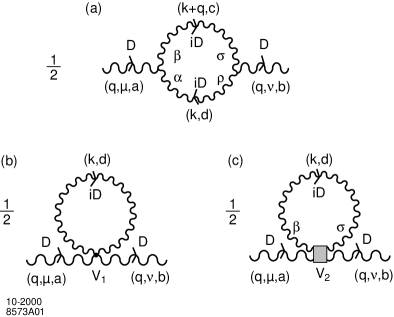
Figure 1: Yang-Mills self-energy to one loop. (a) Gluon self-energy diagram $\Pi^{\mu\nu}_{ab}(q)$; (b) tadpole diagram containing vertex $V_{1}$, vanishing in dimensional regularization; (c) non-vanishing tadpole diagram containing vertex $V_{2}$.

The propagator modification is given by

$$\delta_{ab}\frac{iD_{\lambda\delta}(q)}{q^{2}}+\delta_{aa^{\prime}}\frac{iD_{\lambda\mu}(q)}{q^{2}}\,\Pi^{\mu\nu}_{a^{\prime}b^{\prime}}(q)\,\delta_{b^{\prime}b}\frac{iD_{\nu\delta}(q)}{q^{2}}+\cdots$$ (28)

The contribution to the gluon polarization tensor $\Pi^{\mu\nu}_{ab}(q)$ coming solely from the three-gluon interaction is (Fig. 1a)

$$\Pi^{\mu\nu}_{ab}(q)\! = \!\int\!\frac{d^{d}k}{(2\pi)^{d}}\,\frac{1}{2}\,(-g_{d})^{2}\,f_{adc}\,f_{bcd}\,F^{\mu\alpha\beta}(-q,-k,k+q)$$ (29)

$$\qquad\qquad\qquad F^{\nu\sigma\rho}(q,-k-q,k)\,\frac{iD_{\beta\sigma}(k+q)}{(k+q)^{2}}\,\frac{iD_{\alpha\rho}(k)}{k^{2}}$$

$$= \frac{1}{2}\,g^{2}\,\delta_{ab}\,C_{A}\;\Pi^{\mu\nu}(q).$$

Here associated to the three outgoing momenta, $p_{1}^{\lambda}$, $p_{2}^{\mu}$, $p_{3}^{\nu}$, satisfying $(p_{1}+p_{2}+p_{3})^{\mu}=0$, we define

$$F_{\lambda\mu\nu}(p_{1},p_{2},p_{3})=(p_{1}-p_{2})_{\nu}g_{\lambda\mu}+(p_{2}-p_{3})_{\lambda}g_{\mu\nu}+(p_{3}-p_{1})_{\mu}g_{\nu\lambda}=-F_{\lambda\nu\mu}(p_{1},p_{3},p_{2}),$$ (30)

use $\,f_{adc}f_{bcd}=-C_{A}\delta_{ab}$ and write

$$\Pi^{\mu\nu}(q)=\mu^{4-d}\int\frac{d^{d}k}{(2\pi)^{d}}\frac{1}{[k^{2}+i\epsilon]\,[(k+q)^{2}+i\epsilon]}\;I^{\mu\nu}(q,k),$$ (31)

with

$$I^{\mu\nu}(q,k) = [-(2k+q)^{\mu}g^{\alpha\beta}+(k-q)^{\beta}g^{\mu\alpha}+(2q+k)^{\alpha}g^{\mu\beta}]D_{\alpha\rho}(k)$$ (32)

$$[-(2k+q)^{\nu}g^{\rho\sigma}+(k-q)^{\sigma}g^{\nu\rho}+(2q+k)^{\rho}g^{\nu\sigma}]D_{\sigma\beta}(k+q).$$

The dimensionless coupling is indicated by $g$ while $g_{d}=(\mu)^{\frac{4-d}{2}}g$ and $\mu$ indicates the mass parameter associated with the dimensional regularization which we will be adopting.

We first note that every internal gluon line carries a factor $D_{\mu\nu}$, and the polarization vector of an external gluon is $E^{\mu}_{(\perp)}=-D^{\mu}_{\perp}$. The object of interest relevant in the renormalization of the theory under consideration is clearly the combination $D_{\lambda\mu}(q)\,\Pi^{\mu\nu}_{ab}(q)\,D_{\nu\delta}(q)$. We may therefore use the transversity properties of $D^{\mu\nu}(q)$ to simplify the original expression and consider instead the following reduced expression for $I^{\mu\nu}$ in the integrand

$$I^{\mu\nu}(q,k) = [-(2k+q)^{\mu}g^{\alpha\beta}-2q^{\beta}g^{\mu\alpha}+2q^{\alpha}g^{\mu\beta}]D_{\alpha\rho}(k)$$ (33)

$$[-(2k+q)^{\nu}g^{\rho\sigma}-2q^{\sigma}g^{\nu\rho}+2q^{\rho}g^{\nu\sigma}]D_{\sigma\beta}(k+q).$$

Explicitly

$$I^{++} = 2(2k+q)^{+}(2k+q)^{+}$$

$$I^{+\perp} = I^{\perp+}=2(2k+q)^{+}(2k+q)^{\perp}+2(2k+q)^{+}\left[\frac{1}{(k+q)^{+}}-\frac{1}{k^{+}}\right]S_{\perp}$$

$$I^{\perp\perp^{\prime}} = 2\,(2k+q)^{\perp}(2k+q)^{\perp^{\prime}}$$ (34)

$$-2\,[(2k+q)_{\perp}S_{\perp^{\prime}}+(2k+q)_{\perp^{\prime}}S_{\perp}]\;\left[\frac{1}{(k+q)^{+}}-\frac{1}{k^{+}}\right]$$

$$-4\,g^{\perp\perp^{\prime}}\,S_{\perp}S_{\perp}\left[\frac{1}{{(k+q)^{+}}^{2}}+\frac{1}{{k^{+}}^{2}}\right]$$

$$-8\,S_{\perp}S_{\perp^{\prime}}\,\frac{1}{k^{+}\,(k+q)^{+}}$$

where

$$S_{\mu}\equiv S_{\mu}(k,q) = (k_{\mu}q^{+}-q_{\mu}k^{+})$$ (35)

$$= -S_{\mu}(q,k)=S_{\mu}(k+aq,q)=S_{\mu}(k,q+bk)$$

Here the properties $D^{\perp}_{\rho}(k)=[-\delta^{\perp}_{\rho}+(k^{\perp}/k^{+})\delta^{+}_{\rho}]$, $\,D^{\mu\nu}(k)D_{\mu\nu}(k)=2$, $\,D_{\lambda\mu}(q){D^{\mu}}_{\perp}(k)=-D_{\lambda\perp}(q)$ were used to simplify the expressions.

In order to carry out the renormalization procedure, we will need to isolate the divergent terms in the matrix element. We will adopt dimensional regularization since it preserves all gauge symmetries. The singularities in the Feynman propagators of the dynamical components $A_{\perp}$ and $\psi_{+}$ are given by the standard causal prescription. The $1/k^{+}$ singularity will be handled by the Mandelstam [36] and Leibbrandt [37] prescription in the l.c. gauge. A derivation of this prescription has also been given [21] in the context of equal-time canonical quantization. One can also justify the Mandelstam-Leibbrandt (ML) procedure by noting that in a two-dimensional massless theory on the LF, the causal prescription for the $k^{2}\approx 0$ singularity in $1/k^{2}\equiv 1/(2k^{+}k^{-})$ is identical to that given by the causal ML prescription for the $1/k^{+}$ singularity. Since we wish to have consistent analytic continuation in the number of dimensions $d$, the dimensional regularization plus ML prescription appears be a mathematically sound procedure.

The ML prescription is often written as

$$\frac{1}{q\cdot n}=\lim_{\epsilon\to 0}\frac{(q\cdot n^{*})}{(q\cdot n)(q\cdot n^{*})+i\epsilon}\,$$ (36)

where $\epsilon\to 0+\,$ and the light-like four-vector $n^{*}_{\mu}$ represents the dual of $n_{\mu}$ with the components given by, $n^{*}_{\mu}=\delta^{-}_{\mu}$. We recall that such a pair of null vectors, $n_{\mu}$ and $n^{*}_{\mu}$, arise quite naturally in the LF framework, for example, in the LF quantized QCD in covariant gauge [28], when we define the linearly independent set of four gauge field polarization vectors.

Unlike the principal value prescription for $1/k^{+}$, which would enter in conflict with the causal prescription for $1/k^{2}$, the causal $n^{*}_{\mu}$- prescription is consistent with both Wick rotation and power counting [22, 21].

The divergent part of $\Pi^{\mu\nu}$ may be computed straightforwardly employing the available list of integrals [22, 21]. We find

$$div\;\Pi^{++} = \frac{2}{3}\,{q^{+}}^{2}\,I^{div}$$

$$div\;\Pi^{+\perp} = -\frac{10}{3}\,q^{+}q^{\perp}\,I^{div}$$

$$div\;\Pi^{\perp\perp^{\prime}} = 2\,\left[\frac{11}{3}(q^{2}g^{\perp\perp^{\prime}}-q^{\perp}q^{\perp^{\prime}})-8\,q^{+}q^{-}g^{\perp\perp^{\prime}}\right]\,I^{div}$$ (37)

Here $\,(2\pi)^{4}I^{div}=2i\pi^{2}/{(4-d)}\to i\pi^{2}(2/\epsilon)$, with $d=(4-\epsilon)$, $\epsilon\to 0+$, is the pole term in the divergent integral

$$(2\pi)^{4}\;\mu^{4-d}\int\frac{d^{d}k}{(2\pi)^{d}}\;\frac{1}{k^{2}(k-q)^{2}}=i\pi^{2}\;\left[N_{\epsilon}-\ln\frac{-q^{2}}{\mu^{2}}+\cdots\right]+o(\epsilon)$$ (38)

where

$$N_{\epsilon}=\left[\frac{2}{\epsilon}-\gamma_{E}+\ln(4\pi)\right]$$

The expressions of $\,\Pi^{++}$, $\Pi^{+\perp}$ agree with the corresponding expressions computed in Ref. [22], in the conventional l.c. gauge QCD, where a different gluon propagator is used. However, the expression for $\Pi^{\perp\perp^{\prime}}$ is found to be different. As a consequence in the LF quantized theory we find covariant as well as noncovariant divergent terms in

$$D_{\lambda\mu}(q)\,\Pi^{\mu\nu}_{ab}(q)\,D_{\nu\delta}(q)=\frac{g^{2}}{16\pi^{2}}C_{A}\delta_{ab}\,(-\frac{11}{3}q^{2}+8q^{+}q^{-})\,\;i\,\left[N_{\epsilon}-\ln\frac{-q^{2}}{\mu^{2}}+\cdots\right]\;D_{\lambda\delta}(q)$$ (39)

Also, in view of the properties of $D_{\mu\nu}$, the computation of (39) does not require the evaluation of components other than those given in (37). We note also that

$$q_{\nu}I^{\mu\nu}=2\,(q^{2}+2k.q)\,\,\left[(2k+q)^{\mu}+(q^{\beta}g^{\mu\alpha}-q^{\alpha}g^{\mu\beta})\right]\,\,{D^{\rho}}_{\beta}(k+q)D_{\rho\alpha}(k).$$ (40)

The corresponding divergent part is shown to be

$$div\;q_{\nu}\ \Pi^{\nu\mu}(q)=-8\,q^{-}{q^{+}}^{2}\,{D^{\mu}}_{+}(q)\;I^{div},$$ (41)

which allows us to compute $div\,\,\Pi^{-+}(q)=\,(\frac{10}{3}q^{2}-\frac{22}{3}q^{+}q^{-})\,\,I^{div}$ by setting $\mu=+$.

The result (39) obtained here is different from the earlier l.c. gauge computations [22] in the conventional framework. The noncovariant piece $\,8q^{+}q^{-}\,N_{\epsilon}$, in (39), however, is compensated by an equal contribution but with opposite sign which arises from the tadpole graphs. The connection between tree-graph computations in the conventional light-cone gauge formalism and light-cone time-ordered perturbation theory have been discussed in refs. [40, 41, 42, 43]

The computation of the loop corrections to the gluon self-energy illustrates the essential difference between the light-front and conventional formalisms. There are two tadpole graphs (Figs. 1b and 1c) to be considered. The one associated with the four-gluon coupling $V_{1}$ gives a vanishing result, but the contribution coming from the instantaneous interaction $V_{2}(p_{1},p_{2},p_{3},p_{4})$ is found to be nonvanishing in dimensional regularization due to the momentum dependence of the vertex itself. The divergent part of the matrix element is easily reduced to

$$\mu^{4-d}\int\frac{d^{d}k}{(2\pi)^{d}}\,\frac{1}{2}(ig^{2})C_{A}\delta_{ab}\left[-(\frac{k^{+}-q^{+}}{k^{+}+q^{+}})^{2}-(\frac{k^{+}+q^{+}}{k^{+}-q^{+}})^{2}\right]\frac{iD^{\mu\nu}(k)}{k^{2}}D_{\lambda\mu}(q)D_{\nu\delta}(q)$$ (42)

$$= \frac{g^{2}}{16\pi^{2}}\,C_{A}\,\delta_{ab}\,(-8q^{+}q^{-})\,\;i\,\left[N_{\epsilon}-\ln\frac{-2q^{+}q^{-}}{\mu^{2}}+\cdots\right]\;\,D_{\lambda\delta}(q)$$

Here we made use of the useful identity $D_{\lambda\mu}(q)\,D^{\mu\nu}(k)\,D_{\nu\delta}(q)=D_{\nu\delta}(q)$ to arrive at the second line. The usual shift operation in dimensional regularization is used to bring the integral to another type of basic divergent integral [22] which is, however, noncovariant. On adding the tadpole contribution (42) to (39) the net coefficient of $(N_{\epsilon}+\ln\mu^{2})$ in the gluon self-energy correction is covariant, since the noncovariant $q^{+}q^{-}$ terms mutually cancel (see also Appendix C). Retaining only the pole term we find

$$D_{\lambda\mu}(q)\,\Pi^{\mu\nu}_{ab}(q)\,D_{\nu\delta}(q)=\frac{g^{2}}{16\pi^{2}}C_{A}\delta_{ab}\,(-\frac{11}{3}q^{2})\,\;i\,(\frac{2}{\epsilon})\,\,D_{\lambda\delta}(q).$$ (43)

The divergent part in (43) is $\propto q^{2}$ which ensures that the vanishing gluon mass remains unaltered due to the one-loop gluon self-energy correction.

The multiplicative renormalization constant $Z_{3}$ which corrects the gluon propagator is defined by

$$Z_{3}\,\;\delta_{ab}\frac{iD_{\lambda\delta}(q)}{q^{2}}=\delta_{ab}\frac{iD_{\lambda\delta}(q)}{q^{2}}+\delta_{aa^{\prime}}\frac{iD_{\lambda\mu}(q)}{q^{2}}\,\Pi^{\mu\nu}_{a^{\prime}b^{\prime}}(q)\,\delta_{b^{\prime}b}\frac{iD_{\nu\delta}(q)}{q^{2}}+\cdots$$ (44)

and we obtain

$$Z_{3}=1+\frac{g^{2}}{16\pi^{2}}\,C_{A}\,\frac{11}{3}\,\,(\frac{2}{\epsilon})$$ (45)

Vertex corrections:

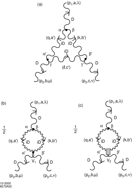
Figure 2: Three-gluon vertex diagrams. (a) Triangle diagram; (b) swordfish diagram containing vertex $V_{1}$; the other two diagrams are obtained by cyclic permutations of the external line indices; (c) swordfish diagrams containing vertex $V_{2}$; the other two diagrams are obtained by cyclic permutations of the external line indices.

In pure Yang-Mills theory the gluon vertex corrections to one-loop arise from the three-gluon interaction alone, the triangle diagram, (Fig. 2a) and from the two types of swordfish graphs (Figs. 2b and 2c) in which one of the two vertices carries a four-gluon interaction, which may be of type $V_{1}$ or type $V_{2}$, while the other one contains a three-gluon interaction. The complete vertex to order $g^{3}$ is written as

$$-gf_{abc}{\cal F}_{\lambda\mu\nu}=-gf_{abc}\,[F_{\lambda\mu\nu}+\Delta_{\lambda\mu\nu}](p_{1},p_{2},p_{3})=-gf_{abc}\,F_{\lambda\mu\nu}(p_{1},p_{2},p_{3})\,(1+\bar{\Delta})\ .$$ (46)

Consider first the triangle diagram. Since, as remarked before, each gluon line carries with it a factor of $D$ we will simplify the expressions right from the start making use also of the presence of the factor $\,D_{\lambda^{\prime}\lambda}(p_{1})D_{\mu^{\prime}\mu}(p_{2})D_{\nu^{\prime}\nu}(p_{3})$, coming from the external gluon lines. The matrix element for the one loop correction to order $g^{2}$ is written as

$$(-g_{d}^{2})\,(-\frac{1}{2}C_{A}\,f^{abc})\,(i)^{3}\;T^{\lambda\mu\nu}(p_{1},p_{2},p_{3})$$ (47)

where we have use $f_{aa^{\prime}b^{\prime}}f_{bb^{\prime}c^{\prime}}f_{cc^{\prime}a^{\prime}}=(C_{A}/2)f_{abc}$. A factor of $i$ comes from each of the gluon propagators and the expression for $T^{\lambda\mu\nu}(p_{1},p_{2},p_{3})$ is given by (Fig. 2a)

$$\int\frac{d^{d}q}{(2\pi)^{d}} \frac{D_{\alpha\alpha^{\prime}}(q)D_{\beta\beta^{\prime}}(k)D_{\gamma\gamma^{\prime}}(l)}{(q^{2}+i\epsilon)(k^{2}+i\epsilon)(l^{2}+i\epsilon)}[(p_{1}-q)^{\beta}g^{\alpha\lambda}+(q-k)^{\lambda}g^{\alpha\beta}+(k-p_{1})^{\alpha}g^{\lambda\beta}]$$ (48)

$$\qquad\qquad[(-q-p_{2})^{\gamma}g^{\alpha^{\prime}\mu}+(p_{2}-l)^{\alpha^{\prime}}g^{\gamma\mu}+(l+q)^{\mu}g^{\alpha^{\prime}\gamma}]$$

$$\qquad\qquad[(-k+l)^{\nu}g^{\beta^{\prime}\gamma^{\prime}}+(-l-p_{3})^{\beta^{\prime}}g^{\nu\gamma^{\prime}}+(p_{3}+k)^{\gamma^{\prime}}g^{\beta^{\prime}\nu}]$$

where $k=-(q+p_{1})$, $l=(q-p_{2})$, $p_{1}+p_{2}+p_{3}=0$ and the $D^{\prime}s$ associated with the external gluon lines are understood.

Proceeding as before we may consider instead the following reduced expression

$$8\int\frac{d^{d}q}{(2\pi)^{d}} \frac{D_{\alpha\alpha^{\prime}}(q)D_{\beta\beta^{\prime}}(k)D_{\gamma\gamma^{\prime}}(l)}{(q^{2}+i\epsilon)(k^{2}+i\epsilon)(l^{2}+i\epsilon)}[p_{1}^{\beta}g^{\alpha\lambda}+q^{\lambda}g^{\alpha\beta}-p_{1}^{\alpha}g^{\lambda\beta}]$$ (49)

$$[-p_{2}^{\gamma}g^{\alpha^{\prime}\mu}+p_{2}^{\alpha^{\prime}}g^{\gamma\mu}+q^{\mu}g^{\alpha^{\prime}\gamma}][-k^{\nu}g^{\beta^{\prime}\gamma^{\prime}}-p_{3}^{\beta^{\prime}}g^{\nu\gamma^{\prime}}+p_{3}^{\gamma^{\prime}}g^{\beta^{\prime}\nu}]$$

The divergent terms in $T^{\lambda\mu\nu}$ are then easily identified and may be rewritten as follows

$$8\int\frac{d^{d}q}{(2\pi)^{d}}\frac{1}{q^{2}k^{2}l^{2}} \left[2q^{\lambda}q^{\mu}k^{\nu}+p_{3}^{\alpha}q^{\lambda}q^{\mu}\{D^{\nu}_{\alpha}(l)-D^{\nu}_{\alpha}(k)\}\right.$$ (50)

$$\left.-k^{\nu}q^{\lambda}p_{2}^{\alpha}\{D^{\mu}_{\alpha}(q)-D^{\mu}_{\alpha}(l)\}-k^{\nu}q^{\mu}p_{1}^{\alpha}\{D^{\lambda}_{\alpha}(k)-D^{\lambda}_{\alpha}(q)\}\right].$$

The contribution to the divergent part comes solely from the first term, since the divergent terms coming from the noncovariant terms vanish. The divergent part of the one-loop correction from the triangle diagram has the form $\,-gf_{abc}\,F_{\lambda\mu\nu}(p_{1},p_{2},p_{3})\,{\bar{\Delta}}_{1}$ with

$$\bar{\Delta}_{1}=\frac{g^{2}}{16\pi^{2}}C_{A}\;(\frac{1}{3})\;\left[N_{\epsilon}-\ln\frac{Q^{2}}{\mu^{2}}+\cdots\right]$$ (51)

where $\,Q^{2}=-(p_{2}+p_{3})^{2}$. It is covariant and different from the one found [21, 22] in equal-time l.c. gauge framework where a different propagator is used, and the corresponding expressions contain noncovariant pieces.

The total contribution from each type of swordfish diagram comes from three similar diagrams, the two others being constructed from the first one by cyclic permutations of the set of labels of the three external gluon lines. The net divergent contribution following from the two types of diagrams is given by $\,-gf_{abc}\,F_{\lambda\mu\nu}(p_{1},p_{2},p_{3})\,{\bar{\Delta}}_{2}$ with

$$\bar{\Delta}_{2}=\frac{g^{2}}{16\pi^{2}}C_{A}\;(-4)\;\left[N_{\epsilon}-\ln\frac{Q^{2}}{\mu^{2}}+\cdots\right]$$ (52)

The noncovariant terms cancel out leading to the covariant result ${\bar{\Delta}}_{2}$ (see below). The gluon vertex renormalization constant $Z_{1}$ is defined by, $\bar{\Delta}=(\bar{\Delta}_{1}+\bar{\Delta}_{2})$,

$$-gf_{abc}{F}_{\lambda\mu\nu}(p_{1},p_{2},p_{3})\;\,\frac{1}{Z_{1}}=-gf_{abc}{F}_{\lambda\mu\nu}(p_{1},p_{2},p_{3})\;\,(1\,+\,\bar{\Delta})$$ (53)

and we obtain

$$\frac{1}{Z_{1}}=1-\frac{g^{2}}{16\pi^{2}}\,C_{A}\,(\frac{11}{3})\,(\frac{2}{\epsilon})$$ (54)

We find $Z_{1}=Z_{3}$ in our doubly transverse gauge framework in the l.c. gauge LF quantized theory. The gauge coupling constant renormalization constant $Z_{g}$, is defined by $\,Z_{g}={Z_{1}}/{(Z_{3})^{3/2}}$. In the lowest order perturbation theory it has the form

$$Z_{g}=\frac{Z_{1}}{(Z_{3})^{3/2}}=(Z_{3})^{-\frac{1}{2}}\approx\,1-\frac{g^{2}}{16\pi^{2}}\,C_{A}\,(\frac{11}{6})\;\,\,(\frac{2}{\epsilon})=1-{g^{2}}\,\beta_{0}\,(\frac{1}{\epsilon})$$ (55)

where $\,\beta_{0}=(1/{16\pi^{2}})\;({11\,C_{A}}/{3})\,>0$. It agrees with the result found [34, 35] in QCD, in the conventional instant form framework when the quark fields are ignored [44]. The computation of $\beta$-function and the discussion of the asymptotic freedom is made following the standard procedure [45, 52].

A sketch of the computation involved in the swordfish diagrams is presented here. The matrix element simplifies considerably due to the nice properties of the $D^{\prime}s$ leading to the reduced form

$$\frac{1}{2}\,(-ig_{d}^{2})\,\frac{1}{2}C_{A}\,f_{abc}\,\int\frac{d^{d}q}{(2\pi)^{d}}\frac{1}{q^{2}k^{2}}iD_{\alpha\alpha^{\prime}}(q)\,iD_{\beta,\beta^{\prime}}(k)$$

$$2\left[p_{1}^{\beta}g^{\alpha\lambda}-p_{1}^{\alpha}g^{\beta\lambda}+q^{\lambda}g^{\alpha\beta}\right]\,\left[Ag^{\alpha^{\prime}\mu}g^{\beta^{\prime}\nu}+Bg^{\alpha^{\prime}\nu}g^{\beta^{\prime}\mu}+Cg^{\alpha^{\prime}\beta^{\prime}}g^{\mu\nu}\right]$$ (56)

where

$$A=3-\frac{(q+p_{2})^{+}(p_{3}+k)^{+}}{(q-p_{2})^{+\,2}},\quad B=-3+\frac{(k+p_{2})^{+}(p_{3}+q)^{+}}{(q-p_{3})^{+\,2}},\quad C=2\frac{(k-q)^{+}(p_{3}-p_{2})^{+}}{(q+k)^{+\,2}}$$ (57)

with a multiplication by the factor $D_{\lambda^{\prime}\lambda}(p_{1})D_{\mu^{\prime}\mu}(p_{2})D_{\nu^{\prime}\nu}(p_{3})$ being understood. The integrand may be simplified further and recast as

$$p^{\rho}\left[\,-g^{\widetilde{\lambda}\widetilde{\mu}}\,(\,AD_{\rho}^{\widetilde{\nu}}(k)-BD_{\rho}^{\widetilde{\nu}}(q)\,)\,+g^{\widetilde{\lambda}\widetilde{\nu}}\,(\,AD_{\rho}^{\widetilde{\mu}}(q)-BD_{\rho}^{\widetilde{\mu}}(k)\,)\right.$$

$$\left.+Cg^{\mu\nu}\,(\,AD_{\rho}^{\widetilde{\lambda}}(q)-D_{\rho}^{\widetilde{\lambda}}(k)\,)\right]+\,q^{\lambda}g^{\widetilde{\mu}\widetilde{\nu}}\,(A+B)\,+\,2C\,q^{\lambda}\,g^{\mu\nu}$$ (58)

where $\widetilde{\mu}\equiv{\perp}=1,2$ only. The divergent terms then can be picked up straightforwardly. Some of them drop out if we use also $p_{1}^{\lambda}D_{\lambda^{\prime}\lambda}(p_{1})=0$ and $D_{-\mu}=0$. When we add to this result the two expressions obtained from the present one by the cyclic permutations of 3-tuples $(p_{1},\lambda,a)$, $(p_{2},\mu,b)$, and $(p_{3},\nu,c)$, the noncovariant pieces drop out, leading to the covariant expression for $\bar{\Delta}_{2}$ given above.

The divergent terms arising from each type of the swordfish graphs contain covariant as well as noncovariant pieces. The contribution corresponding to the usual four-gluon vertex $V_{1}$ in our framework agrees with the one found in the earlier l.c. gauge computations [21, 22], in the conventional framework. It thus gives us a consistency check of our calculations, since the computation here is insensitive to the $n_{\mu}n_{\nu}k^{2}/{k^{+}}^{2}$ term in our gauge propagator. The doubly transverse gauge propagator of the LF quantized theory greatly simplifies the computation: in compensation for the few extra interaction vertices, there are no ghost interactions.

5.3 Gluon Self-Energy corrections from Quark loop

For each flavor $f$ of quark the net gluon self-energy contribution arising from a quark loop is found to acquire the usual form

$$\Pi^{(F)\mu\nu}_{aa^{\prime}}=(-1)\,(ig)^{2}\,\sum_{ij}t^{a}_{ij}t^{a^{\prime}}_{ji}\,\,\mu^{4-d}\,(i)^{2}\,\int\frac{d^{d}k}{(2\pi)^{d}}\;\frac{Tr({\not k}+m_{f})\gamma^{\mu}({\not k}+{\not q}+m_{f})\gamma^{\nu}}{[k^{2}-{m_{f}}^{2}]\,[(k+q)^{2}-{m_{f}}^{2}]}.$$ (59)

where the factor $D_{\lambda\mu}(q)D_{\nu\delta}(q)$ is understood. It is easily shown that the noncovariant contributions either vanish or are mutually cancelled. Hence

$$div\;D_{\lambda\mu}(q)\,\Pi^{(F)\mu\nu}_{aa^{\prime}}\,D_{\nu\delta}(q) = \frac{g^{2}}{16\pi^{2}}\,\,\delta_{aa^{\prime}}\,\,T_{F}\,\,(\,\frac{4}{3}\,q^{2})\;D_{\lambda\delta}(q)$$ (60)

$$i\,\left[N_{\epsilon}-6\int_{0}^{1}dx\,x(1-x)\,\ln\,\frac{m_{f}^{2}-x(1-x)\,q^{2}}{\mu^{2}}\right]$$

where $\sum_{ij}t^{a}_{ij}t^{a^{\prime}}_{ji}=T_{F}\delta_{aa^{\prime}}$. The contributions from $\Pi^{(F)-\nu}_{aa^{\prime}}$ or $\Pi^{(F)\mu-}_{aa^{\prime}}$ are automatically suppressed in view of $D_{\mu-}=0$, as they should, since $A_{-}=0$ in the l.c. gauge. We have used also

$$D_{\lambda\mu}(q)\,\,(q^{2}g^{\mu\nu}-q^{\mu}q^{\nu})\,\,D_{\nu\delta}(q)=-q^{2}D_{\lambda\delta}(q).$$ (61)

For the total number $n_{f}$ of massless quarks we find

$$div\;D_{\lambda\mu}(q)\,\Pi^{(F)\mu\nu}_{aa^{\prime}}\,D_{\nu\delta}(q)=\frac{g^{2}}{16\pi^{2}}\,\delta_{aa^{\prime}}\,T_{F}\,(\frac{4}{3}\,n_{f}\,q^{2})\,i\,\left[N_{\epsilon}-\ln\frac{-q^{2}}{\mu^{2}}+\cdots\right]\;D_{\lambda\delta}(q).$$ (62)

The net contribution to coefficient of the pole term in the gluon self-energy becomes

$$div\;D_{\lambda\mu}(q)\,\left[\Pi^{\mu\nu}_{aa^{\prime}}+\Pi^{(F)\mu\nu}_{aa^{\prime}}\right]\,D_{\nu\delta}(q) = \frac{g^{2}}{16\pi^{2}}\,\delta_{aa^{\prime}}\,\,q^{2}\,\,\left(-\frac{11}{3}C_{A}+\frac{4}{3}\,n_{f}\,T_{f}\right)$$ (63)

$$\quad i\,(\frac{2}{\epsilon})\,D_{\lambda\delta}(q).$$

which leads to

$$Z_{3}=1+\frac{g^{2}}{16\pi^{2}}\,\left(\frac{11}{3}C_{A}-\frac{4}{3}\,n_{f}\,T_{F}\right)\,(\frac{2}{\epsilon})$$ (64)

with

$${Z_{3}}^{-\frac{1}{2}}=1-\frac{g^{2}}{16\pi^{2}}\,\left(\frac{11}{6}C_{A}-\frac{2}{3}\,n_{f}\,T_{F}\right)\,(\frac{2}{\epsilon})$$ (65)

in our ghost free l.c. gauge LF quantized QCD framework. We also did not perform any renormalization of the gauge parameter, required in the conventional covariant gauge theory framework. A complete discussion of QCD in our framework will be given elsewhere [46].

6 Conclusions

The canonical quantization of l.c. gauge QCD in the front form theory has been derived employing the Dirac procedure to construct a self-consistent LF Hamiltonian theory. The formulation begins with the gauge-fixed BRS invariant quantum action, but the final result is ghost-free. The interaction Hamiltonian is obtained in a simple form by retaining the dependent components $A_{+}$ and $\psi_{-}$. Its form closely resembles the interaction Hamiltonian of covariant theory, except for the presence of instantaneous interactions which are analogous to the Coulomb interactions in transverse gauge. The Dyson-Wick perturbation theory expansion based on equal-LF-time ordering is then constructed in a manner which allows one to perform high order computations in straightforward fashion. Our formulation of the light-front Hamiltonian matches the rules of light-front-time-ordered perturbation theory [16].

In our formulation of gauge theory, the free gauge field satisfies the Lorentz condition as an operator equation as well as the light-cone gauge constraint. Since the propagator of the massless gauge field is doubly transverse both with respect to the four-momentum and the four-vector $n_{\mu}$ of gauge direction, the propagating gluons have only two physical degrees of freedom, and no ghost fields need to be considered. The physical transverse polarization vectors of the gluons may be conveniently identified as $E^{\mu}_{(\perp)}(k)\equiv-D^{\mu}_{\perp}(k)$ so that each gluon line, external or internal, carries with it a factor of $D_{\mu\nu}$. The remarkable properties of these factors give rise to much simplification already at the start of computations.

Unitarity relations [47] such as the optical theorem are manifest within each Feynman diagram, rather than as a consequence of cancelations over sets of diagrams [48]. This allows one to construct effective charges analogous to the Gell Mann-Low running coupling of QED based on the structure of self-energy diagrams using the pinch technique[49]. Since the absorptive part of these contributions are based on physical cross sections, one can define a physical and analytic renormalization scheme for QCD.

The instantaneous interactions, in fact, are interesting by themselves. For example, the semi-classical limit of Thomson scattering is revealed at the tree level in the l.c. or covariant gauge [28] on the LF. This is relevant since a systematic procedure to obtain the semi-classical limit seems to be lacking in the front form theory. The LF framework may be useful also for obtaining the non-relativistic limit of a relativistic field theory, for example, in the context of chiral perturbation theory. This is an alternative to the conventional framework where a functional integral technique and the Foldy-Wouthuysen transformation is employed.

It is worth stressing that the doubly transverse propagator obtained here follows from the straightforward application of the well-tested standard Dirac method for constructing Hamiltonian formulation for constrained dynamical systems. It differs from the singly transverse propagator usually used in the literature in the context of equal-time l.c. gauge QCD. In the equal-time formalism the last term $n^{\mu}n^{\nu}k^{2}\over n\cdot kn\cdot k$ of the doubly-transverse gauge propagator is absent so that both transverse and longitudinal gluonic modes propagate. The instantaneous interaction terms generated by l.c. gauge in the LF are also not present in the analysis of instant form noncovariant gauge QCD based on functional integral quantization. Even when one allows for counterterms obtained by imposing [21, 22, 30] constraints of covariance or by requiring an extended BRS symmetry, the gauge propagators employed in that framework do not possess the very useful properties carried by the doubly transverse LF framework. We have illustrated the correspondence between the two formulations of light-cone gauge with a simple tree-graph calculation of electron-muon scattering in QED. The instantaneous terms in the LF interaction Hamiltonian restore the manifest Lorentz covariance of the matrix element which was broken by the noncovariant gauge and the noncovariant terms in the doubly-transverse gauge propagator. The same is found true in nonabelian gauge theory.

The singularities in the noncovariant pieces of the field propagators may be defined using the causal l.c. gauge ML prescription for $1/k^{+}$. The power-counting rules in l.c. gauge then become similar [50, 21, 51] to those found in covariant gauge theory as the illustrations show. We have demonstrated explicitly the equality $Z_{1}=Z_{3}$ and $Z_{g}={(Z_{3})}^{-\frac{1}{2}}$ at one loop in Yang-Mills theory. This is expected to be true in higher orders as well. Also because of the Slavnov-Taylor identities [52], the corrections to the $qqg$ vertex would be compensated by the ones arising from the quark field renormalization; such that the coupling constant renormalization arises only from the gluonic self-energy.

Computations in our ghost-free framework require comparable effort as calculations in covariant gauge because of the remarkable simplifications arising due to the doubly transverse l.c. gauge propagator. Higher-loop computations should be possible in our formalism by making advantageous use of the techniques [50] which have recently been developed to handle multi-loop integrals involving noncovariant integrands.

The renormalization procedure of LF quantized gauge theory in l.c.g. is thus similar to that of conventional covariant gauge theory. The additional interaction terms are in a sense the appropriate counterterms which arise naturally in the canonical quantization in the LF framework. It is straightforward to show this in QED; a complete discussion for QCD will be given elsewhere [46].

It is worth remarking that we have made an ad hoc choice of only one (of the family) of the characteristic LF hyperplanes, $x^{+}=const.$, in order to quantize the theory. The conclusions reached here and in the earlier works [11, 28] confirm the conjecture [11] concerning the irrelevance in the quantized theory of the fact that the hyperplanes $x^{\pm}=0$ constitute characteristic surfaces of hyperbolic partial differential equation. The Hamiltonian version can clearly be implemented in DLCQ [29] which has been shown [53] to have a continuum limit. There is no loss of causality in DLCQ when the infinite volume limit is properly handled [54]. We also note that nonperturbative computations are often done on the LF in the closely related (l.c.) gauge $\partial_{-}A_{-}\approx 0$, such as to demonstrate [12] the existence of the condensate or $\theta$-vacua in the Schwinger model.

Appendix A

The Feynman Rules

The Dyson-Wick perturbation theory expansion on the LF can be realized in momentum space by employing the Fourier transform of the fields and the propagators. Many of the rules of the Feynman diagrams, for example, the symmetry factor $1/2$ for gluon loop, a minus sign associated with fermionic loops etc., are the same as those found in the conventional covariant framework [52]. There are some differences:   for example, the external quark line now carries a factor $\theta(p^{+})\sqrt{{m}/{p^{+}}}$ while the external gluon line a factor $\theta(q^{+})/\sqrt{2q^{+}}\;$ or that the Lorentz invariant phase space factor is now $\int d^{2}p^{\perp}dp^{+}\,\theta(p^{+})/(2p^{+})$. The external gluon line carries the polarization vector $E^{\mu(\perp)}(q)=E^{\mu}_{(\perp)}=-D^{\mu}_{\perp}(q)$. Its properties and the sum over the two polarization states are given Section 3. The notation for the quark field is given in Appendix B. Some of the momentum space vertices, used in Section 5, are collected below and others can be derived easily.

Gluon propagator:

$$i\delta^{ab}\frac{D_{\mu\nu}(q)}{q^{2}+i\epsilon},\quad{\rm with}\quad\,D_{\mu\nu}(q)=\left(-g_{\mu\nu}+\frac{n_{\mu}q_{\nu}+q_{\mu}n_{\nu}}{n\cdot q}-\frac{q^{2}}{(n\cdot q)^{2}}n_{\mu}n_{\nu}\right),$$

where $q_{\mu}$ is the gluon 4-momentum and $n_{\mu}$ is the gauge direction. We choose $n_{\mu}\equiv\delta^{+}_{\mu}$ and $n^{*}_{\mu}\equiv\delta^{-}_{\mu}$, the dual of $n_{\mu}$. The useful properties of the projector $D_{\mu\nu}$ are given in Eqs. (16-19).

Quark propagator:

$$i\delta_{ij}S(p),\quad{\rm with}\quad S(p)\equiv\frac{\not{p}+m}{p^{2}-m^{2}+i\epsilon}-\frac{\gamma^{+}}{2p^{+}}=\frac{N(p)}{p^{2}-m^{2}+i\epsilon}\,\qquad\epsilon>0,$$

where $p_{\mu}$ is the quark 4-momentum, $i$ and $j$ are color indices and $N(p)=({\not{p}}+m)$ $-(p^{2}-m^{2}){\gamma^{+}}/{2p^{+}}$. The noncovariant second term on the right hand side is present only in the propagator of the nondynamical dependent field $\psi_{-}$. Its contribution, for example, to gluon self-energy (63) is, however, compensated by that arising from the fourth term in (24).

Quark-quark-gluon vertex factor:

$$ig\,\gamma^{\mu}t^{a}$$

3-gluon vertex factor:

$$-g\,f_{abc}\,F_{\lambda\mu\nu}(p_{1},p_{2},p_{3})$$

Here $(p_{1},{\lambda},a)$, $(p_{2},{\mu},b)$, and $(p_{3},{\nu},c)$, label the three gluons at the vertex with outgoing momenta $p_{1}^{\lambda}$, $p_{2}^{\mu}$ and $p_{3}^{\nu}$ with the associated gauge indices $a$, $b$ and $c$ respectively. Also $F_{\lambda\mu\nu}(p_{1},p_{2},p_{3})=(p_{1}-p_{2})_{\nu}g_{\lambda\mu}+(p_{2}-p_{3})_{\lambda}g_{\mu\nu}+(p_{3}-p_{1})_{\mu}g_{\nu\lambda}=-F_{\lambda\nu\mu}(p_{1},p_{3},p_{2})$ and $p_{1}+p_{2}+p_{3}=0$.

4-gluon vertex factors:

There are two types of 4-gluon vertices in this framework. The ${V_{1}\,}^{abcd}_{\alpha\mu\nu\beta}$ is the usual momentum-independent four-gluon vertex of the covariant gauge theory, while ${V_{2}\,}^{abcd}_{\alpha\mu\nu\beta}(p_{1},p_{2},p_{3},p_{4})$ is a new vertex generated by l.c. gauge LF quantized QCD, with the momentum dependence as well, coming from the last term in the interaction Hamiltonian (36):

$${V_{1}\,}^{abcd}_{\alpha\mu\nu\beta} = -ig^{2}\left[f^{eab}f^{ecd}(g^{\alpha\nu}g^{\beta\mu}-g^{\alpha\beta}g^{\mu\nu})\right.$$

$$\left.+f^{eac}f^{ebd}(g^{\alpha\mu}g^{\beta\nu}-g^{\alpha\beta}g^{\mu\nu})\right.$$

$$\left.+f^{ead}f^{ecb}(g^{\alpha\nu}g^{\beta\mu}-g^{\alpha\mu}g^{\beta\nu})\right]$$

and

$${V_{2}\,}^{abcd}_{\alpha\mu\nu\beta}(p_{1},p_{2},p_{3},p_{4}) = +ig^{2}\left[f^{eab}f^{ecd}g^{\alpha\mu}g^{\beta\nu}\,\frac{(p_{1}-p_{2})^{+}(p_{3}-p_{4})^{+}}{(p_{1}+p_{2})^{+2}}\right.$$

$$\left.+f^{eac}f^{ebd}g^{\alpha\nu}g^{\beta\mu}\,\frac{(p_{1}-p_{3})^{+}(p_{2}-p_{4})^{+}}{(p_{1}+p_{3})^{+2}}\right.$$

$$\left.+f^{ead}f^{ecb}g^{\alpha\beta}g^{\mu\nu}\,\frac{(p_{1}-p_{4})^{+}(p_{3}-p_{2})^{+}}{(p_{1}+p_{4})^{+2}}\right]$$

Here $(p_{1},\alpha,a)$, $(p_{2},\mu,b)$, $(p_{3},\nu,c)$, and $(p_{4},\beta,d)$ indicate the four outgoing gluons at the vertex with $p_{1}+p_{2}+p_{3}+p_{4}=0$.

Appendix B

Spinor Field on the LF

The notation for gamma matrices is as given in Bjorken and Drell and $\,\gamma^{\pm}=(\gamma^{0}\pm\gamma^{3})/{\sqrt{2}}\,$ which satisfy $\,({\gamma^{+}})^{2}=({\gamma^{-}})^{2}=0$. The $\,\Lambda^{\pm}={1\over 2}\gamma^{\mp}\gamma^{\pm}={1\over\sqrt{2}}\gamma^{0}\gamma^{\pm}\,$ are hermitian projection operators. The spinor field on the LF is decomposed naturally into $\,{\pm}\,$ projections: $\,\psi_{\pm}=\Lambda^{\pm}\psi\,$, $\,{\bar{\psi}}_{\pm}={\bar{\psi}}\Lambda^{\mp}\,$, $\psi=\psi_{+}+\psi_{-}$, and ${\bar{\psi}}=\psi^{{\dagger}}\gamma^{0}$ $={\bar{\psi}}_{+}+{\bar{\psi}}_{-}$, $\,\gamma^{\pm}\psi_{\mp}=0$, $\,{\bar{\psi}}_{\pm}\gamma^{\mp}=0$, etc.

The Fourier transform of the free spinor field [28] is

$$\psi(x)={1\over{\sqrt{(2\pi)^{3}}}}\sum_{r={\pm}}\int d^{2}p^{\perp}dp^{+}\,\theta(p^{+}){\sqrt{m\over p^{+}}}\left[b^{(r)}(p){u^{(r)}}(p)e^{-ip\cdot x}+d^{{{\dagger}}{(r)}}(p){v^{(r)}}(p)e^{ip\cdot x}\right]$$

where

$$u^{(r)}(p)=\frac{1}{({{\sqrt{2}}p^{+}m})^{1\over 2}}\left[{\sqrt{2}}p^{+}\Lambda^{+}+(m+\gamma^{\perp}p_{\perp})\Lambda^{-}\right]\widetilde{u}^{(r)}$$

and the constant spinors $\widetilde{u}^{(r)}$ satisfy $\gamma^{0}\widetilde{u}^{(r)}=\widetilde{u}^{(r)}$ and $\Sigma_{3}\widetilde{u}^{(r)}=r\widetilde{u}^{(r)}$ with $\Sigma_{3}=i\gamma^{1}\gamma^{2}$ and $r=\pm$. The normalization and the completeness relations are:

$$\bar{u}^{(r)}(p)u^{(s)}(p)=\delta_{rs}=-\bar{v}^{(r)}(p)v^{(s)}(p)$$

$$\sum_{r=\pm}u^{(r)}(p){\bar{u}}^{(r)}(p)=\frac{(\not p+m)}{{2m}}$$

$$\sum_{r=\pm}v^{(r)}(p){\bar{v}}^{(r)}(p)=\frac{(\not p-m)}{{2m}}$$

and C is the charge conjugation matrix [24] while $v^{(r)}(p)\equiv{u^{(r)}(p)_{c}}=C{\gamma^{0}}^{T}u^{(r)}(p)^{*}$.

The $\Lambda^{+}$ projection of is by construction very simple, ${u^{(r)}}_{+}(p)={({\sqrt{2}}p^{+}/m)}^{1\over 2}(\Lambda^{+}{\widetilde{u}^{(r)}})$. The ${u^{(r)}}_{+}(p)$ are eigenstates of $\Sigma_{3}$ as well, while the $\widetilde{u}^{(r)}$ correspond to rest frame spinors when ${\sqrt{2}}p^{\pm}=m$.

The free propagator for the independent component $\psi_{+}$ is

$$\left\langle{0|T({\psi^{i}}_{+}(x){\psi^{{\dagger}j}}_{+}(0))|0}\right\rangle={{i\delta^{ij}}\over{(2\pi)^{4}}}\int d^{4}q\;{{{\sqrt{2}}q^{+}\,\Lambda^{+}}\over{(q^{2}-m^{2}+i\epsilon)}}\,e^{-iq.x}$$

and we recall that $2i\partial_{-}\psi_{-}=(i\gamma^{\perp}\partial_{\perp}+m)\gamma^{+}\psi_{+}$.

A detailed discussion of the properties of Dirac, Majorana and Weyl spinor fields, helicity and spin operators, and the generalized chiral invariance of massive Dirac equation on the LF may be found in Ref. [5].

Appendix C

The self-consistent canonical quantization of the gauge theory requires one to fix the gauge and add ghost fields in order to ensure BRS symmetry. One must also choose a regularization procedure in order to compute and manipulate the divergent integrals present in the momentum space representation of the theory. In our context dimensional regularization is convenient since it preserves the gauge (and BRS) symmetry, thus making the task of renormalization simpler. However the regularization procedure may break essential properties of a physical theory, such as unitarity and introduce ghost degrees of freedom at an intermediate stage. One hopes that at the end of computations when the regularization is removed that we recover the features associated with the physical theory represented by the original Lagrangian. It is worth recalling the case of Chiral Schwinger model where the regularization ambiguity itself leaves behind an arbitrary parameter in the theory, which is physical and unitary only for a certain range of the values of that parameter. It was also shown a long time ago [55] that the Pauli-Villars method of regularization corresponds to the introduction of (regularization-dependent) ghost degrees of freedom in the original theory. The dimensional regularization procedure along with the ML prescription may also give rise to the additional (hidden regularization-dependent) ghost contributions to the divergent integrals [38]. The noncovariant $\ln(-2q^{+}q^{-})$ contribution in Eq. (42) to the gluon self-energy has an unconventional branch cut when compared to the normal threshold branch point in Eq. (39). It is an indication, in the dimensional regularization scheme with ML prescription, of ghost states that do not propagate in the transverse direction. The sign of the cut in Eq. (42) is that of asymptotic freedom, i.e., ghostly. In the gluon self-energy the sign of the coefficient of $\ln(-q^{2})$ term in Eq. (39) is consistent with the spectral representation of Källen-Lehmann but that of $\ln(-2q^{+}q^{-})$ term is opposite. In the renormalization of the vertex functions, only the $\ln(-q^{2})$ terms are found.

We note that the renormalization factors of Yang-Mills theory in Feynman gauge employing dimensional regularization are

$$Z_{3}=1+\frac{g^{2}}{16\pi^{2}}C_{A}\,\frac{10}{3}\,\frac{1}{\epsilon}\;>1,\qquad\qquad Z_{1}=1+\frac{g^{2}}{16\pi^{2}}C_{A}\,\frac{4}{3}\,\frac{1}{\epsilon}\;>1,$$

while

$${\tilde{Z}}_{3}=1+\frac{g^{2}}{16\pi^{2}}C_{A}\,\frac{1}{\epsilon}\;>1,\qquad\qquad{\tilde{Z}}_{1}=1-\frac{g^{2}}{16\pi^{2}}C_{A}\,\frac{1}{\epsilon}\;<1,$$

such that $Z_{1}/Z_{3}={\tilde{Z}}_{1}/{\tilde{Z}}_{3}.$ The result is the same coupling constant renormalization as in our LF framework

$$Z_{g}=\frac{Z_{1}}{{Z_{3}}^{3/2}}=\frac{{\tilde{Z}}_{1}}{{\tilde{Z}}_{3}\sqrt{Z_{3}}}=1-\frac{g^{2}}{16\pi^{2}}C_{A}\,(\frac{11}{6})\,N_{\epsilon}\;<1.$$

Here ${\tilde{Z}}$ refer to the Faddeev-Popov ghost fields of the covariant gauge theory. We find that in this framework $Z_{3}>1$, just as in the LF framework presented where, in addition, $Z_{g}={Z_{3}}^{-1/2}$. This corresponds to the asymptotic freedom property of dimensionally regularized nonabelian gauge theories due to the three gluon’s nonlinear self-interaction.

If only physical degrees of freedom are present, wavefunction renormalization requires $Z_{3}<1$; i.e, the probability that the gluon is a bare gluon must be less than one. As pointed out by Thorn [8], the fact that $Z_{3}>1$ in Yang-Mills theory is in conflict with the unitarity and the positivity of the Källen-Lehmann spectral representation of the gluon propagator. Note that in our light-front formulation of the doubly transverse light-cone gauge, the renormalization of the three-gluon vertex receives a crucial one-loop contribution from the instantaneous $V_{2}$ interaction as illustrated by the swordfish diagram of figure 2(c). [This diagram is missing from the renormalization of the proper three-gluon vertex in the conventional light-cone gauge formalism since it is classified as one-particle reducible.] Similarly, the tadpole graph 1(c) from $V_{2}$ must be included in computation of the gluon self energy. Such a term does not have a conventional two-particle cut or Källen-Lehmann dispersion representation, thus allowing for $Z^{g}_{3}>1$ [39]. We note also that our gauge propagator is not diagonal like that in the Feynman gauge.

References

• [1] P.A.M. Dirac, Rev. Mod. Phys. 21, 392 (1949).
• [2] S. J. Brodsky, Light-Cone Quantized QCD and Novel Hadron Phenomenology, SLAC-PUB-7645, 1997; S. J. Brodsky and H. C. Pauli, Light-Cone Quantization and QCD, Lecture Notes in Physics, vol. 396, eds., H. Mitter et al., Springer-Verlag, Berlin, 1991.
• [3] S. J. Brodsky, H. Pauli and S. S. Pinsky, Phys. Rept. 301, 299 (1998).
• [4] K. G. Wilson et al., Phys. Rev. D49, 6720 (1994); K. G. Wilson, Nucl. Phys. B (proc. Suppl.) 17, 82 (1990); R. J. Perry, A. Harindranath, and K. G. Wilson, Phys. Rev. Lett. 65, 2959 (1990).
• [5] P. P. Srivastava, Perspectives of Light-Front Quantum Field Theory: Some New Results, in Quantum Field Theory: A 20th Century Profile, pgs. 437-478, Ed. A.N. Mitra, Indian National Science Academy and Hidustan Book Agency, New Delhi, 2000; SLAC preprint, SLAC-PUB-8219, August 1999; hep-ph/9908492, 11450. See also Nuovo Cimento A107, 549 (1994) and [2, 3, 4, 5] for earlier references.
• [6] D. Bigatti and L. Susskind, Review of matrix theory, hep-th/9712072; Phys. Lett. B425, 351 (1998), hep-th/9711063.
• [7] E. Witten, Commun. Math. Phys.92, 455 (1984).
• [8] C. B. Thorn, Phys. Rev. D20, 1934 (1979).
• [9] On physical grounds we must require the cluster decomposition principle, which requires that distant experiments give uncorrelated results. See, S. Weinberg, in Conceptual foundations of quantum field theory, Ed. T. Y. Cao, Cambridge University Press, 1999.
• [10] P. P. Srivastava, Chiral boson theory on the light-front, SLAC preprint, SLAC-PUB-8252; hep-ph/9909412.
• [11] P. P. Srivastava, Phys. Letts. B448, 68 (1999); hep-th/9811225.
• [12] P. P. Srivastava, Mod. Phys. Letts. A13, 1223 (1998); hep-th/9610149.
• [13] J. B. Kogut and D. E. Soper, Phys. Rev. D1, 2901 (1970); D. E. Soper, Phys. Rev. D4, 1620 (1971).
• [14] T. M. Yan, Phys. Rev. D7, 1760 (1973) and the earlier references contained therein.
• [15] J. D. Bjorken, J. B. Kogut and D. E. Soper, Phys. Rev. D3, 1382 (1971).
• [16] G. P. Lepage and S. J. Brodsky, Phys. Rev. D22, 2157 (1980).
• [17] K. Bering, J. S. Rozowsky and C. B. Thorn, Phys. Rev. D 61, 045007 (2000) [hep-th/9909141].
• [18] J. S. Rozowsky and C. B. Thorn, Phys. Rev. D 60, 045001 (1999) [hep-th/9902145].
• [19] J. S. Rozowsky and C. B. Thorn, Phys. Rev. Lett. 85, 1614 (2000) [hep-th/0003301].
• [20] S. Pinsky and U. Trittmann, Phys. Rev. D 62, 087701 (2000) [hep-th/0005055].
• [21] A. Bassetto, G. Nardelli and R. Soldati, Yang-Mills Theories in Algebraic Non-Covariant Gauges, World Scientific, 1991; A. Bassetto, M. Dalbosco, and R. Soldati, Phys. Rev. D36, 3138 (1987). See also Ref. [30] and A. Bassetto, G. Heinrich, Z. Kunszt, and W. Vogelsang, Phys. Rev. D58, 94020 (1998); hep-ph/9805283
• [22] G. Leibbrandt, Noncovariant Gauges, Quantization of Yang-Mills and Chern-Simons theory in axial type gauges, World Scientific, Singapore, 1994; Rev. Mod. Phys. 59, 1067 (1987); Nucl. Phys. B310, 405 (1988). See also Ref. [50]
• [23] R. J. Perry, Light-front quantum chromodynamics, nucl-th/9901080.
• [24] See, C. Itzykson and J. B. Zuber, Quantum Field Theory, McGraw-Hill, 1980; J. D. Bjorken and S. D. Drell, Relativistic Quantum Fields, McGraw-Hill, 1965; L. H. Ryder, Quantum Field Theory, Cambridge University Press, 1996.
• [25] A report on these results were presented at the parallel session on Recent Developments in Field Theory, Talk 15b-03, at XXXth Intl. Conference on High Energy Physics-ICHEP2000, July27- August 2, 2000, Osaka, Japan. Condensed version to be published in the Proceedings, World Scientific, Singapore.
• [26] P.A.M. Dirac, Lectures in Quantum Mechanics, Belfer Graduate School of Science, Yeshiva University Press, New York, 1964; Can. J. Math. 2, 129 (1950); E.C.G. Sudarshan and N. Mukunda, Classical Dynamics: a modern perspective, Wiley, NY, 1974. See also L. Faddeev and R. Jackiw, Phys. Rev. Lett. 60, 1692 (1988).
• [27] For an introduction to the Dirac method, see S. Weinberg, in The Quantum Theory of Fields, Cambridge University Press, 1995.
• [28] P. P. Srivastava and S. J. Brodsky, Phys. Rev. D61, 25013 (2000); SLAC preprint SLAC-PUB-8168, hep-ph/9906423.
• [29] H. C. Pauli and S. J. Brodsky, Phys. Rev. D32, 2001 (1985).
• [30] Physical and Nonstandard Gauges, Eds., P. Gaigg, W. Kummer and M. Schweda, Lecture Notes in Physics, vol. 361, Springer-Verlag, 1990.
• [31] P. P. Srivastava, Nuovo Cimento A 108, 35 (1995); hep-th/9412204-205.
• [32] C. Becchi, A. Rouet and R. Stora, Ann. Phys. (N.Y.) 98, 287 (1976).
• [33] R. Floreanini and R. Jackiw, Phys. Rev. Lett. 59, 1873 (1987).
• [34] D.J. Gross and F. Wilczek, Phys. Rev. Lett. 30, 1343 (1973).
• [35] H.D. Politzer, Phys. Rev. Lett. 30, 1346 (1973).
• [36] S. Mandelstam, Nucl. Phys. B213, 149 (1983).
• [37] G. Leibbrandt, Phys. Rev. D29, 1699 (1984).
• [38] M. Morara, R. Soldati and G. McCartor, hep-th/9909200.
• [39] We thank Dae Sung Hwang for conversations on this point.
• [40] S. A. Paston, V. A. Franke and E. V. Prokhvatilov, Theor. Math. Phys. 120, 1164 (1999) [hep-th/0002062].
• [41] A. Harindranath and W. Zhang, Phys. Rev. D 48, 4903 (1993).
• [42] W. Zhang and A. Harindranath, Phys. Rev. D 48, 4881 (1993).
• [43] N. E. Ligterink and B. L. Bakker, Phys. Rev. D 52, 5954 (1995) [hep-ph/9412315].
• [44] We note that on the LF we again have $Z_{3},Z_{1}>1$ as in the conventional Feynman gauge QCD theory. See Appendix C.
• [45] See, [27]; J. Collins, Renormalization, Cambridge University Press, Cambridge, 1984.
• [46] in preparation.
• [47] For example, the discontinuity (imaginary part) in the gluon self-energy is computed as follows. We write in Eq.(29)
$$\int\frac{d^{4}k}{(2\pi)^{4}}=\int\frac{d^{4}p_{1}}{(2\pi)^{4}}\int\frac{d^{4}p_{2}}{(2\pi)^{4}}\,(2\pi)^{4}\,\delta^{4}(p_{1}+p_{2}-q),$$
where $p_{1}=-k,\;p_{2}=(k+q)$. In each of the two propagators replace [28]:  $\,1/(p_{i}^{2}+i\epsilon)\to-2\pi\,i\delta(p_{i}^{2})\,\theta(p_{i}^{+})\theta(p_{i}^{-})$ and express, using (18), $D_{\mu\nu}(p_{i})=\sum_{(\perp_{i})}{E^{(\perp_{i})}}_{\mu}(p_{i}){E^{(\perp_{i})}}_{\nu}(p_{i})$, $\,i=1,2$, as sum over the two transverse polarizations of physical gluons. We find that the discontinuity is proportional to $\theta(q^{2})$. For time-like $q^{2}$ the imaginary parts of $\ln(-q^{2})$ and $\ln(-2q^{+}q^{-})$ which appear in Eqs. (39) and (42) respectively are the same. It results in the mutual cancellation in the contribution to the imaginary part of the gluon self-energy, which are multiplied by the noncovariant factor $q^{+}q^{-}$. Similar procedure may be followed to check the unitarity relation for the self-energy corrections arising from quark-loop.
• [48] J. Papavassiliou, E. de Rafael and N. J. Watson, Nucl. Phys.  B503, 79 (1997), hep-ph/9612237.
• [49] J. M. Cornwall, Phys. Rev. D 26, 1453 (1982); N. J. Watson, Phys. Lett. B349, 155 (1995); J. Papavassiliou, Phys. Rev. D 62, 045006 (2000); S. J. Brodsky, E. Gardi, G. Grunberg, and J. Rathsman, hep-ph/0002065.
• [50] G. Leibbrandt and J. D. Williams, Nucl. Phys. B566, 373 (2000), hep-th/9911207 and the references cited therein.
• [51] S. J. Brodsky, R. Roskies and R. Suaya, Phys. Rev. D8, 4574 (1973).
• [52] See, M. E. Peskin and D. V. Schroeder, An Introduction to Quantum Field Theory, Addison-Wesley, 1995; L.D. Fadeyev, and A.A. Slavnov, Gauge Fields, Benjamin, NY, 1980; P. Langacker, Physics Reports, 72, 185 (1981).
• [53] P.P. Srivastava, Light-front quantization and Spontaneous Symmetry Breaking- Discretized formulation , Ohio State Univ. preprint 92-0173, SLAC PPF 9222, April 1992; AIP Conf. Proceedings No. 272, XXVI Intl. Conf. on High Energy Physics, Dallas, TX, August 6-12, pg. 2125 (1992), Ed., J.R. Sanford; hep-th/9412193. See also Hadron Physics 94, p. 253, Eds. V. Herscovitz et al., World Scientific, Singapore, 1995; hep-th/9412204, 205.
• [54] D. Chakrabarti et al., Numerical Experiment in DLCQ: Microcausality, Continuum limit and All That, hep-th/9910108.
• [55] S.N. Gupta, Proc. Phys. Soc. A63, 681 (1950); A66, 129 (1953); P. Srivastava, Phys. Lett. 149B, 135 (1984).