Renormalization Group Flow Equations for the scalar $O(N)$ theory

Abstract

Self-consistent new renormalization group flow equations for an $O(N)$-symmetric scalar theory are approximated in next-to-leading order of the derivative expansion. The Wilson-Fisher fixed point in three dimensions is analyzed in detail and various critical exponents are calculated.

1 Introduction and conclusion

In this talk we present novel nonperturbative flow equations for an $O(N)$-symmetric scalar theory in next-to-leading order of the derivative expansion. Based on the Wilsonian Renormalization Group method also known as the Exact Renormalization Group (ERG) approach we combine a Schwinger proper time regularization scheme with a perturbative treatment in order to obtain self-consistent RG flow equations. We investigate in detail the nontrivial Wilson-Fisher fixed point in three dimensions and determine universal quantities such as the critical exponents $\eta$, $\nu$, $\beta$ and $\delta$ independently for arbitrary numbers of field components $N$ without resorting to any polynomial truncations. For this approach the typical and inherent analytical threshold functions in the flow equations, which describe the continuous decoupling of the massive modes from the RG evolution enable a direct and smooth linkage between the four-dimensional system at zero temperature and the critical $O(N)$ universal behavior near the critical temperature $T_{c}$. The dimensional reduction phenomenon is embedded in the threshold functions in a very transparent way.[1, 2] The prediction of the universal critical exponents is one of the great achievements of the ERG methods but they may also be applied to other systems e.g. with a first-order phase transition.[3] All ERG equations are equivalent up to the choice of the regulator or cutoff function. For instance Polchinski’s equations in the limit of a sharp momentum cutoff are the Wegner-Houghton equations and are equivalent to Wilson’s equations.[4] In order to extract physical relevant quantities from the ERG equations which are complicated highly non-linear functional equations one has to employ an appropriate approximation or truncation scheme. The ERG equations themselves are by construction scheme independent but this need not be true any longer in specific truncations. Thus, different realizations of the cutoff function or regulator for the ERG equations yield an uncertainty in the determination of universal quantities. To leading order the critical exponents are scheme inpedendent but in next-to-leading order the results become scheme dependent. This makes it particularly difficult to determine uniquely the critical exponent $\eta$. For instance in four dimensions the sharp cutoff Wegner-Houghton equation predicts the proper field anomalous dimension $\eta$ in next-to-leading order in the derivative expansion but it fails at the Wilson-Fisher fixed point in three dimensions.[5] We propose a smooth cutoff version of the ERG based on a heat-kernel regularization which should overcome these difficulties and obtain remarkable precise values for the anomalous dimension $\eta$ in a very simple uniform wavefunction renormalization approximation by neglecting the field dependence in $Z_{k}$. In order to provide an estimate of the scheme dependence we determine several critical exponents for different implementations of the smooth cutoff functions and find a rapid convergence to stable values that are in good agreement with entirely different approaches. Another criterion for estimating the scheme dependence may be based on the minimum sensitivity principle which we do not further pursue in this work.[6] The next section is devoted to a brief review of the derivation of the flow equations for the potential $U_{k}$ and the coefficient $Z_{k}$ of the lowest-order derivative term.[7]

2 The flow equations with a proper time regularization

As an illustrative example and as a test we apply the method with a proper time regulator to an $O(N)$ scalar theory. In the ultraviolet (UV) region of the theory at the scale $\Lambda$ of the order of $1$ GeV we consider the following effective Lagrangian L_Λ= 12 ( ∂_μ→Φ )^2 + λ4 ( →Φ^2 - Φ_0^2 )^2 with the $N$-component vector $\vec{\Phi}=(\Phi_{1},\Phi_{2},\ldots,\Phi_{N})$. The field $\Phi_{0}^{2}$ denotes the minimum of the potential. The expansion in powers of momenta of the effective action up to order ${\cal O}(\partial^{4})$ reads Γ[→Φ] =∫d^d x { -U(→Φ^2 ) +12 Z_1 ( →Φ^2 ) ( ∂_μ →Φ )^2 + 12 Z_2 ( →Φ^2 ) (→Φ ∂_μ →Φ )^2 }  . The perturbative one-loop contribution to the effective action yields formally a non-local logarithm which we regularize by a proper-time regularization resulting in a finite local action. We implement a multiplicative, a priori unknown, blocking or smearing function $f_{k}(\tau)$ which governs the coarse-graining in the proper-time integrand. In this way the sharp proper-time cutoff is replaced by a smooth one and the scale $k$ acts as an infrared cutoff separating the low- and high-momentum modes of the fields. After introducing a complete set of plane wave states in the heat kernel this procedure yields the following $d$-dimensional effective action[8] Γ[→Φ] = -12 ∫d^d x ∫_0^∞ d ττ f_k ∫ddp(2π)d tr  e^- τ( p^2 - 2ip_μ ∂_μ - ∂^2 +V_ij” (Φ)) with the shorthand notation $V_{ij}^{\prime\prime}(\Phi)=\frac{\delta^{2}V}{\delta\Phi_{i}\delta\Phi_{j}}$ for the $(N\times N)$-matrix valued second derivative of the $O(N)$-symmetric potential $V$ at the UV scale $\Lambda$. The second derivative is given by $V_{ij}^{\prime\prime}=\lambda\left(\vec{\Phi}^{2}-\Phi_{0}^{2}\right)\delta_{ij}+2\lambda\Phi_{i}\Phi_{j}$. The trace in Eq. (2) runs over the $N$ fields and can be evaluated analytically with standard techniques. In order to find the next-to-leading order of the effective action we expand $\exp\left[-\tau\left(-2ip_{\mu}\partial_{\mu}-\partial^{2}+V^{\prime\prime}\right)\right]$ in powers of derivatives up to second order. To this order the action separates into two parts Γ_2 = Γ^(0) + Γ^(2)with $\Gamma^{(0)}$ denoting the one-loop potential contribution (containing no derivatives) and $\Gamma^{(2)}$ the second-order contribution (containing two derivatives). Comparing the expansion coefficients $U$, $Z_{1}$, $Z_{2}$ of the effective action (2) with the corresponding terms in $\Gamma_{2}$ we can extract the effective potential contribution and the wavefunction renormalization contributions. In order to simplify the work drastically we perform a uniform wavefunction renormalization by neglecting the field dependence and consider only one wavefunction renormalization $Z_{1}=Z_{k}$. It turns out that this simple approximation already describes all qualitative features at the phase transition. The desired self-consistent flow equations are obtained by differentiation of the equations with respect to the infrared scale $k$ followed by the substitution $V\to U_{k}$ on the right-hand side. This replacement has an analogy to the Schwinger-Dyson self-consistent resummation. The structure of the flow equations depends on the choice of the blocking functions but the universal physical results which are obtained by solving these flow equations towards the infrared should not depend on the specific choice. The regulator essentially governs the way how the irrelevant operators of the theory are integrated over. Here we chose for any integer $M\geq 0$ the following form for the derivative of the blocking functions k ∂fk(M)(τ)∂k ∼-2 (τZ_k k^2)^(M+2) e^-τZ_k k^2 . and obtain e.g. for the blocking function with $M=1$ the rescaled dimensionless flow equations in $d$ dimensions

$$k\frac{\partial u_{k}({\phi}^{2})}{\partial k} = -du_{k}+(d-2+\eta){\phi}^{2}u^{\prime}_{k}+\frac{S_{d}}{d}\left[\frac{1}{1+2u^{\prime}_{k}+4{\phi}^{2}u^{\prime\prime}_{k}}+\frac{N-1}{1+2u^{\prime}_{k}}\right]$$ (1)

$$-\frac{k}{Z_{k}}\frac{\partial Z_{k}}{\partial k} = \left.\frac{2S_{d}}{{\phi}^{2}d}\left[1+\frac{1}{(1+4{\phi}^{2}u^{\prime\prime}_{k})^{2}}+\frac{1}{2{\phi}^{2}u^{\prime\prime}_{k}}\left(\frac{1}{1+4{\phi}^{2}u^{\prime\prime}_{k}}-1\right)\right]\right|_{\phi=\phi_{0}}\ ,$$ (2)

$$\mbox{where}\qquad S_{d}=2/\Gamma(d/2)(4\pi)^{d/2},\ {\phi}^{2} := k^{-(d-2+\eta)}\Phi^{2}_{k}\quad\mbox{and}\quad u_{k}({\phi}^{2}):=k^{-d}U_{k}({\phi}^{2})\hfill\ \$$

and we have introduced the anomalous dimension $\eta=-k\partial_{k}\ln Z_{k}$. A prime on the potential denotes differentiation with respect to ${\phi}^{2}$. Because we have omitted the field dependence of the wavefunction renormalization the flow equation (2) for $Z_{k}$ has to be evaluated at the minimum of the potential $\phi_{0}$.

3 Results

In order to test the approximations described above we solve the coupled system of flow equations by discretization of the field $\phi^{2}$ for a general, not truncated potential $u_{k}(\phi^{2})$ numerically on a grid by a fifth-order Runge Kutta algorithm for each grid point. Details can be found in the work by O. Bohr et al.[2]. The flow equations (1) and (2) are in a scale-independent form and, due to the dimensional reduction phenomenon, we do not need to use the finite temperature version of the flow equations at the critical temperature. We can directly link the $O(N)$ universal behavior near $T_{c}$ with the physics at zero temperature and therefore it is sufficient to employ only the three-dimensional zero-temperature equations in order to investigate the critical regime of the phase transition. In this way we circumvent the evaluation of Matsubara sums for the investigation of the critical point. A second-order phase transition involves an infrared fixed point of the RG transformations. Thus, the physics close to the phase transition is scale invariant and the critical behavior should be described by a scale-independent solution. This is demonstrated in Fig. 1 where the $k$-evolution towards zero of the dimensionless minimum $\phi^{2}_{0}$ of the potential for different initial values near the critical value at the UV scale $k=\Lambda$ is shown. The dashed line indicates the $k$-independent constant (fixed point) scaling solution while the evolution near the critical value deviates either towards the spontaneously broken ($\phi^{2}_{0}\neq 0$) or the symmetric ($\phi^{2}_{0}=0$) phase. Of course, not only the minimum $\phi^{2}_{0}$ but all quantities show a scaling behaviour.

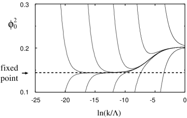
Figure 1: The evolution of the dimensionless minimum towards the scaling solution.

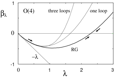
Figure 2: $\beta_{\lambda}(\lambda)$ for the $O(4)$-model compared to a one- and three-loop $\epsilon$-expansion. The arrows indicate the flow w.r.t. the scale $k$ towards the infrared.

For dimensions less than four two fixed points are present in the system and can be identified by zeros in the beta functions. In general it is difficult to calculate the zeros since this requires knowledge of the physics beyond perturbation theory. In Fig. 2 the curve, denoted by RG, shows the beta function $\beta_{\lambda}$ of the quartic coupling for an $O(4)$-model within our approach. This result is compared with a one- and three-loop $\epsilon$-expansion. Thus, the nontrivial infrared-stable Wilson-Fisher fixed point can clearly by identified around $\lambda^{*}\sim 2.3$ for $N=4$.

Table 1: Critical exponents for various $N$. Our results (RG) are compared with lattice simulations, $\epsilon$-expansion ($\epsilon$) and a perturbative calculation ($SPS$).

$\begin{array}[]{c}\\ \end{array}$	$\eta$	$\delta$	$\nu$	$\beta$
N=0 $\begin{array}[]{c}\mbox{RG}\\ \mbox{lattice}\\ \epsilon\\ SPS\end{array}$	$\begin{array}[]{c}0.039\\ 0.041(25)\\ 0.032(3)\\ 0.027(4)\end{array}$	$\begin{array}[]{c}4.77\\ 4.77(14)\\ 4.81(2)\\ 4.84(3)\end{array}$	$\begin{array}[]{c}0.59\\ 0.592(3)\\ 0.588(2)\\ 0.588(2)\end{array}$	$\begin{array}[]{c}0.30\\ 0.308(6)\\ 0.304(2)\\ 0.302(2)\end{array}$
N=1 $\begin{array}[]{c}\mbox{RG}\\ \mbox{lattice}\\ \epsilon\\ SPS\end{array}$	$\begin{array}[]{c}0.044\\ 0.044(31)\\ 0.038(3)\\ 0.032(3)\end{array}$	$\begin{array}[]{c}4.75\\ 4.75(17)\\ 4.78(2)\\ 4.81(2)\end{array}$	$\begin{array}[]{c}0.64\\ 0.631(2)\\ 0.631(2)\\ 0.630(2)\end{array}$	$\begin{array}[]{c}0.32\\ 0.329(9)\\ 0.327(2)\\ 0.325(2)\end{array}$
N=4 $\begin{array}[]{c}\mbox{RG}\\ \mbox{lattice}\\ \epsilon\end{array}$	$\begin{array}[]{c}0.037\\ 0.0254(38)\\ 0.03(1)\end{array}$	$\begin{array}[]{c}4.79\\ 4.851(22)\\ 4.82(6)\end{array}$	$\begin{array}[]{c}0.78\\ 0.7479(90)\\ 0.73(2)\end{array}$	$\begin{array}[]{c}0.40\\ 0.3836(46)\\ 0.38(1)\end{array}$
N=100 $\begin{array}[]{c}\mbox{RG}\end{array}$	$\begin{array}[]{c}0.0025\end{array}$	$\begin{array}[]{c}4.99\end{array}$	$\begin{array}[]{c}0.99\end{array}$	$\begin{array}[]{c}0.49\end{array}$
$\begin{array}[]{c}\\ \end{array}$large-$N$	0	5	1.0	0.5

Note, that this value depends on the particular form of the flow equations encoded in the choice of the blocking function. However, an expansion e.g. of the beta function $\beta_{\lambda}$ in powers of the coupling yields in three dimensions $\beta_{\lambda}=-\lambda+\frac{2(N+8)}{3\pi^{2}}\lambda^{2}+{\cal O}(\lambda^{3})$ which agrees with the first two terms of an $\epsilon$-expansion as it should. Corresponding to the large-$N$ limit the fixed point $\lambda^{*}$ tends to zero merging with the trivial Gaussian fixed point. Linearizing the flow about the Wilson-Fisher fixed point allows the determination of the critical exponents by means of finding the corresponding eigenvalues. We have calculated the exponents $\beta$, $\delta$, $\nu$ and $\eta$ independently, which allows to test the well-known scaling relations among the critical exponents. Their values are listed in Tab. 1 for various $N$. The agreement with different approaches is a further confirmation of our approximations described above. One realizes explicitly the convergence of all calculated critical exponents to the large-$N$ values quoted in the last line of Tab. 1. In the large-$N$ limit the local potential approximation becomes exact and the anomalous dimension $\eta$ vanishes.

In order to investigate the scheme dependence of the non-truncated set of flow equations for the full potential we derive flow equations for the blocking functions defined in Eq. (2) with $M=0,1,2$ and neglect the wavefunction renormalization. As an example we take $N=4$ and calculate again the critical exponent $\nu$ and $\beta$. The dependence of these critical exponents on the blocking function of order $M$ is shown in Tab. 2.

Table 2: The critical exponents $\nu$ and $\beta$ for $N=4$ with different blocking functions $f^{(M)}_{k}(\tau)$ (without wavefunction renormalization).

$M$	$\nu$	$\beta$
0	0.853	0.42
1	0.815	0.405
2	0.814	0.403

A small systematic decrease in the values with the order $M$ is observed. This behaviour is also seen in the results of Refs. [5, 9] where the dependence of the parameter $M$ practically vanishes for bigger values of $M$. Already for $M\geq 1$ we do not see any difference in the second significant digit. Going beyond the Local Potential Approximation (LPA) and taking the wavefunction renormalization into account this tendency becomes more stable with the order $M$. An analysis of the blocking functions $f_{k}^{(M)}$ with increasing $M$ shows that the regulator has the effect of selecting smaller and smaller momentum shells.[5] It represents for very large $M$-values a kind of sharp cutoff limit which, however, cannot be directly linked to the sharp cutoff Wegner-Houghton equation. This means that a deeper understanding of the relation between this novel approach concerning the heat kernel cutoff and other formulations of the ERG is still an important outstanding issue. So far we and other authors have to restrict the comparisons of the different methods to numerical results only.[5, 10]

References

- [1] J. Berges, N. Tetradis and Ch. Wetterich, hep-ph/0005122; J. Berges, D.-U. Jungnickel and Ch. Wetterich, Phys. Rev. D59 (1999) 034010.
- [2] O. Bohr, B.-J. Schaefer and J. Wambach, hep-ph/0007098.
- [3] see e.g. N. Tetradis, Phys. Lett. B431 (1998) 380 and these proceedings.
- [4] F.J. Wegner and A. Houghton, Phys. Rev. A8 (1973) 401; K. Wilson and J. Kogut, Phys. Rep. C12 (1974) 75; J. Polchinski, Nucl. Phys. B231 (1984) 269.
- [5] A. Bonanno and D. Zappal, hep-th/0010095 and these proceedings.
- [6] D. Litim, Phys. Lett. B486 (2000) 92 and these proceedings; R.D. Ball et al., Phys. Lett. B347 (1995) 80.
- [7] A. Bonanno, V. Branchina, H. Mohrbach and D. Zappal, Phys. Rev. D60 (1999) 065009.
- [8] B.-J. Schaefer and H.-J. Pirner, Nucl. Phys. A627 (1997) 481; Nucl. Phys. A660 (1999) 439.
- [9] G. Papp, B.-J. Schaefer, H.-J. Pirner and J. Wambach, Phys. Rev. D61 (2000) 096002.
- [10] S.-B. Liao, C.-Y. Lin and M. Strickland, hep-th/0010100.