Abstract

The overlap representation of skewed parton distributions (SPDs) is discussed and applications to wide-angle Compton scattering and electroproduction of mesons are presented. The amplitudes for these processes factorise into parton-level subprocess amplitudes and form factors representing $1/x$-moments of SPDs.

Key-words: skewed parton distributions, wide-angle exclusive reactions

Invited talk presented at the XV International Seminar on High Energy Physics Problems, Dubna (September 2000)

Abstract

The overlap representation of skewed parton distributions (SPDs) is discussed and applications to wide-angle Compton scattering and electroproduction of mesons are presented. The amplitudes for these processes factorise into parton-level subprocess amplitudes and form factors representing $1/x$-moments of SPDs.

Key-words: skewed parton distributions, wide-angle exclusive reactions

1 Introduction

Interactions of protons with high energy electromagnetic probes, either electrons (i.e., virtual photons) or real photons, are desribed by the handbag diagram shown in Fig. 1. Depending on the virtuality of the incoming photon, $Q^{2}$, and on the momentum transfer from the incoming to the outgoing proton, $t$, different processes are described by the handbag diagram: For forward scattering, $t=0$, with highly virtual photons, $Q^{2}\gg\Lambda^{2}$, (where $\Lambda$ is a typical hadronic scale of order 1 GeV) the cutted diagram represents the total cross section for the absorption of virtual photons by protons. This is the domain of deep inelastic lepton-proton scattering from which process we learned about the ordinary unpolarised, $q(x)$, and polarised, $\Delta q(x)$, parton distribution functions (PDFs). Considering for definiteness outgoing real photons, the handbag diagram describes deeply virtual Compton scattering for large $Q^{2}$ and small $-t$ and, for large $-t$ (and $-u$) but small $Q^{2}$, real and virtual wide-angle Compton scattering. Common to all these processes are soft proton matrix elements which represent generalised PDFs or, as termed frequently, SPDs. The same matrix elements also occur in the form factors of the proton and in deeply virtual as well as wide-angle electroproduction of mesons. In the following I am going to discuss properties of the SPDs and their representation in terms of light-cone wave function (LCWF) overlaps. The role of the SPDs in wide-angle exclusive scattering will also be explained.

2 Skewed parton distributions

Parameterizing the kinematics of the SPD as in Fig. 1, one can define the following fractions of light-cone plus momentum components

$$\xi=\frac{(p-p^{\prime})^{+}}{(p+p^{\prime})^{+}}\,,\qquad\bar{x}=\frac{(k+k^{\prime})^{+}}{(p+p^{\prime})^{+}}\,,\qquad x=\frac{\bar{x}+\xi}{1+\xi}\,,\qquad x^{\prime}=\frac{\bar{x}-\xi}{1-\xi}\,,$$ (1)

where $\xi$ is termed the skewedness parameter. $x(x^{\prime})$ is the momentum fraction the emitted (absorbed) parton carries. The SPDs $H^{q}(\bar{x},\xi;t)$ and $E^{q}(\bar{x},\xi;t)$ for a quark of flavour $q$ are defined as the Fourier transform of a bilocal product of field operators sandwiched between proton states [1]

$${\cal H}_{\lambda^{\prime}\lambda}^{q} \equiv \frac{1}{2\sqrt{1-\xi^{2}}}\;\sum_{c}\int\frac{{\rm d}z^{-}}{2\pi}\;e^{i\,\bar{x}\,\bar{p}^{\,+}z^{-}}\;\langle p^{\,\prime},\lambda^{\prime}|\,\overline{\psi}_{q}^{\,c}(-\bar{z}/2)\,\gamma^{+}\,\psi_{q}^{\,c}(\bar{z}/2)\,|p,\lambda\rangle$$ (2)

$$= \frac{\overline{u}(p^{\,\prime},\lambda^{\prime})\gamma^{+}u(p,\lambda)}{2\bar{p}^{\,+}\sqrt{1-\xi^{2}}}\;H^{q}(\bar{x},\xi;t)+\frac{\overline{u}(p^{\,\prime},\lambda^{\prime}){i\sigma^{+\alpha}\Delta_{\alpha}}u(p,\lambda)}{4m\,\bar{p}^{\,+}\sqrt{1-\xi^{2}}}\;E^{q}(\bar{x},\xi;t)\,,$$

(in $A^{+}=0$ gauge, $t=\Delta^{2}$). $\lambda$, $\lambda^{\prime}$ denote the proton helicities and $\bar{z}$ is a shorthand notation for $[0,z^{-},{\bf 0}_{\perp}]$. The decomposition (2) defines the two SPDs in analogy to the Dirac, $F_{1}$, and Pauli, $F_{2}$, form factors of the proton. The corresponding matrix element of $\gamma^{+}\gamma_{5}$ defines two further SPDs, $\widetilde{H}^{q}$ and $\widetilde{E}^{q}$. For $\xi<\bar{x}\leq 1$ the SPDs describe the emission of a quark with momentum fraction $x>0$ from the proton and the absorption of a quark with momentum fraction $x^{\prime}>0$. In the region $-\xi\leq\bar{x}\leq\xi$ the proton emits a quark-antiquark pair ($x\geq 0$, $x^{\prime}\leq 0$) and is left as a proton. Finally, for $-1\leq\bar{x}<-\xi$ the SPD describes the emission and absorption of antiquarks ($x,x^{\prime}<0$). Antiquark SPDs can be defined by $H^{\bar{q}}(\bar{x},\xi;t)=-H^{q}(-\bar{x},\xi;t)$ and so on. The extension to gluon SPDs is straightforward.

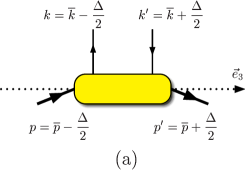
Figure 1: The handbag diagram (left) and the kinematics for SPDs (right).

Reduction formulas relate the SPDs to the ordinary PDFs:

$$H^{q}(\bar{x},0;0) = q(\bar{x}),\phantom{x}\qquad\widetilde{H}^{q}(\bar{x},0;0)\;=\;\Delta q(\bar{x})$$

$$H^{g}(\bar{x},0;0) = \bar{x}g(\bar{x}),\qquad\widetilde{H}^{g}(\bar{x},0;0)\;=\;\bar{x}\Delta g(\bar{x})\,.$$ (3)

The other SPDs, $E^{q}$ and $\widetilde{E}^{q}$, are not accessible to deep inelastic lepton-nucleon scattering. Integrating the SPDs over $\bar{x}$ one obtains the contribution of flavour $q$ quarks to the proton form factors, e.g.,

$$F_{1}^{q}(t)=\langle\bar{x}^{0}\rangle=\int_{-1}^{1}{\rm d}\bar{x}\,H^{q}(\bar{x},\xi;t)\,.$$ (4)

The $\langle\bar{x}^{0}\rangle$-moments of the other SPDs, $E^{q}$, $\widetilde{H}^{q}$ and $\widetilde{E}^{q}$, provide contributions to the Pauli, the axial, and the pseudoscalar form factors, respectively. Multiplying, for instance, $F^{q}_{1}$ by the appropriate electric charges and summing over all flavours, one obtains the full Dirac form factor.

As shown in [2, 3] (see also [4]), the SPDs possess a representation in terms of LCWF overlaps which is a generalization of the famous Drell-Yan formula for the electromagnetic form factors [5]. Its derivation starts from a Fock decomposition of the proton state

$$\left|p,\lambda\right\rangle=\sum_{N,\beta}\int[{{\rm d}}x]_{N}[{{\rm d}}^{2}{\bf k}_{\perp}]_{N}\;\Psi_{N,\beta}^{\lambda}(r)\;\left|N,\beta;k_{1},\ldots,k_{N}\right\rangle\,,$$ (5)

where $\beta$ labels the different $N$-particle Fock states and $[{{\rm d}}x]_{N}[{{\rm d}}^{2}{\bf k}_{\perp}]_{N}$ is the $N$-particle integration measure. In the framework of light-cone quantisation one can show that, in the region $\xi<\bar{x}\leq 1$, the SPDs are represented by the diagonal $N\to N$ overlaps

$${\cal H}_{\lambda^{\prime}\lambda}^{q(N\to N)}=\sqrt{1-\xi^{2}}^{\,1-N}\;\sum_{\beta=\beta^{\prime}}\;\sum_{j}\delta_{s_{j}q}\;\int[{\rm d}\bar{x}]_{N}[{\rm d}^{2}\bar{\bf k}_{\perp}]_{N}\;\delta\left(\bar{x}-\bar{x}_{j}\right)\;\Psi_{N,\beta^{\prime}}^{*\,\lambda^{\prime}}(\hat{r}^{\prime})\,\Psi_{N,\beta}^{\lambda}(\tilde{r})\,,$$ (6)

where the arguments of the LCWFs read ($j$ labels the active quark, $i\neq j$ the spectators)

$$\tilde{x}_{i}=\frac{\bar{x}_{i}}{1+\xi}\,,\quad\tilde{\bf k}_{\perp i}=\bar{\bf k}_{\perp i}+\frac{\bar{x}_{i}}{1+\xi}\,\frac{{\bf\Delta}_{\perp}}{2}\,,\quad\tilde{x}_{j}=\frac{\bar{x}_{j}+\xi}{1+\xi}\,,\quad\tilde{\bf k}_{\perp j}=\bar{\bf k}_{\perp j}-\frac{1-\bar{x}_{j}}{1+\xi}\,\frac{{\bf\Delta}_{\perp}}{2}\,,$$

$$\hat{x}^{\prime}_{i}=\frac{\bar{x}_{i}}{1-\xi}\,,\quad\hat{\bf k}^{\prime}_{\perp i}=\bar{\bf k}^{\phantom{.}}_{\perp i}-\frac{\bar{x}_{i}}{1-\xi}\,\frac{{\bf\Delta}_{\perp}}{2}\,,\quad\hat{x}^{\prime}_{j}=\frac{\bar{x}_{j}-\xi}{1-\xi}\,,\quad\hat{\bf k}^{\prime}_{\perp j}=\bar{\bf k}^{\phantom{.}}_{\perp j}+\frac{1-\bar{x}_{j}}{1-\xi}\,\frac{{\bf\Delta}_{\perp}}{2}\,.$$ (7)

The overlap representation of the matrix element $\widetilde{{\cal H}}^{q(N\to N)}_{\lambda^{\prime}\lambda}$ is, except of an additional factor $\rm{sign}(\mu_{j})$ (where $\mu_{j}$ is the helicity of the active parton), also given by (6). For the gluon SPDs there is an additional factor $\sqrt{\bar{x}^{2}-\xi^{2}}$. The overlap representation in the region $-1\leq\bar{x}<-\xi$ is given by (6) too with the replacement of $\delta(\bar{x}-\bar{x}_{j})$ by $\delta(\bar{x}+\bar{x}_{j})$. The region $-\xi\leq\bar{x}\leq\xi$ is described by non-diagonal $N+1\to N-1$ overlaps. I refrain from displaying that formula here and refer to Ref. [3, 4].

In the region $\xi<\bar{x}\leq 1$ the overlap representation satisfies the positivity constraints

$$\left|{\cal H}^{q}_{\lambda^{\prime}\lambda}\right|\leq\frac{1}{\sqrt{1-\xi^{2}}}\;\sqrt{q(x)\;q(x^{\prime})}\,,\qquad\left|{\cal H}^{g}_{\lambda^{\prime}\lambda}\right|\leq\sqrt{\frac{\bar{x}^{2}-\xi^{2}}{1-\xi^{2}}}\;\sqrt{g(x)\;g(x^{\prime})}\,,$$ (8)

first derived in [6]. I.e. we obtain bounds for the combination $H^{q(g)}-\xi^{2}/(1-\xi^{2})\,E^{q(g)}={\cal H}_{\lambda\lambda}$ and for $E^{q(g)}$ ($\propto{\cal H}_{\lambda-\lambda}$) [3]. In previous work [6, 2] the $E^{q(g)}$ term in the bound for proton helicity non-flip transitions have been overlooked. The combinations ${\cal H}^{q(g)}_{\lambda^{\prime}\lambda}\pm\widetilde{{\cal H}}^{q(g)}_{\lambda^{\prime}\lambda}$ are analogously bounded by the PDFs for definite helicities [3].

Considering the special case $\Delta_{\perp}=\xi=0$, $\lambda^{\prime}=\lambda$, Eq. (6) and the corresponding one for $\widetilde{{\cal H}}^{q}_{\lambda\lambda}$ reduce to the LCWF representation of the ordinary PDFs, $q$ and $\Delta q$, respectively. Thus, the reduction formulas (2) are automatically satisfied. Taking $\xi=0$ and integrating (6) over $\bar{x}$ the ordinary Drell-Yan formula [5] is recovered. In the same manner LCWF representations of the other proton from factors are obtained.

3 The soft physics approach

Let us now turn to wide-angle exclusive scattering, defined by $s,-t,-u\gg\Lambda$, $Q^{2}$ fixed. As is well-known, for asymptotically large momentum transfer these processes are controlled by the perturbative contributions where all partons the proton is made off, participate in the hard scattering [7], see Fig. 2. The leading contributions are generated by the valence Fock state with the quarks being connected by the exchange of a minimal number of gluons. Higher Fock states and the exchange of additional gluons provide power and $\alpha_{s}$ corrections to the leading contributions.

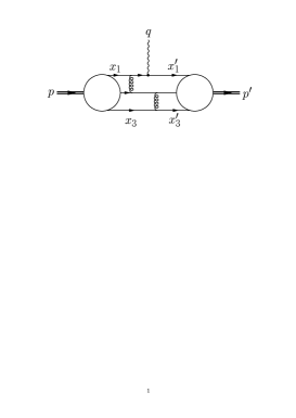
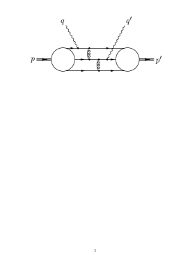
Figure 2: Sample Feyman graphs for form factors (left) and Compton scattering (right) within pQCD.

It turned out however that the leading-twist perturbative contributions to the proton form factor [8, 9] and to Compton scattering [10] are ways below experiment unless strongly asymmetric, i.e., end-point concentrated distribution amplitudes (DAs) are used. (A DA represents a LCWF integrated over tranverse momenta up to the factorisation scale.) The use of asymmetric DAs is however inconsistent since the bulk of a perturbative contribution evaluated from such a DA is accumulated in the end-point regions where the assumptions of perturbative calculations break down. It is also easy to see that a strongly asymmetric DA if combined with a Gaussian transverse momentum dependence in a LCWF

$$\Psi^{\lambda}_{N\beta}\propto\exp{\left[-a_{N}^{2}\sum^{N}_{i=1}k^{2}_{\perp i}/x_{i}\right]}\,,$$ (9)

leads to a large overlap contribution (evaluated by means of (6) and (4)) to the proton form factor exceeding the data by a factor of about 5 to 7 [8, 11]. Moreover, the ordinary parton distributions, evaluated from such LCWFs via (6) and (2) [8, 12], are in sharp disagreement with the results obtained from analyses of deep inelastic lepton-nucleon scattering [13]. A consistent description of form factors, parton distributions and, as we will see below, Compton scattering [2, 14, 15] which requires the inclusion of both the soft and the perturbative contributions, can only be achieved if DAs are used that are close to the asymptotic form $\Phi_{AS}=120x_{1}x_{2}x_{3}$. An example is given in [8] (see Fig. 3)

$$\Phi_{123}^{BK}=\Phi_{AS}\,\frac{1}{2}(1+3x_{1})$$ (10)

which refers to the $u_{+}u_{-}d_{+}$ configuration of the proton’s valence quarks. A recent instanton model study [16] seems to support the phenomenological DA (10). As remarked in [17] previous QCD sum rule studies [18] if restricted to the first order Appell polynomials, also provides a DA similar to the asymptotic one. The situation here seems to be quite analogous to the case of the pion where the analysis [19] of the CLEO data [20] on the $\pi\gamma$ transition form factor as well as the E791 measurement [21] clearly favour a form of the pion distribution amplitude that is close to the asymptotic one.

The perturbative contributions to the form factor and to Compton scattering evaluated from the DA (10) amounts to less than $10\%$ of experiment [8, 9, 10]. The onset of the perturbative regime is expected to lie above $t\simeq-100\,{\rm GeV}^{2}$. For wide-angle electroproduction of mesons there is no reliable perturbative result available as yet. On account of the experience with other exclusive reactions one may expect a small perturbative contribution here too. Only the decays $J/\Psi,\Psi^{\prime}\to p\bar{p}$ are dominated by perturbative physics [8, 22].

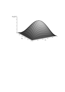
Figure 3: The DA (10) taken from Ref. [8] (left) and a typical Feynman diagram for hard electroproduction of mesons (right).

The crucial question now arises - how to calculate the soft contributions to wide-angle Compton scattering and electroproduction of mesons? The relevant handbag diagram for Compton scattering is shown in Fig. 1 and its generalization to electroproduction in Fig. 3 where a leading twist generation of the meson is assumed. Note that for the production of flavour neutral mesons active gluons have to be considered as well [23]. In Refs. [2, 23] the soft contributions to these processes are defined through the assumption that the (soft) LCWFs are dominated by parton virtualities $k_{i}^{2},k^{\prime}{}^{2}_{i}\raisebox{-3.0pt}{$\,\stackrel{{\scriptstyle\textstyle<}}{{\sim}}\,$}\Lambda^{2}$ and by intrinsic transverse momenta that satisfy $\tilde{k}^{2}_{\perp i}/\tilde{x}_{i},\>\hat{k}^{\prime}{}^{2}_{\perp i}/\hat{x}^{\prime}_{i}\raisebox{-3.0pt}{$\,\stackrel{{\scriptstyle\textstyle<}}{{\sim}}\,$}\Lambda^{2}$. One can then show that the active partons are approximately on-shell, collinear with their parent hadrons and they are carrying momentum fractions of about unity. Thus, the physical situation is that of a hard photon-parton scattering and a soft emission and re-absorption of partons by the protons. The amplitudes therefore factorise into subprocess amplitudes (either $\gamma^{*}q\to\gamma q$ or $\gamma^{*}q\to Mq$) and $1/\bar{x}$-moments of $\xi=0$ SPDs. The helicity amplitudes for Compton scattering, for instance, read [2]

$${\cal M}_{\mu^{\prime}+,\,\mu+}(s,t)\,=\,\;2\pi\alpha_{\rm em}\left[{\cal H}_{\mu^{\prime}+,\,\mu+}\,(R_{V}(t)+R_{A}(t))\,+\,{\cal H}_{\mu^{\prime}-,\,\mu-}\,(R_{V}(t)-R_{A}(t))\right]\,.$$ (11)

Proton helicity flip is neglected. The subprocess amplitudes ${\cal H}_{\mu^{\prime}\nu,\mu\nu}$ are calculated for massless quarks to lowest order perturbation theory [2, 23]. The soft form factors, $R_{V}$ and $R_{A}$, for an active quark of flavour $q$, are defined by

$$R_{V}^{\,q}(t)=\int_{-1}^{1}\frac{{\rm d}\bar{x}}{\bar{x}}\;H^{q}(\bar{x},0;t)\,,\qquad R_{A}^{\,q}(t)=\int_{-1}^{1}\frac{{\rm d}\bar{x}}{\bar{x}}\;\mbox{sign}(\bar{x})\,\widetilde{H}^{q}(\bar{x},0;t)\,.$$ (12)

The full form factors are specific to the process under consideration. All charged partons contribute to Compton scattering, (e.g. $R_{V}(t)=\sum e_{q}^{2}R_{V}^{q}(t)$) while in electroproduction the meson selects its valence quarks from the proton.

4 Results

In order to predict cross sections or polarization observables a model for the new form factors, $R_{V}$ and $R_{A}$, is required. Parameterizing the transverse momentum dependence of the LCWFs as in (9), which is in line with the central assumption of the soft physics approach of restricted $k^{2}_{\perp i}/x_{i}$, and using a common transverse size parameter ($a=a_{N}$) for simplicity, one can evaluate the $\xi=0$ SPDs from (6) and, without need for specifying the $x$-dependences of the LCWFs, relate the results to the ordinary parton distributions [2]

$$H^{q}(\bar{x},0;t)=\,\exp{\left[\,\frac{1}{2}\,a^{2}t\,\frac{1-\bar{x}}{\bar{x}}\right]}\,\;q(\bar{x})\,,\qquad\widetilde{H}^{q}(\bar{x},0;t)=\,\exp{\left[\,\frac{1}{2}\,a^{2}t\,\frac{1-\bar{x}}{\bar{x}}\right]}\,\Delta q(\bar{x})\,.$$ (13)

Taking the parton distributions from one of the current analyses of deep inelastic lepton-nucleon scattering, e.g., [13], using a value of 1 GeV^-1 for the transverse size parameter and evaluating the moments of the SPDs according to (4) and (12), one finds reasonable results in fair agreement with experiment [2, 14, 15]. Improvements are obtained by treating the lowest three Fock states explicitly with specified $x$-dependences, the DA (10) for the valence Fock state and similar ones for the next higher Fock states [2, 15]. The form factors $F_{1}$ and $R_{V}$, scaled by $t^{2}$, are displayed in Fig. 4. The scaled form factors exhibit broad maxima and, hence, mimic the dimensional counting rule behaviour in the $t$-range from about 5 to 15 GeV². This $t$-range is set by the transverse proton size. For very large momentum transfer the form factors turn gradually into the soft physics asymptotics $\sim 1/t^{4}$. This is the region where the perturbative contribution ($\sim 1/t^{2}$) takes the lead.

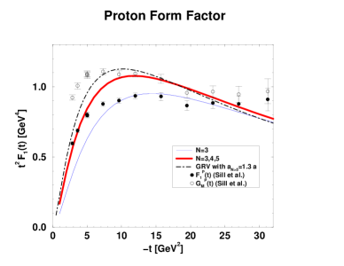
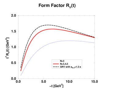
Figure 4: The Dirac (left) and the vector Compton (right) form factors of the proton as predicted by the soft physics approach [2, 8]. Data are taken from [24]. The data on the magnetic form factor, $G_{M}$, are shown in order to demonstrate the size of spin-flip effects.

The amplitude (11) leads to the real Compton cross section

$$\frac{{{\rm d}}\sigma}{{{\rm d}}t}=\frac{{{\rm d}}\hat{\sigma}}{{{\rm d}}t}\left[\,\frac{1}{2}(R_{V}^{2}(t)+R_{A}^{2}(t))-\,\frac{us}{s^{2}+u^{2}}\,(R_{V}^{2}(t)-R_{A}^{2}(t))\,\right]\,.$$ (14)

It is given by the Klein-Nishina cross section, ${{\rm d}}\hat{\sigma}/{{\rm d}}t$, multiplied by a factor that describes the structure of the nucleon in terms of two form factors. In view of the behaviour of the form factors (see Fig. 4) one infers from (14) that, in the soft physics approach, the Compton cross section approximately respects dimensional counting rule behaviour ($\propto s^{-6}$ at fixed cm scattering angle $\theta$) in a limited range of energy. The magnitude of the Compton cross section is fairly well predicted as is revealed by comparison with the admittedly old data [25] measured at rather low values of $s$, $-t$ and $-u$ (see Fig. 5). A cross section of similar magnitude has been obtained within the diquark model [26], a variant of the standard perturbative approach [7] in which diquarks are considered as quasi-elementary constituents of the proton. It seems difficult for the perturbative approach to account for the Compton data even if strongly aymmetric DAs are used [10]. Better data are needed for a crucial test of the soft physics approach and its confrontation with other approaches.

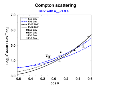
Figure 5: The Compton cross section, scaled by $s^{{}_{6}}$, (left) and the helicity correlation $A_{\rm LL}$ (right) as predicted by the soft physics approach [2, 15]. Data taken from [25].

The soft physics approach also predicts characteristic spin dependences of the Compton process. As an example predictions for the initial state helicity correlation

$$A_{\rm LL}\,\frac{{{\rm d}}\sigma}{{{\rm d}}t}=\frac{2\pi\alpha_{\rm em}^{2}}{s^{2}}\;R_{V}(t)R_{A}(t)\left(\frac{u}{s}-\frac{s}{u}\right)\,.$$ (15)

are shown in Fig. 5.

The cross sections for virtual Compton scattering have been calculated in [15]. Characteristic differences to the only other available results, namely those from the diquark model [26], are to be noticed. Thus, for instance, the beam asymmetry for $ep\to ep\gamma$ which is sensitive to the imaginary part of the longitudinal-transverse interference, is zero in the soft physics approach since all amplitudes are real. In the diquark model, on the other hand, this asymmetry is non-zero due to perturbatively generated phases of the Compton amplitudes. In regions of strong interference between the Compton and the Bethe-Heitler amplitudes the beam asymmetry is even spectacularly enhanced.

Along the same lines as Compton scattering wide-angle electroproduction of mesons has also been calculated [23]. As an example results for the $\rho^{0}$-production cross sections for longitudinally and transversally polarised photons are shown in Fig. 6. Similarly to deeply virtual electroproduction of mesons the longitudinal cross section dominates except for $Q^{2}\raisebox{-3.0pt}{$\,\stackrel{{\scriptstyle\textstyle<}}{{\sim}}\,$}1\,{\rm GeV}^{2}$. Contrary to a statement to be found in the literature occasionally the soft physics approach leads to a $s^{7}$-scaling of the cross sections provided $t/s$ and $Q^{2}/s$ are kept fixed and to the extent that the form factors $R^{M}_{V(A)}$ behave $\propto 1/t^{2}$. Unfortunately there is no wide-angle electroproduction data available as yet to compare with. For more details and predictions I refer to [23].

Figure 6: The transverse and longitudinal cross sections for the photoproduction of longitudinally polarised $\rho^{0}$ mesons at $s=40\,\,{\rm GeV}^{2}$ and a cm. scattering angle of $90^{\circ}$.

5 Summary

The SPDs, generalised PDFs, are new tools for the description of soft hadronic matrix elements. They are central elements which connect many different inclusive and exclusive processes: polarised and unpolarised PDFs are the $\zeta=t=0$ limits of SPDs, electromagnetic and Compton form factors represent moments of the SPDs, deeply virtual Compton scattering and hard meson electroproduction are controlled by them. A particularly interesting aspect is touched in exclusive reactions such as proton form factors and wide-angle Compton scattering. Their analysis by means of SPDs implies the calculation of soft physics contributions to these processes in which only one of the quarks is considered as active while the others act as spectators. The soft contributions formally represent power corrections to the asymptotically leading perturbative contributions in which all quarks participate in the subprocess. It seems that for momentum transfers around 10  GeV² the soft contribution dominates over the perturbative one. However, a severe confrontation of this approach with accurate data on wide-angle Compton scattering and electroproduction of mesons is pending.

References

- [1] D. Müller, D. Robaschik, B. Geyer, F. M. Dittes and J. Hořejši, Fortsch. Phys. 42 (1994) 101 [hep-ph/9812448]; X. Ji, Phys. Rev. D55 (1997) 7114 [hep-ph/9609381]; A. V. Radyushkin, Phys. Rev. D56 (1997) 5524 [hep-ph/9704207].
- [2] M. Diehl, T. Feldmann, R. Jakob and P. Kroll, Eur. Phys. J. C8 (1999) 409 [hep-ph/9811253].
- [3] M. Diehl, T. Feldmann, R. Jakob and P. Kroll, hep-ph/0009255, to be published in Nucl. Phys. B.
- [4] S. J. Brodsky, M. Diehl and D. S. Huang, hep-ph/0009254.
- [5] S. D. Drell and T. Yan, Phys. Rev. Lett. 24 (1970) 181.
- [6] B. Pire, J. Soffer and O. Teryaev, Eur. Phys. J. C8 (1999) 103 [hep-ph/9804284]; A. V. Radyushkin, Phys. Rev. D59 (1999) 014030 [hep-ph/9805342].
- [7] G.P. Lepage and S.J. Brodsky, Phys. Rev. D22, 2157 (1980).
- [8] J. Bolz and P. Kroll, Z. Phys. A356, 327 (1996).
- [9] J. Bolz et al., Z. Phys. C66 (1995) 267 [hep-ph/9405340]; B. Kundu et al., Eur. Phys. J. C8, 637 (1999) [hep-ph/9806419].
- [10] T. C. Brooks and L. Dixon, hep-ph/0004143; and private communication.
- [11] N. Isgur and C.H. Llewellyn Smith, Nucl. Phys. B317, 526 (1989).
- [12] A. Schäfer, L. Mankiewicz and Z. Dziembowski, Phys. Lett. B233, 217 (1989).
- [13] M. Glück, E. Reya and A. Vogt, Eur. Phys. J. C5 (1998) 461 [hep-ph/9806404].
- [14] A. V. Radyushkin, Phys. Rev. D58 (1998) 114008 [hep-ph/9803316].
- [15] M. Diehl, T. Feldmann, R. Jakob and P. Kroll, Phys. Lett. B460, 204 (1999) [hep-ph/9903268].
- [16] D. Diakonov and V. Y. Petrov, hep-ph/0009006.
- [17] V. Braun, R. J. Fries, N. Mahnke and E. Stein, hep-ph/0007279.
- [18] V. L. Chernyak, A. A. Ogloblin and I. R. Zhitnitsky, Z. Phys. C42, 583 (1989).
- [19] P. Kroll and M. Raulfs, Phys. Lett. B387, 848 (1996) [hep-ph/9605264]; T. Feldmann and P. Kroll, Eur. Phys. J. C5, 327 (1998) [hep-ph/9711231]; I. V. Musatov and A. V. Radyushkin, Phys. Rev. D56, 2713 (1997) [hep-ph/9702443].
- [20] J. Gronberg et al., CLEO collaboration Phys. Rev. D57, 33 (1998).
- [21] E. M. Aitala et al., E791 collaboration, hep-ex/0010043.
- [22] J. Bolz and P. Kroll, Eur. Phys. J. C2, 545 (1998) [hep-ph/9703252].
- [23] H. W. Huang and P. Kroll, Eur. Phys. J. C17, 423 (2000) [hep-ph/0005318].
- [24] A.F. Sill et al., Phys. Rev. D48, 29 (1993).
- [25] M.A. Shupe et al., Phys. Rev. D19, 1921 (1979).
- [26] P. Kroll, M. Schürmann and W. Schweiger, Intern. J. Mod. Phys. A6, 4107 (1991); P. Kroll, M. Schürmann and P.A.M. Guichon, Nucl. Phys. A598, 435 (1996).