Cosmic Birefringence within the Framework of Heterotic String Theory

Abstract

Low energy string theory predicts the existence of an axion field which can lead to cosmic birefringence. We solve the electromagnetic wave equations in the presence of such an axion and a dilaton field in order to determine their effect on the polarization of light. We find that the presence of dilaton field leads to a nontrivial modification of the final result. We comment on the possibility of discovering such an effect by observations of radio wave polarizations from distant radio galaxies and quasars. We have also determined the limits on the string theory parameters that are imposed by the current radio polarization data.

Pacs no. 14.80.Mz,98.80.Cq,11.25.-w,98.54.- h

I Introduction

There have been several studies which explore the possible existence of cosmic birefringence [1]. In recent work Kar et al [2] and Majumdar and Sengupta [3] has pointed out that the Kalb-Ramond field, which arises in supergravity theories, makes the space time birefringent. The authors solve the electromagnetic wave equations in the presence of such a field and predict that this field will lead to a redshift dependent rotation of polarization whose details depend on whether the universe is radiation or matter dominated. Earlier in Ref. [4] Carroll et al analyzed the polarizations of radio waves from distance galaxies and quasars as a function of redshifts and found no statistically significant effect. The observable of interest in that study was the angle $\beta=\chi-\psi$, where $\psi$ is the orientation angle of the axis of the radio galaxy and $\chi$ the observed polarization angle after the effect of Faraday rotation is taken out of the data. This can be done by making a straight line fit to the polarization angle $\theta(\lambda^{2})$ which can be expressed as

$$\theta(\lambda^{2})=RM\ \lambda^{2}+\chi$$ (1)

where $\lambda$ is the wavelength, $RM$ and $\chi$ are the slope and the intercept of the fit. $RM$ stands for rotation measure and depends on the plasma density and the parallel component of the background magnetic field along the direction of propagation of the wave. Later Ref. [5] claimed the existence of a large scale anisotropy in the same data. This claim was, however, questioned by many authors [6, 7, 8].

The possibility of local anisotropy, independent of redshift, was explored in Ref. [9] and earlier in [10, 11]. These authors found a statistically significant effect. The original claim made by Birch [10] in 1982 was dismissed by Bietenholz and Kronberg [12] in 1984 who compiled a larger data set which they claimed did not show any effect. However Jain and Ralston [9] argued that Ref. [12] did not pay careful attention to the parity of the correlation ansatz [13]. When the transformation properties of statistical distribution are taken into account the data does show a significant effect which is further enhanced by choosing an appropriate statistic as well as by putting some cuts on the data.

Inspite of the progress in our understanding in string theory in the last two decades, we are yet to have a string theory prediction that can be tested in the experiments. One of the main reason for such an unsatisfactory situation is that the energy scale at which stringy effects become significant is beyond the reach of present day experiments. It is thus believed that the most likely area for a confrontation between string theory and experiments is through extracting astrophysical or cosmological consequences of string theory which might be measurable today. With this kind of motivation in mind, we study in this paper the prediction of string theory for cosmic birefringence. However, as our knowledge of string theory is mostly perturbative in nature, we face several problems in carrying out such a study. These are mainly due to the presence of various massless moduli that are present in the low energy limit of string theory. We will point those out as we proceed.

Four dimensional heterotic string theory, in its low energy limit, contains moduli coming from compactification, gauge fields, dilaton and an axion. In this theory, coupling among various fields are unique and they are all controlled by the expectation value of dilaton. Given such a framework, we analyse the propagation of electromagnetic waves in curved metric background. Due to the presence of dilaton, as we will argue, medium turns into a conducting medium where the time variation of dilaton plays the role of effective conductivity. On the other hand, the axion rotates the plane of polarization of the electromagnetic wave causing non-trivial birefringence. However, notice that the dilaton (and other moduli) is a massless scalar in string theory. An important issue to resolve in string cosmology is to explain the absence of massless dilaton at the present time. One expects that a potential for dilaton will be generated in string theory through some non-perturbative effects and the dilaton will sit at the minimum of the potential picking up a mass. The mechanism of how precisely this should happen is still unknown in string theory. This, in turn, creates the most severe problem in comparing observational data with string theory. In the rest of the paper, we continue to treat dilaton as a massless scalar and find string prediction for cosmic birefringence. We hope that some of our results will be helpful when dilaton decoupling in string theory is properly understood. In general, we find that the relevant equations are hard to solve exactly. However, it is well-known that heterotic string theory in four dimensions is self dual. The duality group is parametrized by $SL(2,R)$ matrices. Using this property, in the next section, we generate some non-trivial solutions for various fields starting from some simple seed configuration. This, in turn, allows us to calculate birefringence of electromagnetic waves, propagating in radiation or matter dominated universe, in a fairly straightforward manner. However, since the solution generating technique does not saturate all possible allowed configurations, in section III, we solve the electromagnetic equations within the WKB approximation. We then discuss our results in section IV.

II Birefringence from Heterotic String

In the low energy limit, the heterotic string compactified on six-torus is represented by the following action [14]:

$$S = \int d^{4}x{\sqrt{-G}}e^{-\phi}\big{[}R_{G}+G^{\mu\nu}\partial_{\mu}\phi\partial_{\nu}\phi-{1\over{12}}H_{\mu\nu\rho}H^{\mu\nu\rho}~{}$$ (2)

$$- G^{\mu\rho}G^{\nu\lambda}F_{\mu\nu}^{(a)}(LML)_{ab}{F^{(b)}}_{\rho\lambda}+{1\over 8}G^{\mu\nu}{\rm Tr}(\partial_{\mu}ML\partial_{\nu}ML)\big{]}$$ (3)

where the gauge fields and the anti-symmetric three rank tensor field are defined as

$$F_{\mu\nu}^{(a)} = \partial_{\mu}A_{\nu}^{(a)}-\partial_{\nu}A_{\mu}^{(a)},$$ (4)

$$H_{\mu\nu\rho} = (\partial_{\mu}B_{\nu\rho}+2A_{\mu}^{(a)}L_{ab}F_{\nu\rho}^{(b)})+{\rm cyclic~{}permutations~{}of}~{}\mu,\nu,\rho.$$ (5)

The superscript $a$ on $F_{\mu\nu}$ runs from $1$ to $28$ denoting the $28$ gauge fields that appear in the four dimensional heterotic string action. Out of these $28$ gauge fields, $16$ are originally present in ten dimensions. The rest $12$ appear due to torus compactification. Among other terms in (3), $R_{G}$ is the scalar curvature associated with the metric $G_{\mu\nu}$ and $\phi$ is the dilaton. The $28\times 28$ dimensional matrix $M$ encodes all the scalars that appear due to compactification. In what follows, the detail of their structure will not be important. The matrix $L$ in (3) is also $28\times 28$ dimensional and is given by

$$L=\pmatrix{0&{I_{6}}&0\cr{I_{6}}&0&0\cr 0&0&{-I_{16}}\cr}$$ (6)

where $I_{n}$ denotes $n\times n$ identity matrix.

In the following, however, we will work with a truncated version of the effective action. We will turn off all the scalars that appear due to compactification. This essentially amounts to setting the matrix $M$ to identity. Furthermore, we will set all the gauge fields to zero except one. We will take this one to be present in the original ten dimensional heterotic action. We will see that this choice of trunctation makes the dynamics tractable and at the same time keeps the essential physics intact. In this approximation, the action, in the Einstein frame, reduces to

$$S=\int d^{4}x{\sqrt{-g}}[R_{g}-{1\over 2}g^{\mu\nu}\partial_{\mu}\phi\partial_{\nu}\phi-{1\over{12}}e^{-2\phi}H_{\mu\nu\rho}H^{\mu\nu\rho}-{e^{-\phi}}F_{\mu\nu}F^{\mu\nu}]$$ (7)

The equation of motion for the $B_{\mu\nu}$ following from the above action is

$$D_{\mu}(e^{-2\phi}H^{\mu\nu\rho})=0.$$ (8)

This, in turn, allows us to introduce a pseudoscalar field $\Psi$, known as axion, through the relation

$$H^{\mu\nu\rho}=-{1\over{\sqrt{-g}}}e^{2\phi}\epsilon^{\mu\nu\rho\sigma}\partial_{\sigma}\Psi.$$ (9)

With this definition of $\Psi$, the rest of the equations of motion are the following

$$R_{\mu\nu}={1\over 2}e^{2\phi}\partial_{\mu}\Psi\partial_{\nu}\Psi+2e^{-\phi}F_{\mu\rho}F_{\nu}^{\rho}-{1\over 2}g_{\mu\nu}e^{-\phi}F_{\rho\sigma}F^{\rho\sigma}+{1\over 2}\partial_{\mu}\phi\partial_{\nu}\phi,$$ (10)

$$D_{\mu}(e^{-\phi}F^{\mu\nu}+\Psi{\tilde{F}}^{\mu\nu})=0,$$ (11)

$$e^{2\phi}D^{\mu}D_{\mu}\Psi+2e^{2\phi}\partial_{\mu}\phi\partial^{\mu}\Psi-{\tilde{F}}_{\mu\nu}F^{\mu\nu}=0,$$ (12)

$$e^{2\phi}D^{\mu}D_{\mu}(e^{-\phi})+e^{3\phi}\partial_{\mu}\Psi\partial^{\mu}\Psi-e^{\phi}\partial_{\mu}\phi\partial^{\mu}\phi-F_{\mu\nu}F^{\mu\nu}=0.$$ (13)

Here

$${\tilde{F}}^{\mu\nu}={1\over{2{\sqrt{-g}}}}e^{\mu\nu\rho\sigma}F_{\rho\sigma},$$ (14)

which satisfies Bianchi identity

$$D_{\mu}{\tilde{F}}^{\mu\nu}=0.$$ (15)

It is easy to check that the set of equations (10)-(13) and (15) are invariant under the following set of $\rm{SL}(2,R)$ transformations [14]

$$\lambda\rightarrow\lambda^{\prime}={{a\lambda+b}\over{c\lambda+d}},~{}~{}F_{\mu\nu}\rightarrow F^{\prime}_{\mu\nu}=(c\Psi+d)F_{\mu\nu}-ce^{-\phi}{\tilde{F}}_{\mu\nu},~{}~{}g_{\mu\nu}\rightarrow g_{\mu\nu},$$ (16)

where $\lambda=\Psi+ie^{-\phi}$ and $a,~{}b,~{}c,~{}d$ are real parameters with $ad-bc=1$.

Here, in what follows, we will restrict ourselves to the case where dilaton, axion and the metric are only function of time. Our startegy will be to solve all the equations of motion in a fixed metric background. First, we take the metric as

$$ds^{2}=R^{2}{(\eta)}(-d\eta^{2}+dx^{2}+dy^{2}+dz^{2}).$$ (17)

The gauge field strength $F_{\mu\nu}$ in this background can be defined as [16]

$$F_{\mu\nu}=R^{2}(\eta)\pmatrix{0&{-E_{x}}&{-E_{y}}&{-E_{z}}\cr{E_{x}}&0&{B_{z}}&{-B_{y}}\cr{E_{y}}&{-B_{z}}&0&{B_{x}}\cr{E_{z}}&{B_{y}}&{-B_{x}}&0\cr}$$ (18)

With this definition, equation (11) reduces to

$$\nabla\cdot{\bf E}=0,~{}~{}\partial_{\eta}(e^{-\phi}{\bf E}R^{2})-\nabla\times(e^{-\phi}{\bf B}R^{2})=-2\partial_{\eta}\Psi{\bf B}R^{2}$$ (19)

Similarly the scalar equations are

$$\partial_{\eta}\partial^{\eta}\Psi-{2\over{R^{3}}}\partial_{\eta}R\partial_{\eta}\Psi-{2\over R^{2}}\partial_{\eta}\phi\partial_{\eta}\Psi+4R^{2}e^{-2\phi}{\bf E}\cdot{\bf B}=0,$$ (20)

$$\partial_{\eta}\partial^{\eta}\phi-{2\over{R^{3}}}\partial_{\eta}R\partial_{\eta}\phi+{e^{2\phi}\over{R^{2}}}(\partial_{\eta}\Psi)^{2}-2R^{2}e^{-\phi}(E^{2}-B^{2})=0.$$ (21)

On the otherhand, (15) reduces to

$$\nabla\cdot{\bf B}=0,~{}~{}\partial_{\eta}(R^{2}{\bf B})+\nabla\times(R^{2}{\bf E)}=0.$$ (22)

A Analyzing Equations in flat background

Before we go on to analyse more realistic scenario, it is worthwile to study (20) - (22) in flat metric background for which $R(\eta)=1$. Beside being completely tractable, this will indeed give us an idea of dilatonic and axionic influence on the propagation of electromagnetic waves. In this very special context, equations (20)-(22) reduce to the following forms:

$$\partial_{\eta}^{2}\Psi+2\partial_{\eta}\phi\partial_{\eta}\Psi=0,$$ (23)

$$\partial_{\eta}^{2}\phi-e^{2\phi}(\partial_{\eta}\Psi)^{2}+2e^{-\phi}({\bf E}^{2}-{\bf B}^{2})=0,$$ (24)

$$\partial_{\eta}(e^{-\phi}\partial_{\eta}{\bf B})-\nabla^{2}(e^{-\phi}{\bf B})=2\partial_{\eta}\Psi\nabla\times{\bf B}.$$ (25)

It is easy to check that when $\phi$ is turned of, the above equations reduce to the case analyzed in [2]. The very presence of dilaton $\phi$ effects the dynamics in a very crucial way. In order to understand the behaviour of the solutions, we first set the axion field $\Psi$ to zero. Then equation (25) reduces to

$$\partial_{\eta}^{2}{\bf B}-\partial_{\eta}\phi\partial_{\eta}{\bf B}-\nabla^{2}{\bf B}=0.$$ (26)

Such an equation for magnetic field is quite well known from the studies of electromagnetic wave propagation in conducting medium. As we can see from (26), the time variation of dilaton plays the role of effective conductivity of the medium. Such a damping factor, as usual, reduces the amplitude of the magnetic field $\bf B$.

The set of equations (22)-(25) are in general very hard to solve directly. Though it would be desirable to have such solutions, we would however use the property (16) of heterotic string theory to generate new solutions from some simple ones. To this end, we notice that if we set the dilaton field to zero (using sift symmetry of dilaton in heterotic string theory, we can always bring any constant dilaton field to zero), equations (22)-(25) possess a set of solutions [2]

$$\Psi=\int hdt=ht,~{}~{}~{}B_{\pm}(t,z)={b_{\pm}}e^{ikz}e^{i\omega_{\pm}t},~{}{\rm with}~{}{E}_{\pm}=\pm\frac{1}{k}\frac{d}{d\eta}(B_{\pm})=\pm{i\omega_{\pm}\over k}{B}_{\pm},$$ (27)

where $h$ is an integration constant and $\omega_{\pm}={\sqrt{k^{2}\pm 2hk}}$. In the above equations, we have defined ${\bf B}(t,z)={\bf b}(t)e^{ikz}$ with $z$ being the direction of propagation. Furthermore $b_{\pm}$ are defined as the circular polarization states, namely $b_{\pm}=b_{x}\pm ib_{y}$. Now writing $B_{\pm}=b_{\pm}e^{ikz}e^{i\varphi_{\pm}}$ and birefringence as $\delta\varphi={1\over 2}(\varphi_{+}-\varphi_{-})$, we get [2]

$$\delta\varphi=h(t_{2}-t_{1}),~{}{\rm for}~{}k>>h.$$ (28)

Here, for flat metric, $\eta$ is same as cosmic time $t$. Thus in the above equation, $t_{1}$ and $t_{2}$ are the earlier and present time.

As discussed earlier in (16), heterotic string theory in four dimension has self-duality symmetry. As a consequence, equations of motion for various fields are invariant under $SL(2,R)$ transformation. These transformations have the property to generate non-trivial field configurations from the known ones. A generic solution is thus parametrized by three independent parameters of $SL(2,R)$ group. Here, we start with the field configuration given in (27) where dilaton field is set to zero. Next, by the use of $SL(2,R)$ symmetry, we generate configurations with nontrivial dilaton and various other fields. Strictly following the transformation rules given in (16), and denoting the new configurations by $(\Psi^{\prime},\phi^{\prime},{\bf B}^{\prime},{\bf E}^{\prime})$, we, thus, get

$$\Psi^{\prime}={{ac\Psi^{2}+(bc+ad)\Psi+(ac+bd)}\over{(c\Psi+d)^{2}+c^{2}}},~{}~{}e^{-\phi^{\prime}}={1\over{(c\Psi+d)^{2}+c^{2}}}.$$ (29)

where $\Psi$ is given in (27). As expected the solutions are parametrized by three independent ${\rm SL}(2,R)$ parameters (taken here as) $b,c,d$. The other parameter $a$ is determined from the relation $ad-bc=1$. Furthermore, from the transformation property of $F_{\mu\nu}$ under $SL(2,R)$, we get

$${B}_{\pm}^{\prime}=[(c\Psi+d)\mp ic]b_{\pm}e^{ikz}e^{i\omega_{\pm}t}$$ (30)

$${E}_{\pm}^{\prime}=\pm{i\omega_{\pm}\over k}[(c\Psi+d)\mp ic]b_{\pm}e^{ikz}e^{i\omega_{\pm}t},~{}{\rm for}~{}k>>h$$ (31)

Thus the birefringence is then given by

$$\delta\varphi^{\prime}=h(t_{2}-t_{1})-\frac{1}{2}\left[\tan^{-1}\left(\frac{2(c\Psi+d)c}{(c\Psi+d)^{2}-c^{2}}\right)\right]_{t_{1}}^{t_{2}}\ \ \ \ ~{}{\rm for}~{}k>>h.$$ (32)

B Analyzing the equations in curved space

Here, we will study (11)-(15) for the general metric given in (17). We will follow the same strategy as the previous subsection in order to find solutions of equations of motion. Keeping this in mind, let us first consider (11)-(15) when the dilaton is set to zero. In that case, defining $F_{\pm}=R^{2}(\eta)B_{\pm}$, we get an equation for magnetic field as follows [2]:

$${d^{2}F_{\pm}\over{d\eta^{2}}}+(k^{2}\pm{2hk\over{R^{2}(\eta)}})F_{\pm}=0,$$ (33)

$$\Psi=h\int{1\over{R^{2}(\eta)}}d\eta,$$ (34)

with $h$ being a constant. If $R(\eta)$ increases fast enough with $\eta$ (which is indeed the case for radiation and matter dominated universe), a WKB type analysis will give us a very close to exact result for the above equation. Carrying out such a computation we get

$$F_{\pm}=f_{\pm}e^{ik\eta}e^{ikz}e^{\left[\pm i\int{{hd\eta}\over{R^{2}(\eta)}}\right]}=f_{\pm}e^{ik\eta}e^{ikz}e^{iS_{\pm}},$$ (35)

where we have $S_{\pm}=\pm\int{{hd\eta}\over R^{2}(\eta)}$. Like $B_{\pm}$ as in eqn.(24), one can also rewrite the eqn.(30) in the following way,

$$F_{\pm}=f_{\pm}e^{ikz}e^{i\omega_{\pm}^{R}\eta}$$ (36)

where, $\omega_{\pm}^{R}=\sqrt{(k^{2}\pm\frac{2hk}{R^{2}(\eta)})}$.

Now we have,

$$B_{\pm}={1\over{R^{2}(\eta)}}F_{\pm}={1\over{R^{2}(\eta)}}f_{\pm}e^{ik\eta}e^{ikz}e^{\pm i\int{{hd\eta}\over{R^{2}(\eta)}}},~{}~{}{\rm and}~{}~{}E_{\pm}=\pm{1\over{kR^{2}(\eta)}}{{d\over{d\eta}}(B_{\pm}R^{2}(\eta))}$$ (37)

From the above experssions for $B_{\pm}$, we see that the birefringence due to the presence of axion (dilaton is set to zero) is given by,

$$\delta\varphi=\frac{1}{2}(S_{+}-S_{-})=\int_{\eta_{1}}^{\eta_{2}}\frac{hd\eta}{R^{2}}=\int_{t_{1}}^{t_{2}}\frac{hdt}{R^{3}}$$ (38)

where we have converted the conformal time $(\eta)$ into cosmic time $t$ and $t_{1}$ and $t_{2}$ are the earlier time and present time respectively.

As before, starting from (34) and (37) and using the freedom of $SL(2,R)$ symmetry of equations of motion, we generate here large class of configurations, where axion and dilaton are given by

$$\Psi^{\prime}={{ac\Psi^{2}+(bc+ad)\Psi+(ac+bd)}\over{(c\Psi+d)^{2}+c^{2}}},~{}~{}e^{-\phi^{\prime}}={1\over{(c\Psi+d)^{2}+c^{2}}},$$ (39)

where $\Psi$ is given in (34). On the other hand, from the transformation property of $F_{{\mu}{\nu}}$ under $SL(2,R)$, we get

$$B^{\prime}_{\pm}=\left[(c\Psi+d)\mp ic(1\pm{h\over{kR^{2}(\eta)}})\right]B_{\pm}.$$ (40)

Consequently, the expression of birefringence is given by

$$\delta\varphi^{\prime}=-\frac{1}{2}\tan^{-1}\left[\frac{2(c\Psi+d)c}{(c\Psi+d)^{2}-c^{2}(1-\frac{h^{2}}{k^{2}R^{4}})}\right]+\int_{\eta_{1}}^{\eta_{2}}\frac{hd\eta}{R^{2}}$$ (41)

After having $\delta\varphi^{\prime}$ for general metric, let us concentrate on two particularly interesting cases; first radiation dominated case and then matter dominated case.

B1. Radiation dominated Universe: For radiation dominated universe, $R$ is given by $R(t)=R_{0R}t^{1/2}$, where $R_{0R}$ is a dimensionful constant. Instead of writing various fields explicitly in this particular case, we give the expression of birefringence that follows from (40). It is given by :

$$\delta\varphi^{\prime}=-\frac{1}{2}\tan^{-1}\left[\frac{2c(c\Psi+d)}{(c\Psi+d)^{2}-c^{2}(1-\frac{h^{2}}{k^{2}R_{0R}^{4}t_{2}^{2}})}\right]-\frac{h}{R_{0R}^{3}t_{2}}\left[1-(1+z)^{2}\right]\ .$$ (43)

B2. Matter dominated Universe: For matter dominated phase, $R$ is given by $R(t)=R_{0M}t^{2/3}$. In the same way as before, one can show that the birefringence is now given by:

$$\delta\varphi^{\prime}=-\frac{1}{2}\tan^{-1}\left[\frac{2c(c\Psi+d)}{(c\Psi+d)^{2}-c^{2}(1-\frac{h^{2}}{k^{2}R_{0M}^{4}(t_{2})^{8/3}})}\right]-\frac{h}{R_{0M}^{3}t_{2}}\left[1-(1+z)^{3/2}\right],$$ (44)

where, in both cases, the second term corresponds to the birefringence corresponding to zero dilaton field $\phi$. However, in both the cases, we see that the expression of $\delta\varphi^{\prime}$ depends on redshift $z$ in a crucial way. Furthermore, though very weak, $\delta\varphi^{\prime}$ has a dependence on the frequency $k$ of the electromagnetic wave.

III Approximate Solutions including the Dilaton Field

So far we have concentrated on solving the equations by first setting the dilaton field equal to zero and then using the $SL(2,R)$ transformation to generate solutions with nonzero dilaton field. However this procedure does not guarantee that all possible solutions to the equations are generated. We next solve the field equations directly within the WKB approximation. We first write the electromagnetic field equation in terms of the variable $S_{\pm}$. Since $S_{\pm}$ is assumed to be a slowly varying function we drop its second derivatives and terms proportional to $[S^{\prime}_{\pm}]^{2}$. With these approximations the field equations reduce to

$${\partial S_{\pm}^{R}\over\partial t} = \mp{\partial\psi\over\partial t}e^{\phi}$$ (45)

$${\partial\psi\over\partial t} = {h\over R^{3}}e^{-2\phi}$$ (46)

$${\partial^{2}\phi\over\partial t^{2}} = -{3\over R}{\partial R\over\partial t}{\partial\phi\over\partial t}+{h^{2}\over R^{6}}e^{-2\phi}$$ (47)

$$S^{I}_{\pm} = -\phi/2$$ (48)

where $S_{\pm}^{R}$ and $S_{\pm}^{I}$ are the real and imaginary parts of the function $S_{\pm}$. We also drop the term proportional to $h^{2}$ in the dilaton field equation (47) since it is higher order in $h$ and hence expected to give negligible contribution. We then find that Eq. 47 can be solved to give

$$\phi=B+A/t$$

where $A$ and $B$ are constants. Furthermore, $S_{\pm}^{R}$ are given by,

$$S^{R}_{\pm}=\mp{he^{-B}\over AR_{0M}^{3}}e^{-A/t_{2}}\left[1-\exp\left(-{A\over t_{2}}\left((1+z)^{3/2}-1\right)\right)\right]$$ (49)

The rotation in polarization is given by $\delta\phi=(S_{+}-S_{-})/2$. The functional form of the rotation angle is plotted in Fig. 1 as a function of redshift for some arbitrary choice of the parameters $\zeta=-e^{-A/t_{2}}he^{-B}/AR_{0M}^{3}$ and $\xi=A/t_{2}$. Hence we find that the dilaton field leads to a nontrivial change in the redshift dependence of the rotation in polarization. Whereas in the absence of dilaton we predict a steady increase of the polarization rotation angle with redshift, in the present case the rotation turns on only at large redshifts.

FIG. 1.: The redshift dependence of the polarization angle for some representative values of the parameters $\zeta$ and $\xi$

We next consider the polarization data from distant quasars and radio galaxies in order to determine if there exists a signal of the type predicted by our analysis. We considered all the sources that were used in the statistical analysis in Ref. [9] for which the information about redshift was available. The NASA extragalactic data base (NED) was used to update the information about redshifts. We compiled a total of 231 sources in this manner. We also examined the data after removing all sources which lie within $\pm 30^{o}$ of the galactic plane. This cut is useful since it removes many sources with very large rotation measures and hence reduces the possibility of bias in data. The bias in rotation measure can arise due to the $n\pi$ ambiquity in the measurement of linear polarization. After imposing this cut on the data we are left with a total of 160 sources. We use the maximum likelihood analysis in order to determine the presence of correlation in data. For the null hypothesis we use the von Mises (vM) distribution which serves as a prototype for the statistical fluctuations for circular data. It is given by [17],

$$f_{\rm vM}(\beta)={\exp\left[\kappa\cos 2(\beta-\overline{\beta})\right]\over\pi I_{0}(\kappa)}$$ (50)

where $\kappa$ is a parameter which measures the concentration of the population, $\beta$ is the angle between the axis of the radio galaxy and the observed polarization after taking out the effect of Faraday rotation and $\overline{\beta}$ is the mean angle. The factor 2 has been inserted since the polarization angle is ambiguous by $n\pi$ and not $2n\pi$ [13]. The distribution peaks very close to $\overline{\beta}=\pi/2$ and therefore it is reasonable to eliminate this parameter by setting it exactly equal to $\pi/2$ [9]. We are therefore left with only one free parameter and the fit to the entire data set leads to $\kappa=0.67$ and after the galactic cut we find $\kappa=0.71$.

                  
                  

FIG. 2.: The distribution of the offset angle $\beta$ between the intrinsic polarization $\chi$ and the orientation axis of the radio galaxy $\psi$ for (a) full data containing 231 points and (b) after putting the cut on redshift, $z>0.5$.

We next study the redshift, $z$, dependence of distribution. It turns out that the distribution has a strong dependence on the redshift which can be modelled by the following generalization of the vM distribution,

$$F(\beta,z)=N(\kappa,\kappa_{1}){\exp\left[-(\kappa+\kappa_{1}z)\cos(2\beta)\right]}$$ (51)

where $N(\kappa,\kappa_{1})$ is a normalization factor. Maximizing the likelihood in this case gives $\kappa=0.29$ and $\kappa_{1}=0.90$. The maximum likelihood increases by 7 units, i.e. $L_{II}-L_{I}=T=7$, where $L_{I}$ and $L_{II}$ are the maximum likelihoods for the distributions given in equations (50) and (51) respectively. After making the galactic cut the corresponding parameters are $\kappa=0.32$, $\kappa_{1}=0.97$ and $T=5.1$. The statistic $2T$ is distributed as $\chi^{2}_{1}$. The increase in the maximum likelihood is quite large and implies that the width of the distribution has significant dependence on the redshift. This is also apparent from a plot of the distribution of the angle $2\beta$ shown in Fig. 2 for the complete data set and after imposing the cut on redshift, $z>0.5$. We find that after imposing the cut the distribution is more strongly peaked at $\beta=\pi/2$.

In order to search for a correlation of the type implied by Eq. 49 we propose the following distribution

$$G(\beta,z)=N(\kappa,\kappa_{1},\zeta,\xi){\exp\left[-(\kappa+\kappa_{1}z)\cos(2\beta)+p(z,\zeta,\xi)\sin(2\beta)\right]}$$ (52)

where $N(\kappa,\kappa_{1},\zeta,\xi)$ is a normalization factor and $p(z,\zeta,\xi)$ is given by

$$p(z,\zeta,\xi)=\zeta\left[1-\exp\left(\xi\left((1+z)^{3/2}-1\right)\right)\right]$$ (53)

This form of the distribution will lead to the relationship (49) for the polarization angle $<\beta(z)>$, where $<>$ denotes the mean value, as long as deviation of $<\beta>$ from $\pi/2$ is small.

The best fit parameters for the correlated ansatz are $\kappa=0.27,\ \kappa_{1}=0.98,\ \zeta=8.0\times 10^{-14},\ \xi=7.1$ with the statistic $2T=2(L_{III}-L_{II})=5.34$ for the full data set and $\kappa=0.28,\ \kappa_{1}=1.1,\ \zeta=8.8\times 10^{-8},\ \xi=4.1$ with the statistic $2T=6.9$ for the case of galactic cut. Here $L_{III}$ is the maximum likelihood for the distribution given in equation (52). The corresponding percentage values (p-values) for these two cases, with and without the galactic cut, are 7% and 3.5% respectively. These p-values represent the probabilities that the correlation seen in data can be obtained from a statistical fluctuation. After making the galactic cut the results correspond to a $2\sigma$ effect. Hence these results show marginal statistical significance. Although they show a significant correlation it is clear from the best fit parameters that the solution prefers the extreme values of the parameter $\zeta$ very close to zero. This implies that the deviation of $\beta$ from $\pi/2$ is very close to zero for a wide range of redshifts and deviates from zero only for relatively large redshifts. This is clearly seen in Fig. 3 where we plot the data and our best fit model for the case of galactic cut. On the y-axis we plot the $\sin 2\beta$ in order to deal with quantities invariant under angular coordinate transformations. The data, $\sin 2\beta$, has been averaged over the redshift interval of 0.25 in order to reduce the noise. The number of data points in each bin, starting from the smallest redshift, are 54,19,15,13,10,9,9,11,7,4,3,2,2,1,1 respectively.

FIG. 3.: The fit to the polarization offset angle $\beta$ for distant radio galaxies and quasars. The redshift is plotted on the x-axis and the mean (over a redshift interval of 0.25) of $\sin(2\beta)$ is plotted on the y-axis. The region within $\pm 30^{o}$ of the galactic plane was eliminated from the data.

If we eliminate the two largest redshift points then we do not see any significant effect. Strictly speaking we were unable to find the maxima of the likelihood. The fit was driven to ridicuously large values of $\xi>100$ and we did not search beyond these extreme values. The statistic $2T$ in this case was roughly $1.6$ which has p-values of 45% and hence shows no significant correlation. In Fig. 4 we show the limits of the parameters $\zeta$ and $\xi$ that are imposed by the polarization data. The limits are obtained by excluding all sources which lie within $\pm 30^{o}$ from the galactic plane. However the results remain unchanged even if this cut is not imposed.

                  

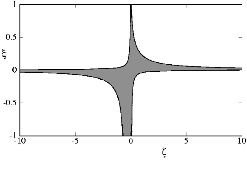
FIG. 4.: Limits on the values of the parameters $\zeta$ and $\xi$ from the polarization data from distant quasars and radio galaxies after eliminating all sources which lie within $\pm 30^{o}$ from the galactic plane. The results do not change appreciably if this cut is not imposed. The shaded region represents the allowed range of these parameters. The two largest redshift points were deleted for this analysis.

IV Conclusions

In this paper, we have studied cosmic birefringence in the framework of perturbative four-dimensional heterotic string theory. Due to coupling between dilaton and axion in this theory, we have shown that the dilaton field changes the birefringence produced by the axion field in a nontrivial way. We obtained an approximate expression for the rotation in polarization predicted by heterotic string theory within the WKB approximation. We analysed the data for distant quasars and radio galaxies to determine if the effect is present in the data. We find a marginally significant effect. However the correlation is caused primarily by two largest redshift points and the effect is lost after these points are eliminated. Hence we find that the data does not show significant correlation but the large redshift points are suggestive that a signal might exist. This should be thoroughly investigated by accummulating more data at the largest redshifts. We have also determined the limits on the string theory parameters that are imposed by the current polarization data from distant quasars and radio galaxies.

We, furthermore, like to point out that all these calculations were done taking dilaton as a massless scalar. As explained in the introduction, one of the biggest problem in string theory is to find a mechanism to remove this massless dilaton from present day physics. One expects that a potential for dilaton will be generated in string theory through some non-perturbative effects and the dilaton will sit at the minimum of the potential picking up a mass. As the mecanism of how precisely this should happen is still not clear in string theory, we have not dealt with such a scenario in this paper.

Acknowledgements: PJ thanks John Ralston for very useful discussions and for providing very useful insights into the statistical analysis of this data. This research has made use of the NASA/IPAC Extragalactic Database (NED) which is operated by the Jet Propulsion Laboratory, California Institute of Technology, under contract with the National Aeronautics and Space Administration.

REFERENCES

- [1] W.-T. Ni, Phys. Rev. Lett. 38, 301 (1977); R. B. Mann and J. W. Moffat, Can. J. Phys. 59 1730 (1981); M. Sachs, General Relativity and Matter (Reidel, 1982); P. Sikivie, Phys. Lett. B137, 353 (1984); P. Sikivie, Phys. Rev. D 32 1560, (1985); C. Wolf, Phys. Lett. A132, 151 (1988), A 145, 413 (1990); R. B. Mann, J. W. Moffat, and J. H. Palmer, ibid 62, 2765 (1989); C. M. Will, Phys. Rev. Lett. 62, 369 (1989); D. Harari and P. Sikivie, Phys. Lett. B 289, 67 (1992); D. V. Ahluwalia and T. Goldman, Mod. Phys. Lett. A28, 2623 (1993); J. P. Ralston, Phys. Rev. D 51, 2018 (1995). M. Sachs, Nuovo Cimento 111A, 611 (1997);
- [2] S. Kar, P. Majumdar, S. Sengupta and A. Sinha, gr-qc/0006097.
- [3] P. Majumdar and S. Sengupta, Class. Quant. Grav. 16, L89 (1999).
- [4] S. M. Carroll, G. B. Field and R. Jackiw, Phys. Rev. D 41, 1231 (1990).
- [5] B. Nodland and J. P. Ralston, Physical Review Letters 78, 3043 (1997).
- [6] D. J. Eisenstein and E. F. Bunn, Phys. Rev. Lett. (Comments) 79, 1957.
- [7] S. M. Carroll and G. B. Field, Phys. Rev. Lett. 79, 2934 (1997).
- [8] T. J. Loredo, E. E. Flanagan, and I. M. Wasserman, Phys. Rev. D 56, 7057 (1997).
- [9] P. Jain and J. P. Ralston, Mod. Phys. Lett. A14, 417 (1999).
- [10] P. Birch, Nature, 298, 451 (1982)
- [11] D. G. Kendall and A. G. Young, MNRAS, 207, 637 (1984).
- [12] M. F. Bietenholz and P. P. Kronberg, ApJ, 287, L1-L2 (1984).
- [13] J. P. Ralston and P. Jain, International Journal of Modern Physics D 8, 537 (1999).
- [14] A. Sen, Int. Jour. Mod. Phys. A9, 3703 (1994).
- [15] R.D. Reasenberg, I.I. Shapiro, P.E. MacNeil, R.B. Goldstein, J.C. Breidenthal, J.P. Brenkle, D.L. Cain, T.M. Kaufman, T.A. Komarek and A.I. Zygielbaum, Astrophys. J. Lett. 234, L219 (1979).
- [16] S. M. Carroll and G. B. Field, Phys. Rev. D 43, 3789 (1991).
- [17] N. I. Fisher, Statistics of Circular Data, (Cambridge, 1993).