Lectures on Technicolor and Compositeness

Abstract

Lecture 1 provides an introduction to dynamical electroweak symmetry breaking. Lectures 2 and 3 give an introduction to compositeness, with emphasis on effective lagrangians, power-counting, and the ’t Hooft anomaly-matching conditions.

Lecture 1: Technicolor

1 Dynamical Electroweak Symmetry Breaking

The simplest theory of dynamical electroweak symmetry breaking is technicolor.[3, 4] Consider an $SU(N_{TC})$ gauge theory with fermions in the fundamental representation of the gauge group

$$\Psi_{L}=\left(\begin{array}[]{c}U\\ D\end{array}\right)_{L}\,\,\,\,\,\,\,\,U_{R},D_{R}~{}.$$ (1)

The fermion kinetic energy terms for this theory are

$${\cal L} = \bar{U}_{L}i\hbox to0.0pt{\hbox to8.55695pt{\hfil/\hfil}\hss}DU_{L}+\bar{U}_{R}i\hbox to0.0pt{\hbox to8.55695pt{\hfil/\hfil}\hss}DU_{R}+$$

$$\bar{D}_{L}i\hbox to0.0pt{\hbox to8.55695pt{\hfil/\hfil}\hss}DD_{L}+\bar{D}_{R}i\hbox to0.0pt{\hbox to8.55695pt{\hfil/\hfil}\hss}DD_{R}~{},$$

and, like QCD in the $m_{u}$, $m_{d}\to 0$ limit, they have a chiral $SU(2)_{L}\times SU(2)_{R}$ symmetry.

As in QCD, exchange of technigluons in the spin zero, isospin zero channel is attractive, causing the formation of a condensate

$${\lower 15.0pt\hbox{ \epsfbox{figures/qqbar.ps}}\ \ \rightarrow\ \ \langle\bar{U}_{L}U_{R}\rangle=\langle\bar{D}_{L}D_{R}\rangle\neq 0\,,}$$ (3)

which dynamically breaks $SU(2)_{L}\times SU(2)_{R}\to SU(2)_{V}$. These broken chiral symmetries imply the existence of three massless Goldstone bosons, the analogs of the pions in QCD.

Now consider gauging $SU(2)_{W}\times U(1)_{Y}$ with the left-handed fermions transforming as weak doublets and the right-handed ones as weak singlets. To avoid gauge anomalies, in this one-doublet technicolor model we will take the left-handed technifermions to have hypercharge zero and the right-handed up- and down-technifermions to have hypercharge $\pm 1/2$. The spontaneous breaking of the chiral symmetry breaks the weak-interactions down to electromagnetism. The would-be Goldstone bosons become the longitudinal components of the $W$ and $Z$

$$\pi^{\pm},\,\pi^{0}\,\rightarrow\,W^{\pm}_{L},\,Z_{L}~{},$$ (4)

which acquire a mass

$$M_{W}={gF_{TC}\over 2}~{}.$$ (5)

Here $F_{TC}$ is the analog of $f_{\pi}$ in QCD. In order to obtain the experimentally observed masses, we must have $F_{TC}\approx 246{\rm GeV}$ and hence this model is essentially QCD scaled up by a factor of

$${F_{TC}\over f_{\pi}}\approx 2500\,.$$ (6)

While I have described only the simplest model above, it is straightforward to generalize to other cases. Any strongly interacting gauge theory with a chiral symmetry breaking pattern $G\to H$, in which $G$ contains $SU(2)_{W}\times U(1)_{Y}$ and subgroup $H$ contains $U(1)_{em}$ (but not $SU(2)_{W}\times U(1)_{Y}$) will break the weak interactions down to electromagnetism. In order to be consistent with experimental results, however, we must also require that $H$ contain custodial[5, 6] $SU(2)_{V}$. This custodial symmetry insures that the $F$-constant associated with the $W^{\pm}$ and $Z$ are equal and therefore that the relation

$$\rho={M^{2}_{W}\over M^{2}_{Z}\cos^{2}\theta_{W}}=1$$ (7)

is satisfied at tree-level. If the chiral symmetry is larger than $SU(2)_{L}\times SU(2)_{R}$, theories of this sort will contain additional (pseudo-) Goldstone bosons which are not “eaten” by the $W$ and $Z$.

2 Flavor Symmetry Breaking and ETC

2.1 Fermion Masses & ETC Interactions

In order to give rise to masses for the ordinary quarks and leptons, we must introduce interactions which connect the chiral-symmetries of technifermions to those of the ordinary fermions. The most popular choice[7, 8] is to introduce new broken gauge interactions, called extended technicolor interactions (ETC), which couple technifermions to ordinary fermions. At energies low compared to the ETC gauge-boson mass, $M_{ETC}$, these effects can be treated as local four-fermion interactions

$${\lower 15.0pt\hbox{\epsfbox{figures/etc.eps}}}\ \ \rightarrow\ \ {{g_{ETC}^{2}\over M^{2}_{ETC}}}(\overline{\Psi}_{L}U_{R})({\overline{q}_{R}q_{L}})~{}.$$ (8)

After technicolor chiral-symmetry breaking and the formation of a $\langle\bar{U}U\rangle$ condensate, such an interaction gives rise to a mass for an ordinary fermion

$$m_{q}\approx{{g_{ETC}^{2}\over M^{2}_{ETC}}}\langle\overline{U}U\rangle_{ETC}~{},$$ (9)

where $\langle\overline{U}U\rangle_{ETC}$ is the value of the technifermion condensate evaluated at the ETC scale (of order $M_{ETC}$). The condensate renormalized at the ETC scale in eq. (9) can be related to the condensate renormalized at the technicolor scale as follows

$$\langle\overline{U}U\rangle_{ETC}=\langle\overline{U}U\rangle_{TC}\exp\left(\int_{\Lambda_{TC}}^{M_{ETC}}{d\mu\over\mu}\gamma_{m}(\mu)\right)~{},$$ (10)

where $\gamma_{m}(\mu)$ is the anomalous dimension of the fermion mass operator and $\Lambda_{TC}$ is the analog of $\Lambda_{QCD}$ for the technicolor interactions.

For QCD-like technicolor (or any theory which is “precociously” asymptotically free), $\gamma_{m}$ is small in the range between $\Lambda_{TC}$ and $M_{ETC}$. Using dimensional analysis [9, 10, 11, 12] we find

$$\langle\overline{U}U\rangle_{ETC}\approx\langle\overline{U}U\rangle_{TC}\approx 4\pi F^{3}_{TC}~{}.$$ (11)

In this case eq. (9) implies that

$${{M_{ETC}\over g_{ETC}}}\approx 40{\rm\,TeV}\left({F_{TC}\over 250{\rm\,GeV}}\right)^{3\over 2}\left({100{\rm\,MeV}\over m_{q}}\right)^{1\over 2}~{}.$$ (12)

In order to orient our thinking, it is instructive to consider a simple “toy” extended technicolor model. The model is based on an $SU(N_{ETC})$ gauge group, with technicolor as an extension of flavor. In this case $N_{ETC}=N_{TC}+N_{F}$, and the model contains the (anomaly-free) set of fermions

$$\begin{array}[]{l@{\extracolsep{15pt}}l}Q_{L}=(N_{ETC},3,2)_{1/6}&L_{L}=(N_{ETC},1,2)_{-1/2}\\ U_{R}=(N_{ETC},3,1)_{2/3}&E_{R}=(N_{ETC},1,1)_{-1}\\ D_{R}=(N_{ETC},3,1)_{-1/3}&N_{R}=(N_{ETC},1,1)_{0}~{},\end{array}$$ (13)

where we display their quantum numbers under $SU(N_{ETC})\times SU(3)_{C}\times SU(2)_{W}\times U(1)_{Y}$. We break the ETC group down to technicolor in three stages

$SU(N_{TC}+3)$

$\Lambda_{1}\ \ \ \ \ \downarrow\ \ \ \ \ m_{1}\approx{4\pi F^{3}\over\Lambda^{2}_{1}}$

$SU(N_{TC}+2)$

$\Lambda_{2}\ \ \ \ \ \downarrow\ \ \ \ \ m_{2}\approx{4\pi F^{3}\over\Lambda^{2}_{2}}$

$SU(N_{TC}+1)$

$\Lambda_{3}\ \ \ \ \ \downarrow\ \ \ \ \ m_{3}\approx{4\pi F^{3}\over\Lambda^{2}_{3}}$

$SU(N_{TC})$

resulting in three isospin-symmetric families of degenerate quarks and leptons, with $m_{1}<m_{2}<m_{3}$. Note that the heaviest family is related to the lightest ETC scale!

Before continuing our general discussion, it is worth noting a couple of points. First, in this example the ETC gauge bosons do not carry color or weak charge

$$[G_{ETC},SU(3)_{C}]=[G_{ETC},SU(2)_{W}]=0~{}.$$ (14)

Furthermore, in this model there is one technifermion for each type of ordinary fermion: that is, this is a “one-family” technicolor model.[13] Since there are eight left- and right- handed technifermions, the chiral symmetry of the technicolor theory is (in the limit of zero QCD and weak couplings) $SU(8)_{L}\times SU(8)_{R}\to SU(8)_{V}$. Such a theory would yield $8^{2}-1=63$ (pseudo-) Goldstone bosons. Three of these Goldstone bosons are unphysical — the corresponding degrees of freedom become the longitudinal components of the $W^{\pm}$ and $Z$ by the Higgs mechanism. The remaining 60 must somehow obtain a mass. This will lead to the condition in eq. (14) being modified in a realistic model.[7] We will return to the issue of pseudo-Goldstone bosons below.

The most important feature of this or any ETC-model is that a successful extended technicolor model will provide a dynamical theory of flavor! As in the toy model described above and as explicitly shown in eq. (8) above, the masses of the ordinary fermions are related to the masses and couplings of the ETC gauge-bosons. A successful and complete ETC theory would predict these quantities and, hence, the ordinary fermion masses.

Needless to say, constructing such a theory is very difficult. No complete and successful theory has been proposed. Examining our toy model, we immediately see a number of shortcomings of this model that will have to be addressed in a more realistic theory:

• What breaks ETC?

• Do we require a separate scale for each family?

• How do the $T_{3}=\pm{1\over 2}$ fermions of a given generation receive different masses?

• How do we obtain quark mixing angles?

• What about right-handed technineutrinos and $m_{\nu}$?

2.2 Flavor-Changing Neutral-Currents

Perhaps the single biggest obstacle to constructing a realistic ETC model (or any dynamical theory of flavor) is the potential for flavor-changing neutral currents.[7] Quark mixing implies transitions between different generations: $q\to\Psi\to q^{\prime}$, where $q$ and $q^{\prime}$ are quarks of the same charge from different generations and $\Psi$ is a technifermion. Consider the commutator of two ETC gauge currents:

$$[\overline{q}\gamma\Psi,\overline{\Psi}\gamma q^{\prime}]\,\supset\,\overline{q}\gamma q^{\prime}\,.$$ (15)

Hence we expect there are ETC gauge bosons which couple to flavor-changing neutral currents. In fact, this argument is slightly too slick: the same applies to the charged-current weak interactions! However in that case the gauge interactions, $SU(2)_{W}$, respect a global $(SU(3)\times U(1))^{5}$ chiral symmetry leading to the usual GIM mechanism.

Unfortunately, the ETC interactions cannot respect the same global symmetry; they must distinguish between the various generations in order to give rise to the masses of the different generations. Therefore, flavor-changing neutral-current interactions are (at least at some level) unavoidable.

The most severe constraints come from possible $|\Delta S|=2$ interactions which contribute to the $K_{L}$-$K_{S}$ mass difference. In particular, we would expect that in order to produce Cabibbo-mixing the same interactions which give rise to the $s$-quark mass could cause the flavor-changing interaction

$${\cal L}_{|\Delta S|=2}={g^{2}_{ETC}\,\theta^{2}_{sd}\over{M^{2}_{ETC}}}\,\,\left(\overline{s}\Gamma^{\mu}d\right)\,\,\left(\overline{s}\Gamma^{\prime}_{\mu}d\right)+{\rm h.c.}~{},$$ (16)

where $\theta_{sd}$ is of order the Cabibbo angle. Such an interaction contributes to the neutral kaon mass splitting

$$(\Delta M^{2}_{K})_{ETC}={g^{2}_{ETC}\,\theta^{2}_{sd}\over{M^{2}_{ETC}}}\,\langle\overline{K^{0}}|\overline{s}\Gamma^{\mu}d\,\overline{s}\Gamma^{\prime}_{\mu}d|K^{0}\rangle+{\rm c.c.}$$ (17)

Using the vacuum insertion approximation we find

$$(\Delta M^{2}_{K})_{ETC}\simeq{g^{2}_{ETC}\,{\rm Re}(\theta^{2}_{sd})\over{2M^{2}_{ETC}}}\,f^{2}_{K}M^{2}_{K}~{}.$$ (18)

Experimentally[2] we know that $\Delta M_{K}<3.5\times 10^{-12}\,{\rm\,MeV}$ and, hence, that

$${M_{ETC}\over{g_{ETC}\,\sqrt{{\rm Re}(\theta^{2}_{sd})}}}>600\,{\rm\,TeV}$$ (19)

Using eq. (9) we find that

$$m_{q,\ell}\simeq{g_{ETC}^{2}\over{M_{ETC}^{2}}}\langle\overline{T}T\rangle_{ETC}<{0.5\,{\rm\,MeV}\over{N_{D}^{3/2}\,\theta_{sd}^{2}}}\,$$ (20)

showing that it will be difficult to produce the $s$-quark mass, let alone the $c$-quark!

2.3 Pseudo-Goldstone Bosons

A “realistic” ETC theory may require a technicolor sector with a chiral symmetry structure bigger than the $SU(2)_{L}\times SU(2)_{R}$ discussed initially. The prototypical theory has one-family of technifermions, as incorporated in our toy model. As discussed there, the theory has an $SU(8)_{L}\times SU(8)_{R}\to SU(8)_{V}$ chiral symmetry breaking structure resulting in 63 Goldstone bosons, 3 of which are unphysical. The quantum numbers of the 60 remaining Goldstone bosons are shown in table 1. Clearly, these objects cannot be massless in a realistic theory!

SU$(3)_{C}$	SU$(2)_{V}$	Particle
$1$	$1$	$P^{0\prime}\;,\;\omega_{T}$
$1$	$3$	$P^{0,\pm}\;,\;\rho^{0,\pm}_{T}$
$3$	$1$	$P^{0\prime}_{3}\;,\;\rho^{0\prime}_{T3}$
$3$	$3$	$P^{0,\pm}_{3}\;,\;\rho^{0,\pm}_{T3}$
$8$	$1$	$P^{0\prime}_{8}(\eta_{T})\;,\;\rho^{0\prime}_{T8}$
$8$	$3$	$P^{0,\pm}_{8}\;,\;\rho^{0,\pm}_{T8}$

Table 1: Quantum numbers of the 60 physical Goldstone bosons (and the corresponding vector mesons) in a one-family technicolor model. Note that the mesons that transform as 3’s of QCD are complex fields.

In fact, the ordinary gauge interactions break the full $SU(8)_{L}\times SU(8)_{R}$ chiral symmetry explicitly. The largest effects are due to QCD, and the color octets and triplets mesons get masses of order 200 – 300 GeV, in analogy to the electromagnetic mass splitting $m_{\pi^{+}}-m_{\pi^{0}}$ in QCD. Unfortunately, the others[7] are massless to O($\alpha$)!

Luckily, the ETC interactions (which we introduced in order to give masses to the ordinary fermions) are capable of explicitly breaking the unwanted chiral symmetries and producing masses for these mesons. This is because in addition to coupling technifermions to ordinary fermions, some ETC interactions also couple technifermions to one another.[7] Using Dashen’s formula,[15] we can estimate that such an interaction can give rise to an effect of order

$$F^{2}_{TC}M^{2}_{\pi_{T}}\propto{g^{2}_{ETC}\over M^{2}_{ETC}}\langle(\overline{T}T)^{2}\rangle_{ETC}~{}.$$ (21)

In the vacuum insertion approximation for a theory with small $\gamma_{m}$, we may rewrite the above formula using eq. (9) and find that

$$M_{\pi_{T}}\simeq 55{\rm\,GeV}\sqrt{m_{f}\over 1{\rm\,GeV}}\sqrt{250{\rm\,GeV}\over F_{TC}}~{}.$$ (22)

It is unclear whether this is large enough.

In addition, there is a particularly troubling chiral symmetry in the one-family model. The $SU(8)$-current $\overline{Q}\gamma_{\mu}\gamma_{5}Q-3\overline{L}\gamma_{\mu}\gamma_{5}L$ is spontaneously broken and has a color anomaly. Therefore, we have a potentially dangerous weak scale axion[16, 17, 18, 19]! An ETC-interaction of the form

$${g^{2}_{ETC}\over M^{2}_{ETC}}\left(\overline{Q}_{L}\gamma^{\mu}L_{L}\right)\left(\overline{L}_{R}\gamma^{\mu}Q_{R}\right)~{},$$ (23)

is required to give to an axion mass, and we must[7] embed $SU(3)_{C}$ in $ETC$.

2.4 ETC etc.

There are other model-building constraints[20] on a realistic TC/ETC theory. A realistic ETC theory:

• must be asymptotically free,

• cannot have gauge anomalies,

• must produce small neutrino masses,

• cannot give rise to extra massless (or even light) gauge bosons,

• should generate weak CP-violation without producing unacceptably large amounts of strong CP-violation,

• must give rise to isospin-violation in fermion masses without large contributions[21, 22] to $\Delta\rho$ and,

• must accommodate a large $m_{t}$ while giving rise to only small corrections[23, 24] to $Z\to\overline{b}b$ and $b\to s\gamma$.

Clearly, building a fully realistic ETC model will be quite difficult! However, as I have emphasized before, this is because an ETC theory must provide a complete dynamical explanation of flavor. In the next section, I will concentrate on possible solutions to the flavor-changing neutral-current problem(s).

3 Walking Technicolor

3.1 The Gap Equation

Up to now we have assumed that technicolor is, like QCD, precociously asymptotically free with a small anomalous dimension $\gamma_{m}(\mu)$ for scales $\Lambda_{TC}<\mu<M_{ETC}$. However, as discussed above it is difficult to construct an ETC theory of this sort without producing dangerously large flavor-changing neutral currents. On the other hand, if the $\beta$-function $\beta_{TC}$ is small, $\alpha_{TC}$ can remain large above the scale $\Lambda_{TC}$ — i.e. the technicolor coupling would “walk” instead of running. In this same range of momenta, $\gamma_{m}$ may be large and, since

$$\langle\overline{T}T\rangle_{ETC}=\langle\overline{T}T\rangle_{TC}\,\exp\left(\int_{\Lambda_{TC}}^{M_{ETC}}{d\mu\over\mu}\gamma_{m}(\mu)\right)$$ (24)

this could enhance the size of the condensate renormalized at the ETC scale ($\langle\overline{T}T\rangle_{ETC}$) and produce larger fermion masses.[25, 26, 27, 28, 29, 30]

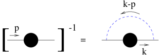
Figure 1: Schwinger-Dyson equation for the fermion self-energy function $\Sigma(p)$ in the rainbow approximation. The dashed line represents the technigluon propagator and the solid line technifermion propagator.

In order to proceed further, however, we need to understand how large $\gamma_{m}$ can be and how walking affects the technicolor chiral symmetry breaking dynamics. These questions cannot be addressed in perturbation theory. Instead, what is conventionally done is to use a nonperturbative approximation for $\gamma_{m}$ and chiral-symmetry breaking dynamics based on the “rainbow” approximation[31, 32] to the Schwinger-Dyson equation shown in Figure 1. Here we write the full, nonperturbative, fermion propagator in momentum space as

$$iS^{-1}(p)=Z(p)(\hbox to0.0pt{\hbox to5.03125pt{\hfil/\hfil}\hss}p-\Sigma(p))~{}.$$ (25)

The linearized form of the gap equation in Landau gauge (in which $Z(p)\equiv 1$ in the rainbow approximation) is

$$\Sigma(p)=3C_{2}(R)\,\int{d^{4}k\over{(2\pi)^{4}}}\,{\alpha_{TC}((k-p)^{2})\over{(k-p)^{2}}}\,{\Sigma(k)\over{k^{2}}}~{}.$$ (26)

Being separable, this integral equation can be converted to a differential equation which has the approximate (WKB) solutions[33, 34]

$$\Sigma(p)\propto p^{-\gamma_{m}(\mu)}\,,\,\,p^{\gamma_{m}(\mu)-2}\,.$$ (27)

Here $\alpha(\mu)$ is assumed to run slowly, as will be the case in walking technicolor, and the anomalous dimension of the fermion mass operator is

$$\gamma_{m}(\mu)=1-\sqrt{1-{\alpha_{TC}(\mu)\over\alpha_{C}}}\,;\ \ \ \ \ \alpha_{C}\equiv{\pi\over 3C_{2}(R)}\,.$$ (28)

One can give a physical interpretation of these two solutions[35, 36] in eq. 27. Using the operator product expansion, we find

$$\lim_{p\to\infty}\Sigma(p)\ \ \propto\ \ \lower 15.0pt\hbox{\epsfbox{figures/ope.eps}}~{}.$$ (29)

Thus the first solution corresponds to a “hard mass” or explicit chiral symmetry breaking, while the second solution corresponds to a “soft mass” or spontaneous chiral symmetry breaking. If we let $m_{0}$ be the explicit mass of a fermion, dynamical symmetry breaking occurs only if

$$\lim_{m_{0}\to 0}\Sigma(p)\neq 0\,.$$ (30)

A careful analysis of the gap equation, or equivalently the appropriate effective potential,[37] implies that this happens only if $\alpha_{TC}$ reaches the critical value of chiral symmetry breaking, $\alpha_{C}$ defined in eq. (28). Furthermore, the chiral symmetry breaking scale $\Lambda_{TC}$ is defined by the scale at which

$$\alpha_{TC}(\Lambda_{TC})=\alpha_{C}$$ (31)

and, hence, at least in the rainbow approximation, at which

$$\gamma_{m}(\Lambda_{TC})=1.$$ (32)

In the rainbow approximation, then, chiral symmetry breaking occurs when the “hard” and “soft” masses scale the same way. It is believed that even beyond the rainbow approximation one will find $\gamma_{m}=1$ at the critical coupling.[38, 39, 40]

3.2 Implications of Walking: Fermion and PGB Masses

If $\beta(\alpha_{TC})\simeq 0$ all the way from $\Lambda_{TC}$ to $M_{ETC}$, then $\gamma_{m}(\mu)\cong 1$ in this range. In this case, eq. (9) becomes

$$m_{q,l}={g^{2}_{ETC}\over{M^{2}_{ETC}}}\times\left(\langle\overline{T}T\rangle_{ETC}\cong\langle\overline{T}T\rangle_{TC}\,{M_{ETC}\over{\Lambda_{TC}}}\right)~{}.$$ (33)

We have previously estimated that flavor-changing neutral current requirements imply that the ETC scale associated with the second generation must be greater than of order 100 to 1000 TeV. In the case of walking technicolor the enhancement of the technifermion condensate implies that

$$m_{q,l}\simeq{{50\,-\,500{\rm\,MeV}}\over N^{3/2}_{D}\theta^{2}_{sd}}~{},$$ (34)

arguably enough to accommodate the strange and charm quarks.

In addition to modifying our estimate of the relationship between the ETC scale and ordinary fermion masses, walking also influences the size of pseudo-Goldstone boson masses. In the case of walking, Dashen’s formula for the size of pseudo-Goldstone boson masses in the presence of chiral symmetry breaking from ETC interactions, eq. (21), reads:

$$F^{2}_{TC}M^{2}_{\pi_{T}} \propto {g^{2}_{ETC}\over M^{2}_{ETC}}\langle\left(\overline{T}T\right)^{2}\rangle)_{ETC}$$ (35)

$$\approx {g^{2}_{ETC}\over M^{2}_{ETC}}\left(\langle\overline{T}T\rangle_{ETC}\right)^{2}$$

$$\simeq {g^{2}_{ETC}\over M^{2}_{ETC}}{M^{2}_{ETC}\over\Lambda^{2}_{TC}}\left(\langle\overline{T}T\rangle_{TC}\right)^{2}\,.$$

Consistent with the rainbow approximation, we have used the vacuum-insertion to estimate the strong matrix element. Therefore we find

$$M_{\pi_{T}} \simeq g_{ETC}\left({4\pi F^{2}_{TC}\over\Lambda_{TC}}\right)$$ (36)

$$\simeq g_{ETC}\left({750{\rm\,GeV}\over N_{D}}\right)\left({1{\rm\,TeV}\over\Lambda_{TC}}\right)~{},$$

i.e. walking also enhances the size of pseudo-Goldstone boson masses! As shown in the discussion of eq. 22, such an enhancement is welcome.

While this is very encouraging, two caveats should be kept in mind. First, the estimates given are for the limit of “extreme walking”, i.e. assuming that the technicolor coupling walks all the way from the technicolor scale $\Lambda_{TC}$ to the relevant ETC scale $M_{ETC}$. To produce a more complete analysis, ETC-exchange must be incorporated into the gap-equation technology in order to estimate ordinary fermion masses. Studies of this sort are encouraging; it appears possible to accommodate the first and second generation masses without necessarily having dangerously large flavor-changing neutral currents.[25, 26, 27, 28, 29, 30] The second issue, however, is what about the third generation quarks, the top and bottom? Because of the large top-quark mass, further refinements[1] or modifications will be necessary to produce a viable theory of dynamical electroweak symmetry breaking. This issue remains the outstanding obstacle in ETC or any theory of flavor. Various models, including top condensate, top seesaw, and top-color assisted technicolor have been proposed; many are discussed by Elizabeth Simmons in her lectures in this volume.

Lectures 2 & 3: Compositeness

4 What is Compositeness?

The relevant phenomenological question is: can any of the observed gauge bosons, the quarks and leptons, or the Higgs boson (if it exists) be composite particles? As we shall quantify in this lecture, the fact that the standard model works well implies that a successful theory must be one in which

• the short distance degrees of freedom are not the same as the long distance degrees of freedom, and

• the masses of the composite states are much less than the intrinsic scale of the dynamics $\Lambda$.

In order to obtain light bound states, the binding energy must be comparable to the intrinsic scale $\Lambda$ and, therefore, the bound states must be relativistic and the theory must be strongly-coupled. We will be discussing field theories in which these conditions are satisfied.

As the masses of the composite states are less than the intrinsic scale ($\Lambda$) of the underlying dynamics, there must be a consistent effective field theory valid for energies $E<\Lambda$ describing dynamics in that energy range. In general, we will not be able to completely solve the strongly-interacting underlying dynamics to give a complete description of the low-energy properties of the bound states. However, we may estimate the types and sizes of interactions[9, 11, 49, 50] based on the following principles:

• That which is not forbidden is required: the effective lagrangian will include all interactions consistent with space-time, global, and gauge symmetries (and, in the case of supersymmetric theories, considerations of analyticity).

• No small dimensionless numbers: the interaction coefficients must be consistent with dimensional analysis.

When $\Lambda\to\infty$, i.e. if there is a large hierarchy of scales, the effective theory must reduce to a renormalizable theory up to corrections suppressed by powers of $\Lambda$. From this point of view, the fact that current experimental results are consistent with a renormalizable theory (the standard one-doublet higgs model) only implies that the scale $\Lambda$ must be larger (perhaps substantially larger) than energy scales we have experimentally probed.

4.1 Dimensional Analysis

Dimensional analysis is the key we will use to extract bounds on the scale of compositeness $\Lambda$ from the results of experiments. Using dimensional analysis, we will estimate sizes of interactions involving composite scalars ($\phi$), fermions ($\psi$), and vector bosons ($V^{\mu}$). Since the effective theory should have no small dimensionless numbers, the sizes of these interactions are determined by two parameters:

• $\Lambda$, the scale of the underlying strong dynamics, and

• $g$, the size of typical coupling constants.

As we now show, the natural size of $g$ is $4\pi$. Let us start with[51] the Wilsonian effective action at scale $\Lambda$:

$$S_{\Lambda}={{{\Lambda^{4}}\over g^{2}}}\int d^{4}x\,{\cal L}\left({{g}\phi\over{\Lambda}},{{g}\psi\over{\Lambda^{3/2}}},{{g}V\over{\Lambda}},{\partial\over{\Lambda}}\right)$$ (37)

Here the parameters $\Lambda$ and $g$ are introduced to get the dimensions correct and to account for an extra coupling for each field in an interaction, while the $\Lambda^{4}/g^{2}$ is present to correctly normalize the kinetic energy, e.g.:

$$\partial^{\mu}\phi^{\dagger}\partial_{\mu}\phi={\Lambda^{4}}{{1\over g^{2}}}\left({\partial^{\mu}\over{\Lambda}}\right)\left({{g}\phi^{\dagger}\over{\Lambda}}\right)\left({\partial_{\mu}\over{\Lambda}}\right)\left({{g}\phi\over{\Lambda}}\right)~{}.$$ (38)

Consider[9] a process which receives contributions from one operator at tree-level, and another at $L$-loop order. Any powers of $\Lambda$ must be the same for both contributions. The $1/g^{2}$ pre-factor in $S_{\Lambda}$ “counts” the number of loops and therefore the ratio of the $L$-loop and tree-level contributions is of order

$$\left({g^{2}\over 16\pi^{2}}\right)^{L}$$ (39)

where we have included one $1/16\pi^{2}$ for each loop from 4-D phase space. Neither of the two extreme possibilities for $g$ is self-consistent:

• $g\ll 4\pi$: in this case, the theory would be weakly coupled, in contradiction with our general expectation that theories with composite particles are strongly coupled;

• If $g\gg 4\pi$: here our prescription for the sizes of various couplings would not be stable under a small change in the cutoff scale $\Lambda$.

Hence, we expect ${g={\cal O}(4\pi)}$ is the natural size for couplings in our effective theory.

In the Wilsonian effective theory, one computes with a momentum-space cutoff of order $\Lambda$. All operators consistent with symmetry requirements then contribute at the same order in $\Lambda^{2}$ to each process, making it impractical for use in actual calculations. Instead, we will use a dimensionless regulator and organize computation in powers of $\Lambda^{-1}$. Matching our estimates from such a calculation with those from the Wilsonian approach implies that the rules of dimensional analysis give us the sizes of interaction coefficients defined using a dimensionless regulator renormalized at a scale of order $\Lambda$.

In constructing the effective theory, we must impose all space-time, global, and gauge symmetries by hand. We may also incorporate any external, weakly-coupled fields (e.g. the photon $A^{\mu}$), by including an appropriate suppression factor (e.g. one factor of $e/g$ for every $A^{\mu}$).

4.2 Example: The QCD Chiral Lagrangian

As an example of the use of dimensional analysis in an effective lagrangian, consider the chiral lagrangian in QCD.[52, 53, 10] The approximate $SU(2)_{L}\times SU(2)_{R}$ chiral symmetry of the QCD lagrangian for light quarks is spontaneously broken to isospin, $SU(2)_{V}$, producing three (approximate) Goldstone Bosons $\pi^{a}$ which we identify with the ordinary pions. In terms of the matrix $\tilde{\pi}=\pi^{a}\sigma^{a}/2$, where the $\sigma^{a}$ are the Pauli matrices, we define

$$\Sigma=\exp\left({{2}i{g}\tilde{\pi}\over{\Lambda}}\right)~{},$$ (40)

which transforms as

$$\Sigma\to{L}\Sigma{R^{\dagger}}\ \ \ \ {L},{R}\in SU(2)_{{L},{R}}~{}.$$ (41)

If we write the lagrangian for $\Sigma$ in an expansion in powers of momentum, the lowest order term invariant under the symmetry of eq. 41 is

$$\hskip-20.0pt{1\over 4}{{\Lambda^{4}}\over{g^{2}}}{\rm Tr}\left[\left({\partial^{\mu}\over{\Lambda}}\right)\Sigma\left({\partial_{\mu}\over{\Lambda}}\right)\Sigma^{\dagger}\right]={f^{2}_{\pi}\over 4}{\rm Tr}\left(\partial^{\mu}\Sigma\partial_{\mu}\Sigma^{\dagger}\right)~{},$$ (42)

where we have identified ${\Lambda}/{g}\equiv f_{\pi}\approx 93$ MeV (from the chiral current) and canonically normalized the kinetic energy of the pion fields. It is customary to denote the dimensional scale $gf_{\pi}$ by $\Lambda_{\chi SB}\simeq 1\,{\rm GeV}$. Higher order chirally invariant terms are possible and applying the dimensional rules we find, for example, a term with four powers of momentum

$${f^{2}_{\pi}\over\Lambda^{2}_{\chi SB}}{\rm Tr}\left(\partial^{\mu}\Sigma\partial_{\mu}\Sigma^{\dagger}\right)^{2}~{}.$$ (43)

From this we conclude that chiral perturbation theory ($\chi$PT) an expansion in $p^{2}/\Lambda^{2}_{\chi SB}$.[9, 11]

In reality, chiral symmetry is not exact, as the bare quark mass terms violate the symmetry:

$${\cal L}_{QCD}=\bar{\psi}i\hbox to0.0pt{\hbox to8.55695pt{\hfil/\hfil}\hss}D\psi-\bar{\psi}_{L}M\psi_{R}-\bar{\psi}_{R}M^{\dagger}\psi_{L}~{}.$$ (44)

We can incorporate $M$ as an “external field” in the chiral lagrangian.[12] Consider first the symmetry properties of the quark mass term: ${\cal L}_{QCD}$ is “invariant” under a chiral transformation combined with the redefinition

$$M\to{L}M{R^{\dagger}}\ \ \ \ {L},{R}\in SU(2)_{{L},{R}}~{},$$ (45)

therefore terms incorporating $M$ must also have this property (this is, essentially, an implementation of a generalized Wigner-Eckart theorem). The power-counting for $M$ can be established by considering the “natural size” of the fermion mass

$${{\Lambda^{4}}\over{g^{2}}}\left({{g}\bar{\psi}\over{\Lambda^{3/2}}}\right)\left({{g}\psi\over{\Lambda^{3/2}}}\right)\equiv\Lambda_{\chi SB}\,\bar{\psi}\psi~{},$$ (46)

in the absence of chiral symmetry. Therefore, the small parameter $M/\Lambda_{\chi SB}$ is a measure of explicit chiral symmetry breaking and the leading term in $M$ has the form

$${{\Lambda^{4}}\over{g^{2}}}\left[{\rm Tr}\left({M\over{\Lambda}}\Sigma^{\dagger}\right)+\,h.c.\right]~{}.$$ (47)

This leads to the usual result $m^{2}_{\pi}\simeq\Lambda_{\chi SB}(m_{u}+m_{d})$.

5 The Phenomenology of Compositeness

Using the rules of dimensional analysis, we can investigate the phenomenology of the compositeness of the observed fermions and gauge bosons. To the extent that they appear fundamental, we establish lower bounds on their scale of compositeness.

5.1 Fermions

We begin by considering the quarks and leptons. Compositeness can be expected to produce several phenomenological effects:

1. Form Factors: If ordinary fermions are composite particles, we expect their gauge interactions to have nontrivial form factors. These form factors can be thought of, in analogy with “vector meson dominance” for the pion form-factor in QCD, as arising from processes such as:

        $$\Rightarrow$$      (48)

   yielding changes in four-fermion cross sections of the form

   $$\hat{\sigma}(f\bar{f}\to f^{\prime}\bar{f^{\prime}})\simeq\hat{\sigma}_{sm}\left[1+{\cal O}\left({{{\hat{s}\over\Lambda^{2}}}}\right)\right]~{},$$ (49)

   where $\hat{s}$ is the partonic center-of-mass energy squared of the process.

2. Contact Interactions[54]: If ordinary fermions are composite, they can also directly exchange heavy resonances arising from the interactions responsible for binding the fermions:

   $$\raise 2.0pt\hbox{\includegraphics[width=99.58464pt]{figures/fourfresonance.eps}}\hskip 14.22636pt\raise 20.0pt\hbox{$\Rightarrow$}\hskip 14.22636pt\raise 0.0pt\hbox{\includegraphics[width=49.79231pt]{figures/fourf.eps}}~{}.$$ (50)

   The effect of these interactions on four fermion cross sections

   $$\hat{\sigma}(f\bar{f}\to f^{\prime}\bar{f^{\prime}})\simeq\hat{\sigma}_{sm}\left[1+{\cal O}\left({{g^{2}\,\hat{s}\over 4\pi\alpha_{sm}\,\Lambda^{2}}}\right)\right]~{},$$ (51)

   is expected to be much larger,[54] due to the factor of $g^{2}/4\pi\alpha_{sm}$.

By searching for deviations in four-fermion processes from the predictions of the standard model, we can place bounds on possible contact interactions. In principle, any interactions of the form

$${\cal L}_{FF}={g^{2}\over 2!\,\Lambda^{2}}\,\eta_{LL}(\bar{\psi}_{L}\gamma^{\mu}\psi_{L})(\bar{\psi}_{L}\gamma_{\mu}\psi_{L})+({RR,\,LR})$$ (52)

consistent with chiral symmetry, gauge symmetries, and flavor symmetries may be present. The convention followed in the typical analyses is $\alpha=g^{2}/4\pi=1$. Note that this is lower than would be expected from dimensional analysis and tends to understate the limits on $\Lambda$. In addition, the analyses generally set only one coefficient (e.g. $\eta_{LL}$ or $\eta_{LR}$) to be non-zero at a time, and give it a value of $\pm 1$, which effectively “normalizes” $\Lambda$. Current lower bounds on the scale $\Lambda$ are shown in table 2, and are typically several TeV.[2]

$\Lambda^{+}_{LL}(eeee)>\,3.1\,{\rm TeV}$	OPAL
$\Lambda^{-}_{LL}(eeee)>\,3.8\,{\rm TeV}$
$\Lambda^{+}_{LL}(ee\mu\mu)>\,4.5\,{\rm TeV}$	OPAL
$\Lambda^{-}_{LL}(ee\mu\mu)>\,4.3\,{\rm TeV}$
$\Lambda^{+}_{LL}(ee\tau\tau)>\,3.8\,{\rm TeV}$	OPAL
$\Lambda^{-}_{LL}(eeee)>\,4.0\,{\rm TeV}$
$\Lambda^{+}_{LL}(\ell\ell\ell\ell)>\,5.2\,{\rm TeV}$	OPAL
$\Lambda^{-}_{LL}(\ell\ell\ell\ell)>\,5.3\,{\rm TeV}$
$\Lambda^{+}_{LL}(eeqq)>\,4.4\,{\rm TeV}$	OPAL
$\Lambda^{-}_{LL}(eeqq)>\,2.8\,{\rm TeV}$
$\Lambda^{+}_{LL}(\nu\nu qq)>\,5.0\,{\rm TeV}$	NUTEV
$\Lambda^{-}_{LL}(\nu\nu qq)>\,5.4\,{\rm TeV}$
$\Lambda^{\pm}_{LL}(qqqq)>\,1.9\,{\rm TeV}$	DØ

Table 2: Current limits on the scale $\Lambda$ for compositeness derived from various four-fermion scattering experiments.[2]

5.2 Gauge Bosons

Next we consider the possibility that the ordinary gauge bosons are composite objects. At first sight this seems unreasonable, since these particles are associated with a local gauge symmetry. However, as shown by Weinberg,[55] for consistency any massless vector particle must couple to a conserved current – i.e. the existence of a “gauge symmetry” is automatic for any massless spin-1 particle.

Dimensional analysis allows us to estimate the size of the resulting couplings. The natural size of the coupling constant is ${\cal O}(4\pi)$, as can be seen by considering a generic three-point coupling:

$${{\Lambda^{4}}\over{g^{2}}}\,\left({\partial\over{\Lambda}}\right)\left({{g}V\over{\Lambda}}\right)^{3}\equiv g(\partial V)VV~{}.$$ (53)

However, the standard model gauge interactions are asymptotically free and their couplings at high energies ($\simeq 1$ TeV) are small. For this reason, it is likely that the $\gamma$, $g$, $W^{\pm}_{T}$, $Z_{T}$ are fundamental.

The situation is quite different for the longitudinally polarized weak gauge bosons, the $W^{\pm}_{L}$ and $Z_{L}$. These particles are “eaten” Goldstone bosons, have effective couplings to each other proportional to momentum and, as discussed in the previous lecture, they are not fundamental in theories of dynamical electroweak symmetry breaking. The effective lagrangian for a theory of massive electroweak bosons with composite longitudinal modes includes the fundamental $W_{T}$ and $B_{T}$ gauge bosons of $SU(2)_{W}\times U(1)_{Y}$ symmetry. In addition, just as in the chiral lagrangian in QCD, we may describe the Goldstone bosons of electroweak symmetry breaking by a matrix $\Sigma$ which transforms to $L\Sigma R^{\dagger}$ under a global $SU(2)_{L}\times SU(2)_{R}$ which is broken to $SU(2)_{V}$. As discussed previously, the residual “custodial” $SU(2)_{V}$ symmetry ensures[5, 6] that the weak interaction $\rho$ parameter (eq. 7) is equal to 1.

The low-energy of effects of dynamical electroweak symmetry breaking include anomalous weak gauge-boson couplings described by the effective lagrangian described above. These corrections can be thought of as due to the exchange of the lightest resonances likely to be present in such theories, “technirho” vector mesons ($\rho_{TC}$) analogous to the $\rho$ in QCD. Such corrections modify the 3-pt functions:

(54)

yielding the couplings

$$-\ i\,{g_{SU(2)}}{{\it l}_{9L}\over 16\pi^{2}}\,{\rm Tr}{{{\rm\bf W}^{\mu\nu}}D_{\mu}\Sigma D_{\nu}\Sigma^{\dagger}}~{},$$ (55)

and

$$-\ i\,{g^{\prime}_{U(1)}}{{\it l}_{9R}\over 16\pi^{2}}\,{\rm Tr}{{B^{\mu\nu}}D_{\mu}\Sigma^{\dagger}D_{\nu}\Sigma}~{}.$$ (56)

In these expressions we have taken ${g}\simeq 4\pi$, so the l’s are normalized to be O(1).

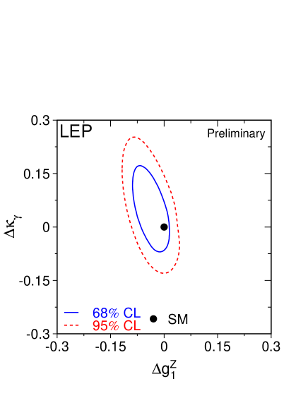
Figure 2: Current limits[56] on the anomalous weak gauge-boson coupling parameters $\kappa_{\gamma}$ and $g^{Z}_{1}$.

The conventional[57] description of anomalous weak gauge-boson couplings was given by Hagiwara, et. al.:

$${i\over e\cot\theta} {\cal L}_{WWZ}=g_{1}(W^{\dagger}_{\mu\nu}W^{\mu}Z^{\nu}-W^{\dagger}_{\mu}Z_{\nu}W^{\mu\nu})$$

$$+\kappa_{Z}W^{\dagger}_{\mu}W_{\nu}Z^{\mu\nu}+{\lambda_{Z}\over M_{W}^{2}}W^{\dagger}_{\lambda\mu}W^{\mu}_{\nu}Z^{\nu\lambda}~{},$$

and

$${i\over e} {\cal L_{WW\gamma}}=(W^{\dagger}_{\mu\nu}W^{\mu}A^{\nu}-W_{\mu}^{\dagger}A_{\nu}W^{\mu\nu})$$

$$+\kappa_{\gamma}W^{\dagger}_{\mu}W_{\nu}F^{\mu\nu}+{\lambda_{\gamma}\over M_{W}^{2}}W^{\dagger}_{\lambda\mu}W^{\mu}_{\nu}F^{\nu\lambda}~{}.$$

Comparing with the interactions above (in unitary gauge, $\Sigma\equiv{\cal I}$), we find:

$$\left.\begin{array}[]{c}g_{1}-1\\ \kappa_{Z}-1\\ \kappa_{\gamma}-1\end{array}\right\}\ \approx\ {\alpha_{*}l_{i}\over 4\pi\sin^{2}\theta}={\cal O}(10^{-2}-10^{-3})~{}.$$ (59)

The couplings $\lambda_{Z,\gamma}$ arise from higher order interactions, and are estimated to be ${\cal O}(10^{-4}-10^{-5})$. Current limits from LEP are shown in fig. 2. These data show agreement with the standard model, but do not set useful limits.

For your consideration…

1. If quarks and leptons are composite, one expects there are excited states with the same quantum numbers (typically denoted $\ell^{*}$ and $q^{*}$). The PDG[2] lists bounds on excited states of quarks and leptons of ${\cal O}(100\,{\rm GeV})$.

   • Based on dimensional analysis, what bound does this place on the scale of compositeness $\Lambda$?

2. BNL experiment E-821 will measure the anomalous magnetic moment of the muon to 0.35 ppm.

   • Show using dimensional analysis that this is measurement should be sensitive to one-loop weak corrections.

   • If the experiment agrees with the SM, what bound will this measurement place on the scale of muon compositeness?

6 Composite Higgs Bosons

Up to now, our discussion of compositeness has consisted of the construction of consistent effective low-energy theories and an analysis of current experimental lower bounds on the scale of compositeness of the observed particles. In order to proceed, we need to understand the characteristics of plausible fundamental high-energy theories which give rise to light (possibly massless) composite states. In this section we consider models which give rise to composite scalars, and in particular a Higgs Boson. In subsequent sections, we will describe models giving rise to composite fermions and gauge bosons.

6.1 Top-Condensate Models

The fact that the top quark, with $m_{t}\simeq 2M_{W},\,2M_{Z}$, is much heavier than other fermions implies that the top is more strongly coupled to the EWSB sector. This has led to the construction of models in which all[59, 60, 61, 62, 63, 64, 65, 66, 67] or some[68] of electroweak symmetry breaking is due to top condensation, $\langle\bar{t}t\rangle\neq 0$.

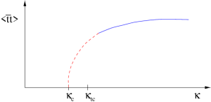
Figure 3: Top-quark condensate produced in NJL approximation to topcolor dynamics as a function of the coupling $\kappa$. Condensate forms only for $\kappa>\kappa_{c}$ and, at least in this approximation, the condensate turns on continuously -- i.e. the quantum chiral phase transition is second order.

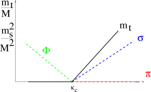
Figure 4: Spectrum of low-energy states in any model with a second order quantum chiral phase transition. The spectrum must change smoothly at the critical coupling; there must be massless fermions below the critical coupling and massless Goldstone bosons above the critical coupling.

The simplest model involves a spontaneously broken but strong topcolor[64] gauge interaction

$${SU(3)_{tc}}\times{SU(3)}\stackrel{{\scriptstyle M}}{{\to}}SU(3)_{QCD}$$ (60)

which couples preferentially to the third generation of quarks. At energies small compared to the mass ($M$) of the topgluon, such an interaction gives rise to a local four-fermion operator

$${\cal L}\supset-{4\pi\kappa\over 2!\,M^{2}}\left(\overline{Q}\gamma_{\mu}{\lambda^{a}\over 2}Q\right)^{2}$$ (61)

where $\kappa\propto g^{2}_{tc}(M)$, the $\lambda^{a}$ are the Gell-mann matrices, and the fields $Q$ are the doublets (left- and right-handed, for the model as described so far) third generation weak doublet fields.

This model may be solved[69] in the ‘‘NJL approximation’’ in the large-$N_{c}$ limit. The behavior of the chiral symmetry breaking condensate is shown in fig. 4, with:

$${\langle\bar{t}t\rangle\over M^{3}}\propto\sqrt{\Delta\kappa\over\kappa_{c}}\equiv\sqrt{{\kappa-\kappa_{c}}\over\kappa_{c}}~{}.$$ (62)

The condensate changes smoothly from zero as $\kappa$ exceeds the critical value $\kappa_{c}$; this behavior represents a second order chiral phase transition. Clearly, if $M\gg 1{\rm\,TeV}$ and the dynamics of topcolor occurs at scales much higher than 1 TeV, the value of $\kappa$ must be tuned close to $\kappa_{c}$.

Assuming the transition is second order, as motivated by the NJL calculation, it is easy to understand the form of the effective low-energy field theory when $\kappa$ is just slightly greater than $\kappa_{c}$. As shown in fig. 4, the light degrees of freedom include the top-quark, the Goldstone bosons eaten by the $W$ and $Z$, as well as a singlet scalar particle (the $\sigma$). In order for this theory to have a smooth limit as $\kappa\to\kappa^{+}_{c}$, the $\sigma$ and the Goldstone bosons must arrange themselves to form a light composite Higgs boson!

In fact, for the theory as described, we have not distinguished the top from the bottom quark. The theory includes two light Higgs doublets in a $2\times 2$ matrix field $\Phi$ as required in an $SU(2)_{L}\times SU(2)_{R}$ linear sigma model. Using our rules of dimensional analysis, the most general effective lagrangian describing the light fields is:

$${\cal L}_{eff}={\rm Tr}\left(\partial^{\mu}\Phi^{\dagger}\partial_{\mu}\Phi\right)+\bar{\psi}\hbox to0.0pt{\hbox to5.30904pt{\hfil/\hfil}\hss}\partial\psi+y\,\bar{\psi}\Phi\psi+{\cal O}\left({\partial^{2}\over M^{2}}\right)~{}.$$ (63)

Note that, the absence of a Higgs mass term ($m^{2}{\rm Tr}(\Phi^{\dagger}\Phi)$) is due entirely to the dynamical assumption that we are (very) close to the transition ($|m^{2}|\ll M^{2}$). Dimensional analysis implies that $y={\cal O}(4\pi)$ and a heavy top quark arises naturally.

The Higgs (at large $N_{c}$ in the NJL approximation) can be found directly as pole in the sum of bubble sum diagrams[63]

$$\epsfbox{figures/bubblesum.eps}~{}.$$ (64)

The eaten Goldstone bosons arise in the corresponding diagrams for the $W/Z$ self-energies:

$$\epsfbox{figures/Wmass.eps}~{},$$ (65)

and implies a Higgs vacuum expectation value

$$f_{t}^{2}={N_{c}\over 4\pi}\int^{\Lambda}{k^{2}dk^{2}m_{t}^{4}\over(k^{2}+m_{t}^{2})^{2}}~{}.$$ (66)

A number of phenomenological issues must be addressed prior to constructing a realistic model based on topcolor. First, additional ‘‘tilting’’ interactions must be introduced to ensure that the bottom quark is not heavy, i.e. $\langle\bar{b}b\rangle\approx 0$. Second, some account must be given of the observed mixing between the third generation and the first two. Finally, top quark condensation alone produces only a Higgs vacuum expectation value of $f_{t}\approx 60$ GeV, which is too small to account for electroweak symmetry breaking.[63]

The simplest model of a single composite Higgs boson based on top-condensation is the top seesaw model.[66, 67] In this model, electroweak symmetry breaking is due to the condensate of the left-handed top quark $t_{L}$ with a new right-handed weak singlet quark $\chi_{R}$. While $\langle t_{L}\chi_{R}\rangle$ is responsible for all of electroweak symmetry breaking, mixing of the top with left- and right-handed singlet quarks yields a seesaw mass matrix

$${\lower 55.0pt\hbox{\includegraphics*[width=142.26378pt]{figures/tseesaw.eps}}}\hskip 10.0pt{\pmatrix{\overline{t_{L}}&\overline{\chi_{L}}\cr}\,\pmatrix{0&m_{t\chi}\cr\mu_{\chi t}&\mu_{\chi\chi}\cr}\pmatrix{t_{R}\cr\chi_{R}\cr}}$$ (67)

which gives rise to the observed mass-eigenstate top-quark.

6.2 The Triviality of the Standard Higgs Model

A composite Higgs is also motivated by the fact that the standard one-doublet Higgs model does not strictly exist as a continuum field theory. This result is most easily illustrated in terms of the Wilson renormalization group.[71, 72, 73] Any quantum field theory is defined using a regularization procedure which ameliorates the bad short-distance behavior of the theory. Following Wilson, we define the scalar sector of the standard model

$${\cal L}_{\Lambda}= D^{\mu}\phi^{\dagger}D_{\mu}\phi+m^{2}(\Lambda)\phi^{\dagger}\phi+{\lambda(\Lambda)\over 4}(\phi^{\dagger}\phi)^{2}$$

$$+{\eta(\Lambda)\over 36\Lambda^{2}}(\phi^{\dagger}\phi)^{3}+\ldots$$

in terms of a fixed UV-cutoff $\Lambda$. Here we have allowed for the possibility of terms of (engineering) dimension greater than four. While there are an infinite number of such terms, one representative term of this sort, $(\phi^{\dagger}\phi)^{3}$, has been included explicitly for the purposes of illustration. Note that the coefficient of the higher dimension terms includes the appropriate number of powers of $\Lambda$, the intrinsic scale at which the theory is defined.

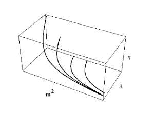
Figure 5: Graphical representation of Wilson RG flow of $(m^{2}(\Lambda),\lambda(\Lambda),\eta(\Lambda))$. As we scale to low energies, $m^{2}\to\infty$, $\lambda\to 0$, and $\eta\to 0$.

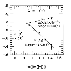
Figure 6: Results of a nonperturbative lattice monte carlo study [74] of the scalar sector of the standard model with bare coupling $\lambda=10$. The approximate slope of -1 for the renormalized coupling, $\lambda_{R}$, shows agreement with the naive one-loop perturbative result.

Wilson observed that, for the purposes of describing experiments at some fixed low-energy scale $E\ll\Lambda$, it is possible to trade a high-energy cutoff $\Lambda$ for one that is slightly lower, $\Lambda^{\prime}$, so long as $E\ll\Lambda^{\prime}<\Lambda$. In order to keep low-energy measurements fixed, it will in general be necessary to redefine the values of the coupling constants that appear in the Lagrangian. Formally, this process is referred to as ‘‘integrating out’’ the (off-shell) intermediate states with $\Lambda^{\prime}<k<\Lambda$. Keeping the low-energy properties fixed we find

$${\cal L}_{\Lambda} \Rightarrow {\cal L}_{\Lambda^{\prime}}$$

$$m^{2}(\Lambda) \rightarrow m^{2}(\Lambda^{\prime})$$ (69)

$$\lambda(\Lambda) \rightarrow \lambda(\Lambda^{\prime})$$

$$\eta(\Lambda) \rightarrow \eta(\Lambda^{\prime})~{}.$$

Wilson’s insight was to see that many properties of the theory can be summarized in terms of the evolution of these (generalized) couplings as we move to lower energies. Truncating the infinite-dimensional coupling constant space to the three couplings shown above, the behavior of the scalar sector of the standard model is illustrated in Figure 6. This figure illustrates a number of important features of scalar field theory. As we flow to the infrared, i.e. lower the effective cutoff, we find:

• $\eta\to 0$ --- this is the modern interpretation of renormalizability. If $m_{H}\ll\Lambda$, the theory is drawn to the two-dimensional $(m_{H},\lambda)$ subspace. Any theory in which $m_{H}\ll\Lambda$ is therefore close to a renormalizable theory with corrections suppressed by powers of $\Lambda$.

• $m^{2}\to\infty$ --- This is the naturalness or hierarchy problem. To maintain $m_{H}\simeq{\cal O}(v)$ we must adjust  the value of $m_{H}$ in the underlying theory to of order

  $${\Delta m^{2}(\Lambda)\over m^{2}(\Lambda)}\propto{v^{2}\over\Lambda^{2}}~{}.$$ (70)

• $\lambda\to 0$ --- The coupling $\lambda$ has a positive $\beta$ function and, therefore, as we scale to low energies $\lambda$ tends to 0. If we try to take the ‘‘continuum’’ limit, $\Lambda\to+\infty$, the theory becomes free or trivial.[71, 72, 73]

The triviality of the scalar sector of the standard one-doublet Higgs model implies that this theory is only an effective low-energy theory valid below some cut-off scale $\Lambda$. Given a value of $m^{2}_{H}=2\lambda(m_{H})v^{2}$, there is an upper bound on $\Lambda$. An estimate of this bound can be obtained by integrating the one-loop $\beta$-function, which yields

$$\Lambda\begin{array}[]{c}<\vspace{-0.5em}\\ {\scriptstyle\sim}\end{array}m_{H}\exp\left({4\pi^{2}v^{2}\over 3m^{2}_{H}}\right)~{}.$$ (71)

For a light Higgs, the bound above is at uninterestingly high scales and the effects of the underlying dynamics can be too small to be phenomenologically relevant. For a Higgs mass of order a few hundred GeV, however, effects from the underlying physics can become important. I will refer to these theories generically as ‘‘composite Higgs’’ models.

Finally, while the estimate above is based on a perturbative analysis, nonperturbative investigations of $\lambda\phi^{4}$ theory on the lattice show the same behavior. This is illustrated in Figure 6.

6.3 $T$, $S$, and $U$ in Composite Higgs Models

In an $SU(2)_{W}\times U(1)_{Y}$ invariant scalar theory of a single doublet, all interactions of dimension less than or equal to four also respect a larger ‘‘custodial’’ symmetry [5, 6] which insures the tree-level relation $\rho=M^{2}_{W}/M^{2}_{Z}\cos^{2}\theta_{W}\equiv 1$ is satisfied. The leading custodial-symmetry violating operator is of dimension six [75, 76] and involves four Higgs doublet fields $\phi$. In general, the underlying theory does not respect the larger custodial symmetry, and we expect the interaction

$${\lower 35.0pt\hbox{\epsfbox{figures/fourhiggs.eps}}}\Rightarrow{b{\kappa}^{2}\over 2!\,{\Lambda}^{2}}(\phi^{\dagger}\stackrel{{\scriptstyle\leftrightarrow}}{{D^{\mu}}}\phi)^{2}~{},$$ (72)

to appear in the low-energy effective theory. Here $b$ is an unknown coefficient of ${\cal O}(1)$, and ${\kappa}$ measures size of couplings of the composite Higgs field. In a strongly-interacting theory, $\kappa$ is expected [11, 49] to be of ${\cal O}(4\pi)$.

Deviations in the low-energy theory from the standard model can be summarized in terms of the ‘‘oblique’’ parameters [41, 42, 43, 44, 45] $S$, $T$, and $U$. The operator in eq. 72 will give rise to a deviation ($\Delta\rho=\varepsilon_{1}=\alpha T$)

$${|\Delta T|}={|b|{\kappa}^{2}{v^{2}\over\alpha(M_{Z}){\Lambda}^{2}}}{\begin{array}[]{c}>\vspace{-0.5em}\\ {\scriptstyle\sim}\end{array}}{|b|\kappa^{2}\,v^{2}\over\alpha(M^{2}_{Z})\,m^{2}_{H}}\,\exp\left({-\,{8\pi^{2}v^{2}\over 3m^{2}_{H}}}\right)~{},$$ (73)

where $v\approx 246$ GeV and we have used eq. 71 to obtain the final inequality. The consequences of eqns. (71) and (73) are summarized in Figures 8 and 8. The larger $m_{H}$, the lower $\Lambda$ and the larger the expected value of $\Delta T$. Current limits imply $|T|\stackrel{{\scriptstyle<}}{{\sim}}0.5$, and hence[77] ${\Lambda\stackrel{{\scriptstyle>}}{{\sim}}4\,{\rm TeV}\cdot\kappa}$. (For $\kappa\simeq 4\pi$, $m_{H}\begin{array}[]{c}<\vspace{-0.5em}\\ {\scriptstyle\sim}\end{array}450$ GeV.)

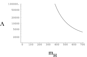
Figure 7: Upper bound on scale $\Lambda$ as per eq. (71).

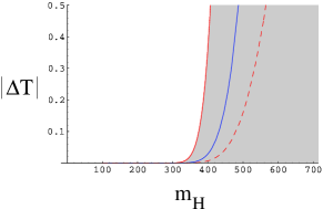
Figure 8: Lower bound on expected size of $|\Delta T|$ as per eq. (73), for $|b|\kappa^{2}=16\pi^{2}$, $4\pi$, and 3.

By contrast, the leading contribution to $S$ arises from

$${\lower 35.0pt\hbox{\epsfbox{figures/shiggs.eps}}}\Rightarrow-\,{a\over 2!\,{\Lambda}^{2}}\left\{[D_{\mu},D_{\nu}]\phi\right\}^{\dagger}[D^{\mu},D^{\nu}]\phi~{}.$$ (74)

This gives rise to ($\varepsilon_{3}={\alpha S/4\sin^{2}\theta_{W}}$)

$$\Delta S={4\pi av^{2}\over{\Lambda}^{2}}~{}.$$ (75)

It is important to note that the size of contributions to $\Delta T$ and $\Delta S$ are very different

$${\Delta S\over\Delta T}={a\over b}\left({4\pi\alpha\over{\kappa}^{2}}\right)={\cal O}\left({10^{-1}\over{\kappa}^{2}}\right)~{}.$$ (76)

Even for ${\kappa}\simeq 1$, $|\Delta S|\ll|\Delta T|$.

Finally, contributions to $U$ ($\varepsilon_{2}=-{\alpha U\over 4\sin^{2}\theta_{W}}$), arise from

$${cg^{2}{\kappa^{2}}\over\Lambda^{4}}(\phi^{\dagger}W^{\mu\nu}\phi)^{2}$$ (77)

and, being suppressed by $\Lambda^{4}$, are typically much smaller than $\Delta T$.

6.4 Limits on a Composite Higgs Boson

From triviality, we see that the Higgs model can only be an effective theory valid below some high-energy scale $\Lambda$. As the Higgs becomes heavier, the scale $\Lambda$ decreases. Hence, the expected size of contributions to $T$ grow, and are larger than the expected contribution to $S$ or $U$. The limits from precision electroweak data in the $(m_{H},\Delta T)$ plane are shown in Figure 9. We see that, for positive $\Delta T$ at 95% CL, the allowed values of the Higgs mass extend to well beyond 800 GeV. On the other hand, not all values can be realized consistent with the bound given in eq. (71). As shown in figure 9, values of the Higgs mass beyond approximately 500 GeV would likely require values of $\Delta T$ much larger than allowed by current measurements.

Figure 9: 68% and 95% CL regions allowed [78] in $(m_{H},|\Delta T|)$ plane by precision electroweak data.[79] Fit allows for $m_{t}$, $\alpha_{s}$, and $\alpha_{em}$ to vary consistent with current limits.[78] Also shown by the dot-dash curve is the contour corresponding to $\Delta\chi^{2}=4$, whose intersection with the line $\Delta T=0$ -- at approximately 190 GeV -- corresponds to the usual 95% CL upper bound quoted on the Higgs boson mass in the standard model. The triviality bound curves are for $|b|\kappa^{2}=4\pi$ and $4\pi^{2}$, corresponding to representative models.[78]

I should emphasize that these estimates are based on dimensional arguments. I am not arguing that it is impossible to construct a composite Higgs model consistent with precision electroweak tests with $m_{H}$ greater than 500 GeV. Rather, barring accidental cancellations in a theory without a custodial symmetry, contributions to $\Delta T$ consistent with eq. 71 are generally to be expected. In particular composite Higgs boson models, the bounds given here have been shown to apply.[78]

These results may also be understood by considering limits in the $(S,T)$ plane for fixed $(m_{H},m_{t})$. In Figure 11, changes from the nominal standard model best fit ($m_{H}=84$ GeV) value of the Higgs mass are displayed as contributions to $\Delta S(m_{H})$ and $\Delta T(m_{H})$. Also shown are the 68% and 95% CL bounds on $\Delta S$ and $\Delta T$ consistent with current data. We see that, for $m_{H}$ greater than ${\cal O}$(200 GeV), a positive contribution to $T$ can bring the model within the allowed region.

At Run II of the Fermilab Tevatron, it may be possible to reduce the uncertainties in the top-quark and W-boson masses to $\Delta m_{t}=2$ GeV and $\Delta M_{W}=30$ MeV.[80] Assuming that the measured values of $m_{t}$ and $M_{W}$ equal their current central values, such a reduction in uncertainties will result the limits in the $(m_{H},\Delta T)$ plane shown in Figure 11. Note that, despite reduced uncertainties, a Higgs mass of up to 500 GeV or so will still be allowed.

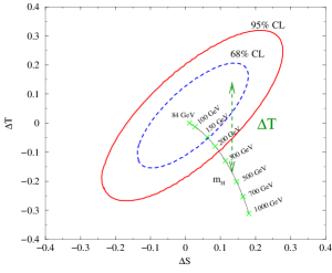
Figure 10: 68% and 95% CL regions allowed in $(\Delta S,\Delta T)$ plane by precision electroweak data.[79] Fit allows for $m_{t}$, $\alpha_{s}$, and $\alpha_{em}$ to vary consistent with current limits.[78] Standard model prediction for varying Higgs boson mass shown as parametric curve, with $m_{H}$ varying from 84 to 1000 GeV.

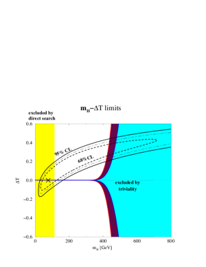
Figure 11: 68% and 95% CL allowed region [78] in $(m_{H},\Delta T)$ plane if Fermilab Tevatron Run II reduces the uncertainty in top-quark and W-boson masses to $\Delta m_{t}=2$ GeV and $\Delta M_{W}=30$ MeV about their current central values.

7 Composite Fermions

7.1 Chiral Symmetry and Anomalies

Consider a chiral transformation of a 4-component Dirac field:

$$\psi\to e^{+i\alpha\gamma_{5}}\psi\hskip 10.0pt\Leftrightarrow\hskip 10.0pt\psi_{L,R}\to e^{\pm i\alpha}\psi_{L,R}~{},$$ (78)

which may also be written

$$\psi_{L}\to e^{+i\alpha}\psi_{L}\hskip 10.0pt\&\hskip 10.0pt{\cal C}\psi_{R}\equiv\psi^{c}_{L}\to e^{+i\alpha}\psi^{c}_{L}~{},$$ (79)

in terms of the charge-conjugate field $\psi^{c}_{L}$. Since fermion mass terms

$$m\bar{\psi}\psi\hskip 10.0pt\Leftrightarrow\hskip 10.0ptm\bar{\psi_{L}}\psi_{R}+{h.c.}$$ (80)

couple the left- and right-handed components of a fermion field, mass terms are not chirally invariant. Therefore, an unbroken global chiral symmetry is a sufficient condition for the existence of massless fermions at low energies. If these massless fermions are composite objects, the fundamental fermions of which they are composed must carry the same symmetries. ’t Hooft realized[81] that there were additional constraints relating the representations of the fundamental and composite fermions: the anomaly matching conditions.

We begin our discussion with a review of anomalies in quantum field theory. Regularization of quantum field theory, necessary to extract finite answers, generally breaks various global symmetries of the model, and one must re-impose these symmetries upon renormalization. However, regularization always breaks chiral symmetries and, surprisingly, we generally cannot re-impose both[82, 83, 84, 85] vector and chiral symmetries in renormalized theory! The result is that a symmetry of the classical theory is broken at quantum level. Hence, the use of the term anomaly.

In perturbation theory, the anomaly manifests itself in the behavior of the triangle diagram

$$\lower 20.0pt\hbox{\includegraphics*[width=85.35826pt]{figures/avv.eps}}~{}.$$ (81)

Imposing vector current conservation, one finds that the divergence of the axial current is nonzero:

$$\langle p,\nu,b;k,\lambda,c|\partial_{\mu}A^{a\mu}|0\rangle={1\over 4\pi^{2}}\,\varepsilon^{\alpha\nu\beta\lambda}\,p_{\alpha}k_{\beta}\,\cdot{\rm Tr}(T^{a}\{T^{b},T^{c}\})~{}.$$ (82)

For simplicity, we will write the theory, and symmetries, in terms of left-handed fermions and currents only. Diagrammatically, one can move the chiral projector $\left({{1-\gamma_{5}}\over 2}\right)$ to a single vertex. We will regularize so that the resulting VVV term not anomalous; the AVV term remains as above.

(Gauge)³ Anomalies

Consider first a vectorial $SU(N_{c})$ gauge theory with $N_{f}$ fermions in the fundamental $N_{c}$ representation. The fermions transform as:

$$\psi_{L}:\,(N_{c},N_{f},1)\hskip 15.0pt\psi^{c}_{L}:\,(\bar{N_{c}},1,\bar{N_{f}})$$ (83)

under the $SU(N_{c})$ gauge and $SU(N_{f})_{L}\times SU(N_{f})_{R}$ global symmetries. For consistency, the $SU(N_{c})$ gauge current must be conserved and the corresponding symmetry cannot be anomalous. For a representation $R$, define:

$${\rm Tr}(T^{a}_{R}\{T^{b}_{R},T^{c}_{R}\})\equiv{1\over 2}\,{\cal A}(R)\,d^{abc}~{},$$ (84)

and hence ${\cal A}(N_{c})\equiv 1$. For the $\bar{N_{c}}$ representation:

$${\rm Tr}(T^{a}_{R}\{T^{b}_{R},T^{c}_{R}\})={\rm Tr}((-T^{a})^{T}\{(-T^{b})^{T},(-T^{c})^{T}\})~{},$$ (85)

and ${\cal A}(\bar{N_{c}})=-1$. Hence the total gauge anomaly

$$N_{f}\cdot{\cal A}(N_{c})+N_{f}\cdot{\cal A}(\bar{N_{c}})\equiv 0~{}.$$ (86)

In general, for any real representation the generators $T^{a}_{R}$ are unitarily equivalent to $(-T^{a})^{T}$ and therefore ${\cal A}(R)\equiv 0$.

One can also construct a chiral gauge theory using a complex, but anomaly-free, representation. Consider the two-index antisymmetric tensor representation, $A^{ij}$, of $SU(N)$. Since $d_{abc}$ is a group-theoretic invariant, to calculate ${\cal A}(R)$ one need only consider a single nonvanishing term on the left hand side of eq. 84. In particular, consider the generator proportional to

$$\left(\begin{array}[]{cccc}-1&&&\\ &-1&&\\ &&\ddots&\\ &&&N-1\end{array}\right)$$ (87)

in the fundamental representation. ${\rm Tr}(T^{3})$ implies

$${\cal A}(N)\propto(N-1)\cdot(-1)^{3}+1\cdot(N-1)^{3}$$ (88)

for the fundamental representation $N$ and

$${\cal A}(A)\propto{(N-1)(N-2)\over 2}\cdot(-2)^{3}+(N-1)\cdot(N-2)^{3}$$ (89)

for the antisymmetric tensor representation $A$. A little algebra shows that ${\cal A}(A)=(N-4)\,{\cal A}(N)$, hence we can construct an anomaly-free chiral gauge theory by including fermions transforming as one antisymmetric tensor and $N-4$ antifundamentals.

For your consideration …

Consider one family of quarks and leptons in the standard $SU(3)_{C}\times SU(2)_{W}\times U(1)_{Y}$ model.

Show that all of the following gauge anomalies cancel:

• $(SU(3)_{C})^{3}$

• $(SU(2)_{W})^{3}$

• $(U(1)_{Y})^{3}$

• $(SU(3)_{C})^{2}\,SU(2)_{W}$

• $(SU(2)_{W})^{2}\,SU(3)_{C}$

• $(SU(3)_{C})^{2}\,U(1)_{Y}$

• $(SU(2)_{W})^{2}\,U(1)_{Y}$

• $(U(1)_{Y})^{2}\,SU(3)_{C}$

• $(U(1)_{Y})^{2}\,SU(2)_{W}$

• $SU(3)_{C}\,SU(2)_{W}\,U(1)_{Y}$

• $\{SU(3)_{C},SU(2)_{W},U(1)_{Y}\}\,(Grav)^{2}$

Which connect quark and lepton charges?

Global/Gauge Anomalies

Global chiral symmetries can be violated by anomalies as well. The classic example is axial quark number, $U(1)_{A}$, in QCD. Including this (approximate) classical global symmetry the $N_{f}$ quarks transform as

$$\psi^{i}_{L}:\,(3,N_{f},1)_{+1}\hskip 20.0pt\psi^{c}_{L}:\,(\bar{3},1,\bar{N_{f}})_{+1}$$ (90)

under $SU(3)\times SU(N_{f})_{L}\times SU(N_{f})_{R}\times U(1)_{A}$. The triangle graph

(91)

yields a result proportional to

$${\rm Tr}(T_{U(1)_{A}}\{T^{b},T^{c}\})=N_{f}\,{\rm Tr}\{T_{3}^{b},T_{3}^{c}\}+N_{f}\,{\rm Tr}\{T_{\bar{3}}^{b},T_{\bar{3}}^{c}\}\neq 0~{}.$$ (92)

Consequently,[86] the $U(1)_{A}$ current is not conserved

$${\partial^{\mu}j^{5}_{\mu}=-\,{g_{QCD}^{2}N_{f}\over 32\pi^{2}}\varepsilon^{\alpha\nu\beta\lambda}F^{a}_{\alpha\nu}F^{a}_{\beta\lambda}}~{},$$ (93)

and there is no ninth Goldstone Boson in QCD!

Surprisingly, there is an anomaly-free global $U(1)$ symmetry in the chiral $SU(N)$ model described above. The $U(1)_{global}SU(N)^{2}$ anomaly is proportional to index

$${\rm Tr}\{T^{a}_{R},T^{b}_{R}\}\equiv k(R)\,\delta^{ab}~{}.$$ (94)

of the $SU(N)$ representation of the fermion, which is a group theoretic invariant. Consider generator proportional to

$$\left(\begin{array}[]{ccc}1&&\\ &-1&\\ &&\ddots\\ \end{array}\right)~{}.$$ (95)

The index of a representation is proportional to ${\rm Tr}(T^{2})$, which gives

$$k(N)\propto 2\cdot(1)^{2}+(N-2)\cdot(0)^{2}$$ (96)

for the fundamental representation, and

$$k(A)\propto 1\cdot(0)^{2}+2\cdot(N-2)\cdot(1)^{2}$$ (97)

for the antisymmetric tensor. Recall that the consistent chiral $SU(N)$ theory has one antisymmetric tensor $A$ and $N-4$ antifundamental representations $\bar{N}$. Comparing to eqs. 96 and 97, we see that there is an anomaly-free global $U(1)$ symmetry under which the antisymmetric tensor has charge $-1$ and $(N-4)$ antifundamentals have charge ${{N-2\over N-4}}$. In the simplest nontrivial case, chiral $SU(5)$, the antisymmetric tensor is ten dimensional and the fermion fields transform as $10_{-1}$ and $\bar{5}_{3}$ under $SU(5)\times U(1)$.

7.2 (Global)³ Anomalies: the ‘t Hooft Conditions

The existence of massless composite fermions implies that there is a low-energy global chiral symmetry group $H$, and this group must be a subgroup of the high-energy global symmetries. ‘t Hooft argued[81] that the (global)³ anomaly factor (${\cal A}_{H}$) must be the same in the low- and high-energy theories. His argument runs as follows: consider a theory with massless composite fermions with a global chiral symmetry group $H$. Suppose you were to weakly gauge the chiral global symmetry group $H$. In order to avoid gauge anomalies, one must also add ‘‘spectator’’ fermions which are weakly, but not strongly interacting, to cancel the anomalies ${\cal A}_{H}$. By definition, these weak gauge interactions don’t affect the dynamics, and the massless composite fermions must still form. In order for the weak gauge group to remain consistent, therefore the low-energy massless composites must cancel anomalies of spectator fermions. Hence,

$${\cal A}_{fundamental}={\cal A}_{composite}~{}.$$ (98)

The condition in eq. 98 is a nontrivial relation between the $H$ representations of the fundamental and composite fermions. It provides a necessary condition which must be satisfied by any putative theory of composite fermions. We will illustrate the anomaly matching conditions with two plausible theories of composite massless fermions.

Consider the chiral $SU(5)$ gauge theory described earlier with fundamental fermion transforming as $10_{-1}$ ($\chi^{ij}$) and $\bar{5}_{3}$ ($\psi_{k}$). As discussed, the theory has a global chiral $U(1)$ free of strong anomalies with the charges shown. It is possible to construct an $SU(5)$ singlet fermion: $\chi^{{i}{j}}\psi_{i}\psi_{j}$. The $U(1)$ charge of this composite fermion is: -1+3+3=5. Therefore

$${\cal A}_{composite}=(5)^{3}=125={\cal A}_{fundamental}=10\cdot(-1)^{3}+5\cdot(3)^{3}~{}.$$ (99)

Assuming $SU(5)$ confines, it is possible that the chiral $U(1)$ symmetry is unbroken and the a single massless fermion is present in the low-energy spectrum.

In the case of $SU(5)$ there is a complementary picture of the physics which, surprisingly, yields the same low-energy spectrum. Consider the possible bilinear (scalar) condensates of fermions:

$$\epsilon^{\alpha\beta}\psi_{\alpha i}\psi_{\beta j}=(\overline{15})_{6}~{},$$ (100)

$$\epsilon^{\alpha\beta}\psi_{\alpha i}\chi^{jk}_{\beta}=(5+45)_{2}~{},$$ (101)

and

$$\epsilon^{\alpha\beta}\chi^{il}_{\alpha}\chi^{jk}_{\beta}=(\bar{5}+50)_{-2}~{}.$$ (102)

Of these four channels we can guess that the most attractive

(103)

two-fermion channel forms first. The diagram above is proportional to

$$T^{a}_{A}\cdot T^{a}_{B}={1\over 2}\left((T^{a}_{A}+T^{a}_{B})^{2}-(T^{a}_{A})^{2}-(T^{a}_{B})^{2}\right)\propto{\cal C}(A+B)-{\cal C}(A)-{\cal C}(B)$$ (104)

where ${\cal C}(A)$ is the Casimir of representation $A$. The most attractive channels (corresponding to the most negative value of the expression in eq. 104) are the smallest representations: $5_{2}$ + $\bar{5}_{-2}$.

Assuming that these two $5_{\pm 2}$ condensates form, and that their vevs align, we find the symmetry breaking pattern $SU(5)_{gauge}\times U(1)_{global}\to SU(4)_{gauge}\times\tilde{U}(1)_{global}$. The residual global $\tilde{U}(1)$ is a combination of the original global $U(1)$ charge with the diagonal $SU(5)$ generator, $\tilde{Q}=(2Q+Q_{5})/5$ with

$$Q_{5}=\left(\begin{array}[]{cc|c}1&&\\ &\ddots&\\ \hline\cr&&-4\\ \end{array}\right)~{}.$$ (105)

Under the unbroken symmetry, the original fermion representations decompose as $\bar{5}_{3}\to\bar{4}_{1}+1_{2}$ and $10_{-1}\to 6_{0}+4_{-1}$. The residual $SU(4)$ gauge symmetry is vectorial, and we expect condensates to give dynamical masses corresponding to the condensates $\bar{4}\cdot 4$ and $6\cdot 6$. Both of these condensates carry zero global charge, and $\tilde{U}(1)$ remains unbroken. Therefore, the gauge singlet fermion ($1_{2}$) remains massless!

Both the confining picture and the gauge-symmetry-breaking / Higgs phase picture have the same low-energy spectrum. These two pictures are complementary. Indeed, the correspondence can be seen directly in terms of the fields: $\chi\psi\psi\Leftrightarrow\langle\chi\psi\rangle\psi$, where we explicitly note the condensate in which the singlet fermion propagates. Note that the global symmetry ($U(1)$) is the same in the two pictures, while the gauge symmetry is not. This is consistent because a gauge symmetry is a redundancy in the Hilbert space, while a global symmetry relates different physical states.

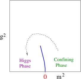
Figure 12: Complementarity: In a gauge theory (coupling $g$) with scalars (mass $m^{2}$) in the fundamental representation, Fradkin and Shenker have shown[87] that the confining and Higgs phases can be smoothly connected. This implies that the massless spectrum is the same in both phases.

Note that, in the Higgs phase picture, the condensate $\langle\chi\psi\rangle$ transforms in the fundamental representation of the gauge group. Fradkin and Shenker have shown[87] that in a gauge theory with scalars transforming in the fundamental representation, the confining and Higgs phases are smoothly connected (see fig. 12). This implies that the massless spectrum is the same in both phases. The behavior we have noted in the chiral $SU(5)$ gauge theory is a dynamical realization of complementarity.

7.3 Mooses[88, 89]

Georgi has proposed a class of composite models with QCD-like dynamics. The models are most easily described diagrammatically (‘‘moose’’ diagrams), with the basic element

(106)

where the solid circle denotes an $SU(N)$ gauge group, the dashed circle an $SU(M)$ global group, and the line a left-handed $(N,\bar{M})$ fermion. In this notation, QCD with three light flavors is

(107)

where the global $SU(3)_{L}\times SU(3)_{R}$ are shown by the outer circles and $SU(3)_{C}$ by the middle circle. The fermions $(3,\bar{3},1)_{+1}$ are denoted by the left-hand line, and $(1,3,\bar{3})_{-1}$ by the right-hand one. Finally, the charges for the non-anomalous $U(1)_{B}$ are shown by the numbers above the line. The constraints of anomaly cancellation are easily seen: gauge anomalies are canceled whenever the number of lines leaving a solid circle equal the number of lines entering; nonanomalous global $U(1)$’s exist if the total charge of the fermions coupled to a given gauge group equals zero. After QCD chiral symmetry breaking, the fermions condense and the residual global symmetries ‘‘collapse’’ the moose diagram to

(108)

which denotes the residual vector $SU(3)$ symmetry.

The simplest nontrivial model of this sort is the ‘‘odd linear moose’’

(109)

which has an $SU(M)\times SU(N)\times U(1)$ global symmetry. Assuming both gauge groups confine, all global anomalies are saturated by a massless $\psi_{\alpha}\psi_{\beta}\psi_{\gamma}$ bound state with quantum numbers $(M,\bar{N})_{+1}$.

The odd linear moose has two complementary Higgs phase pictures depending on the scales, $\Lambda_{SU(M)}$ and $\Lambda_{SU(N)}$, at which the two gauge groups become strong. If $\Lambda_{SU(N)}\gg\Lambda_{SU(M)}$, $SU(N)$ behaves like QCD and the symmetry breaking pattern $SU(M)_{global}\times SU(M)_{gauge}\to SU(M)_{global}$ is expected. In this case a $\psi_{\alpha}\psi_{\beta}$ dynamical mass forms and the remaining $\psi_{\gamma}$ is massless. Alternatively, if $\Lambda_{SU(M)}\gg\Lambda_{SU(N)}$, the symmetry breaking $SU(N)_{global}\times SU(N)_{gauge}\to SU(N)_{global}$ is expected, a $\psi_{\beta}\psi_{\gamma}$ dynamical mass forms, and $\psi_{\alpha}$ remains massless. In all cases a massless $(M,\bar{N})_{+1}$ fermion remains, summarized by the ‘‘reduced moose’’

$$\includegraphics*[width=56.9055pt]{figures/twoglobal.eps}~{}.$$ (110)

Out of these basic ingredients, many models[88, 89] with composite fermions (and scalars) can be formed, and the interested reader is encouraged to explore the literature.

8 Composite Gauge Bosons: Duality in SUSY $SU(N_{c})$

Consider a supersymmetric $SU(N_{c})$ gauge theory with $N_{f}$ flavors. The left-handed fermions $\psi_{L}$, of an ordinary gauge theory, become ‘‘chiral superfields’’ comprised of a complex scalar $Q$ and left-handed fermion $\psi_{Q}$. Similarly, the left-handed charge conjugate fermions of an ordinary gauge theory $\psi^{c}_{L}$ become the fields $\bar{Q}$ and $\psi_{\bar{Q}}$. The gluon $g$ of the ordinary theory becomes a ‘‘vector superfield’’ with the addition of the gluino, an adjoint Majorana-Weyl fermion $\lambda^{a}$ ($\lambda_{L}\equiv\lambda^{c}_{R}$). The global symmetry of the theory is $SU(N_{f})_{L}\times SU(N_{f})_{R}\times U(1)_{B}\times{U(1)_{R}}$, where the fermions have charges

$$\begin{array}[]{c|c|cccc}&SU(N_{c})&SU(N_{f})_{L}&SU(N_{f})_{R}&U(1)_{B}&U(1)_{R}\\ \hline\cr\psi_{Q}&N_{c}&N_{f}&1&1&-\,{N_{c}\over N_{f}}\\ \psi_{\bar{Q}}&\bar{N_{c}}&1&\bar{N_{f}}&-1&-\,{N_{c}\over N_{f}}\\ \lambda&N^{2}_{c}-1&1&1&0&+1\\ \end{array}$$ (111)

Note that the addition of the massless gluinos has resulted in an additional nonanomalous symmetry $U(1)_{R}$. The anomaly factor for $U(1)_{R}SU(N_{c})^{2}$ is

$$2\cdot N_{f}\cdot\left(-{N_{c}\over N_{f}}\right){1\over 2}+(+1)N_{c}\equiv 0$$ (112)

where we note that the index of the fundamental is $1/2$ while that of the adjoint is $N_{c}$.

Seiberg[91] has conjectured that, for $N_{c}+1<N_{f}<3N_{c}$, this theory is a ‘‘dual’’, i.e. has the same low-energy theory as, a supersymmetric $SU(N_{f}-N_{c})$ gauge theory with fields

$$\begin{array}[]{c|c|cccc}&SU(N_{f}-N_{c})&SU(N_{f})_{L}&SU(N_{f})_{R}&U(1)_{B}&U(1)_{R}\\ \hline\cr\psi_{q}&N_{f}-N_{c}&\overline{N_{f}}&1&{N_{c}\over{N_{f}-N_{c}}}&{N_{c}\over N_{f}}-1\\ \psi_{\bar{q}}&\overline{N_{f}-N_{c}}&1&N_{f}&-{N_{c}\over{N_{f}-N_{c}}}&{N_{c}\over N_{f}}-1\\ \psi_{M}&0&N_{f}&\overline{N_{f}}&0&1-{2N_{c}\over N_{f}}\\ \tilde{\lambda}&(N_{f}-N_{c})^{2}-1&1&1&0&+1\\ \end{array}$$ (113)

and a superpotential $W\propto M\psi_{q}\psi_{\bar{q}}$ coupling the global symmetries on the dual ‘‘quark’’ $q$ and ‘‘meson’’ $M$ fields.

All global anomalies match, but only if both the mesons and dual gauginos are included! Unlike the composite theories we have discussed previously, the dual gauge bosons and quarks cannot be interpreted as simple bound states of fundamental particles. The proposed duality satisfies[90] a number of other nontrivial checks as well, including: holomorphic decoupling, consistency with non-abelian conformal phase $3N_{c}/2<N_{f}<3N_{c}$, generalization to $N=2$ supersymmetric theories and string calculations. While no proof has yet been given, the overwhelming preponderance of evidence indicates that Seiberg duality holds and the theory described provides a highly nontrivial example of compositeness.

For your consideration …

Verify that all of the following $SU(N_{c})$ anomalies match in the $SU(N_{f}-N_{c})$ dual theory:

• $(SU(N_{f})_{L})^{3}$

• $(SU(N_{f})_{L})^{2}U(1)_{B}$

• $(SU(N_{f})_{L})^{2}U(1)_{R}$

• $(U(1)_{B})^{2}U(1)_{R}$

• ${\rm Tr}\,U(1)_{R}$ (‘‘gravitational anomaly’’)

• $(U(1)_{R})^{3}$

9 The ACS Conjecture[92]

Given the panoply of examples we have considered, it is worth asking if there is a limit on the complexity of the low-energy theory. Consider the free-energy per unit volume ${\cal F}$ of a theory at temperature $T$, and define

$$f_{IR}=-\lim_{T\to 0}{{\cal F}\over T^{4}}{90\over\pi^{2}}$$ (114)

and

$$f_{UV}=-\lim_{T\to\infty}{{\cal F}\over T^{4}}{90\over\pi^{2}}~{}.$$ (115)

For a free theory, both equal $n_{B}+{7n_{F}/8}$. In this sense, $f_{IR,UV}$ counts the number of low- and high-energy degrees of freedom. Appelquist, Cohen, and Schmaltz have conjectured[92] that:

$$f_{IR}\leq f_{UV}~{},$$ (116)

corresponding to the intuitively reasonable result that the number of degrees of freedom should not increase at low energies. This conjecture has been confirmed for a number of models,[92, 93] but no general proof has been found.

10 Conclusions on Compositeness

• Experimental limits place a lower bound of order 4 TeV (using the ELP[54] convention) on the scale of quark and lepton compositeness.

• Weak coupling and asymptotic freedom imply that the standard model gauge bosons are likely to be fundamental; the longitudinal $W$ and $Z$ may be composite with a scale of order 1 TeV or higher.

• Composite Scalars: Generically, light scalars occur near a 2nd order phase transition. ‘‘Tuning’’ is required to keep them light compared to the compositeness scale, leading to potential hierarchy/naturalness problems!

• Composite Fermions: Massless fermions are a natural consequence of confinement and unbroken chiral symmetry. ’t Hooft’s anomaly matching conditions must be satisfied.

• Composite Gauge Bosons: Seiberg duality shows 4-dimensional field theory at its most subtle -- who says we need 10 or 11 dimensions!

Acknowledgements:

I thank Jon Rosner and K. T. Mahanthappa for organizing a stimulating summer school, and Gustavo Burdman, Myckola Schwetz, and especially Elizabeth Simmons for comments on the manuscript. This work was supported in part by the Department of Energy under grant DE-FG02-91ER40676.

References

- [1] R. S. Chivukula, (1998), hep-ph/9803219.
- [2] D. E. Groom et al., Eur. Phys. J. C15, 1 (2000).
- [3] S. Weinberg, Phys. Rev. D19, 1277 (1979).
- [4] L. Susskind, Phys. Rev. D20, 2619 (1979).
- [5] M. Weinstein, Phys. Rev. D8, 2511 (1973).
- [6] P. Sikivie, L. Susskind, M. Voloshin, and V. Zakharov, Nucl. Phys. B173, 189 (1980).
- [7] E. Eichten and K. Lane, Phys. Lett. 90B, 125 (1980).
- [8] S. Dimopoulos and L. Susskind, Nucl. Phys. B155, 237 (1979).
- [9] S. Weinberg, Physica 96A, 327 (1979).
- [10] H. Georgi, Menlo Park, Usa: Benjamin/cummings ( 1984) 165p.
- [11] A. Manohar and H. Georgi, Nucl. Phys. B234, 189 (1984).
- [12] J. Gasser and H. Leutwyler, Nucl. Phys. B250, 465 (1985).
- [13] E. Farhi and L. Susskind, Phys. Rev. D20, 3404 (1979).
- [14] R. S. Chivukula and H. Georgi, Phys. Lett. 188B, 99 (1987).
- [15] R. Dashen, Phys. Rev. 183, 1245 (1969).
- [16] R. D. Peccei and H. R. Quinn, Phys. Rev. Lett. 38, 1440 (1977).
- [17] R. D. Peccei and H. R. Quinn, Phys. Rev. D16, 1791 (1977).
- [18] S. Weinberg, Phys. Rev. Lett. 40, 223 (1978).
- [19] F. Wilczek, Phys. Rev. Lett. 40, 279 (1978).
- [20] K. Lane, (1993), hep-ph/9401324.
- [21] T. Appelquist, M. J. Bowick, E. Cohler, and A. I. Hauser, Phys. Rev. Lett. 53, 1523 (1984).
- [22] T. Appelquist, M. J. Bowick, E. Cohler, and A. I. Hauser, Phys. Rev. D31, 1676 (1985).
- [23] R. S. Chivukula, S. B. Selipsky, and E. H. Simmons, Phys. Rev. Lett. 69, 575 (1992), hep-ph/9204214.
- [24] L. Randall and R. Sundrum, Phys. Lett. B312, 148 (1993), hep-ph/9305289.
- [25] B. Holdom, Phys. Rev. D24, 1441 (1981).
- [26] B. Holdom, Phys. Lett. 150B, 301 (1985).
- [27] K. Yamawaki, M. Bando, and K. iti Matumoto, Phys. Rev. Lett. 56, 1335 (1986).
- [28] T. W. Appelquist, D. Karabali, and L. C. R. Wijewardhana, Phys. Rev. Lett. 57, 957 (1986).
- [29] T. Appelquist and L. C. R. Wijewardhana, Phys. Rev. D35, 774 (1987).
- [30] T. Appelquist and L. C. R. Wijewardhana, Phys. Rev. D36, 568 (1987).
- [31] H. Pagels, Phys. Rept. 16, 219 (1975).
- [32] M. E. Peskin, Lectures presented at the Summer School on Recent Developments in Quantum Field Theory and Statistical Mechanics, Les Houches, France, Aug 2 - Sep 10, 1982.
- [33] R. Fukuda and T. Kugo, Nucl. Phys. B117, 250 (1976).
- [34] K. Higashijima, Phys. Rev. D29, 1228 (1984).
- [35] K. Lane, Phys. Rev. D10, 2605 (1974).
- [36] H. D. Politzer, Nucl. Phys. B117, 397 (1976).
- [37] J. M. Cornwall, R. Jackiw, and E. Tomboulis, Phys. Rev. D10, 2428 (1974).
- [38] T. Appelquist, K. Lane, and U. Mahanta, Phys. Rev. Lett. 61, 1553 (1988).
- [39] A. Cohen and H. Georgi, Nucl. Phys. B314, 7 (1989).
- [40] U. Mahanta, Phys. Rev. Lett. 62, 2349 (1989).
- [41] M. E. Peskin and T. Takeuchi, Phys. Rev. Lett. 65, 964 (1990).
- [42] M. E. Peskin and T. Takeuchi, Phys. Rev. D46, 381 (1992).
- [43] M. Golden and L. Randall, Nucl. Phys. B361, 3 (1991).
- [44] B. Holdom and J. Terning, Phys. Lett. B247, 88 (1990).
- [45] A. Dobado, D. Espriu, and M. J. Herrero, Phys. Lett. B255, 405 (1991).
- [46] H. Georgi, Ann. Rev. Nucl. Part. Sci. 43, 209 (1993).
- [47] D. B. Kaplan, (1995), nucl-th/9506035.
- [48] A. Pich, (1998), hep-ph/9806303.
- [49] H. Georgi, Phys. Lett. B298, 187 (1993), hep-ph/9207278.
- [50] R. S. Chivukula, M. J. Dugan, and M. Golden, Phys. Lett. B292, 435 (1992), hep-ph/9207249.
- [51] A. G. Cohen, D. B. Kaplan, and A. E. Nelson, Phys. Lett. B412, 301 (1997), hep-ph/9706275.
- [52] S. Coleman, J. Wess, and B. Zumino, Phys. Rev. 177, 2239 (1969).
- [53] J. Curtis G. Callan, S. Coleman, J. Wess, and B. Zumino, Phys. Rev. 177, 2247 (1969).
- [54] E. Eichten, K. Lane, and M. E. Peskin, Phys. Rev. Lett. 50, 811 (1983).
- [55] S. Weinberg, Phys. Rev. 135, B1049 (1964).
- [56] LEP Electroweak Working Group, http://lepewwg.web.cern/LEPEWWG/tgc/.
- [57] K. Hagiwara, R. D. Peccei, D. Zeppenfeld, and K. Hikasa, Nucl. Phys. B282, 253 (1987).
- [58] S. Weinberg and E. Witten, Phys. Lett. B96, 59 (1980).
- [59] V. A. Miranskii, M. Tanabashi, and K. Yamawaki, Mod. Phys. Lett. A4, 1043 (1989).
- [60] V. A. Miranskii, M. Tanabashi, and K. Yamawaki, Phys. Lett. B221, 177 (1989).
- [61] Y. Nambu, Enrico Fermi Institute - EFI-89-08.
- [62] W. J. Marciano, Phys. Rev. Lett. 62, 2793 (1989).
- [63] W. A. Bardeen, C. T. Hill, and M. Lindner, Phys. Rev. D41, 1647 (1990).
- [64] C. T. Hill, Phys. Lett. B266, 419 (1991).
- [65] G. Cvetic, (1997), hep-ph/9702381.
- [66] B. A. Dobrescu and C. T. Hill, Phys. Rev. Lett. 81, 2634 (1998), hep-ph/9712319.
- [67] R. S. Chivukula, B. A. Dobrescu, H. Georgi, and C. T. Hill, Phys. Rev. D59, 075003 (1999), hep-ph/9809470.
- [68] C. T. Hill, Phys. Lett. B345, 483 (1995), hep-ph/9411426.
- [69] Y. Nambu and G. Jona-Lasinio, Phys. Rev. 122, 345 (1961).
- [70] R. S. Chivukula, (2000), hep-ph/0005168.
- [71] K. G. Wilson, Phys. Rev. B4, 3174 (1971).
- [72] K. G. Wilson, Phys. Rev. B4, 3184 (1971).
- [73] K. G. Wilson and J. Kogut, Phys. Rept. 12, 75 (1974).
- [74] J. Kuti, L. Lin, and Y. Shen, Phys. Rev. Lett. 61, 678 (1988).
- [75] W. Buchmuller and D. Wyler, Nucl. Phys. B268, 621 (1986).
- [76] B. Grinstein and M. B. Wise, Phys. Lett. B265, 326 (1991).
- [77] R. S. Chivukula and E. H. Simmons, Phys. Lett. B388, 788 (1996), hep-ph/9608320.
- [78] R. S. Chivukula, C. Holbling, and N. Evans, Phys. Rev. Lett. 85, 511 (2000), hep-ph/0002022.
- [79] LEP Electroweak Working Group, http://lepewwg.web.cern.ch/LEPEWWG/plots/summer2000/.
- [80] D. Amidei and R. Brock, http://fnalpubs.fnal.gov/archive/1996/pub/Pub-96-082.ps.
- [81] G. ’t Hooft and others (ed.), New York, Usa: Plenum ( 1980) 438 P. ( Nato Advanced Study Institutes Series: Series B, Physics, 59).
- [82] J. S. Bell and R. Jackiw, Nuovo Cim. A60, 47 (1969).
- [83] S. L. Adler, Phys. Rev. 177, 2426 (1969).
- [84] R. Jackiw and K. Johnson, Phys. Rev. 182, 1459 (1969).
- [85] J. Schwinger, Phys. Rev. 82, 664 (1951).
- [86] G. ’t Hooft, Phys. Rev. Lett. 37, 8 (1976).
- [87] E. Fradkin and S. H. Shenker, Phys. Rev. D19, 3682 (1979).
- [88] H. Georgi, Nucl. Phys. B266, 274 (1986).
- [89] H. Georgi, Harvard Univ. Cambridge - HUTP-86-A040.
- [90] M. E. Peskin, (1997), hep-th/9702094.
- [91] N. Seiberg, Nucl. Phys. B435, 129 (1995), hep-th/9411149.
- [92] T. Appelquist, A. G. Cohen, and M. Schmaltz, Phys. Rev. D60, 045003 (1999), hep-th/9901109.
- [93] T. Appelquist, A. Cohen, M. Schmaltz, and R. Shrock, Phys. Lett. B459, 235 (1999), hep-th/9904172.