Abstract

The renormalization group evolution equation for two neutrino mixing is known to exhibit nontrivial fixed point structure corresponding to maximal mixing at the weak scale. The presence of the fixed point provides a natural explanation of the observed maximal mixing of $\nu_{\mu}-\nu_{\tau}$ if the $\nu_{\mu}$ and $\nu_{\tau}$ are assumed to be quasi-degenerate at the seesaw scale without constraining on the mixing angles at that scale. In particular, it allows them to be similar to the quark mixings as in generic grand unified theories. We discuss implementation of this program in the case of MSSM and find that the predicted mixing remains stable and close to its maximal value, for all energies below the $O$(TeV) SUSY scale. We also discuss how a particular realization of this idea can be tested in neutrinoless double beta decay experiments.

PACS numbers: 12.15.Ff, 12.60.-i

I INTRODUCTION

Theoretical understanding of experimentally measured neutrino anomalies poses a major challenge to unified gauge theories especially since $\nu_{\mu}-\nu_{\tau}$ mixing has been observed to be close to maximal through atmospheric neutrino flux measurements whereas the mixing in the corresponding quark sector is small. The problem is so severe that, only over the limited span of the last two years, nearly a hundred models have been proposed where considerable effort has been devoted to accommodate large neutrino mixing [1]. There are also interesting suggestions to understand this large mixing in the context of various grand unified theories including $SO(10)$ [2, 3], which unify both quarks and leptons. It is however fair to say that no convincing and widely accepted natural model has yet emerged.

With a view to simplifying model building, we recently suggested criteria for radiative magnification of neutrino mixing[4, 5] which allow a small mixing at high scale to be amplified to large mixing at the weak scale after renormalization group evolution. The only condition that needs to be fulfilled is that the $\nu_{\mu}$ and $\nu_{\tau}$ be quasi-degenerate in mass, as for example would be independently required if LSND results are confirmed. In such models, there is no need to impose special constraints on the theory at high scale beyond those needed to guarantee the quasi-degeneracy. They would, therefore, require less theoretical input compared to the case where one tries to obtain both degeneracy (should it be phenomenologically warranted) and maximal mixing at the high (seesaw) scale within the framework of quark lepton unification.

A key role in the above scenario is played by the renormalization group equations for neutrino masses and mixings [6, 7]. In this paper, we exploit one of the most interesting and highly appealing aspect of renormalisation group (RG) running of gauge and Yukawa couplings i.e. the emergence of fixed point (FP) structure. Use of FP structure of RGE’s to understand low energy parameters is not new; for example, it is often invoked [8] to understand the top quark mass at the weak scale starting with a wider range of possible values at the GUT scale as would be preferred by the naturalness requirement in GUT theories.

It was noted in [6] that neutrino mixings can have fixed points corresponding to maximal mixing and several examples were given to illustrate this point in the standard model and two Higgs model. The desirable value of $\sin^{2}(2\theta)\sim 1$ were shown to arise in these models both at the electroweak and at intermediate scales of order $10^{8}$ GeV or so depending on the model parameters at the high scale. Our goal in the present work is to extend the discussion of [6] to supersymmetric theories (MSSM) and delineate the constraints on the high scale theory under which the fixed point (or maximal mixing) occurs around the weak scale. We discuss the conditions under which the value of the mixing remains stable as the energy is varied from TeV to $M_{Z}$ scale. A crucial requirement for the fixed point to occur is that the muon and the tau neutrinos must be quasi-degenerate. Our analysis further clarifies the idea of radiative magnification discussed in Ref.[4, 5]. We the point out that in a special class of models which extend this idea to the case of three degenerate neutrinos, then searches for neutrinoless double beta decay can provide a test of these models.

The paper is organised as follows. In section II, we discuss radiative correction and derivation of RGEs for mixing angle in the standard model (SM) and minimal supersymmetric standard model (MSSM). In section III, we obtain analytic solution for the RGE and demonstrate explicitly the renormalisation group fixed point (RGFP) structure. In section IV, we show how the FP occurs naturally at the weak scale for quasidegenerate neutrinos leading to the condition of radiative magnification. We also derive a new stability criterion and show how the FP and magnification occur in MSSM starting from small mixings as in the quark sector. In section V, we comment on tests of the radiative magnification scheme in neutrinoless double beta decay searches.

II Radiative Corrections and RGE for Neutrino Mixing

In both SM and MSSM, we consider radiative corrections in the flavor basis to the light Majorana neutrino mass matrix, $m_{\alpha\beta}$, which is a 5-dim operator scaled by the high mass, $M_{N}$ (e.g. see-saw or R.H. Majorana neutrino mass scale), where the mass matrix is generated, with

$${\cal L}_{\nu\nu}=-\nu_{\alpha}^{T}C^{-1}m_{\alpha_{\beta}}\nu_{\beta}+{\rm h.c..}$$ (1)

As a result of one-loop radiative corrections the RGEs below $\mu=M_{N}$ are [6, 7]

SM

$$16\pi^{2}{dm\over dt} = \left[-3g_{2}^{2}+2\lambda+{\rm Tr}\left(6Y_{U}^{\dagger}Y_{U}+6Y_{D}^{\dagger}Y_{D}+2Y_{E}^{\dagger}Y_{E}\right)\right]m$$ (2)

$$- {1\over 2}\left[m\left(Y_{E}Y_{E}^{\dagger}\right)+\left(Y_{E}Y_{E}^{\dagger}\right)^{T}m\right]~{}.$$ (3)

MSSM

$$16\pi^{2}{dm\over dt}=\left[-{6\over 5}g_{1}^{2}-6g_{2}^{2}+{\rm Tr}\left(6Y_{U}^{\dagger}Y_{U}\right)\right]m+\left[m\left(Y_{E}Y_{E}^{\dagger}\right)+\left(Y_{E}Y_{E}^{\dagger}\right)^{T}m\right]~{}.$$ (4)

In (3) and (4) $g_{1}(g_{2})$ are the $U(1)_{Y}(SU(2)_{L})$ gauge couplings, $\lambda$ is the Higgs quartic coupling (in SM), whereas $Y_{U}(Y_{D})$ and $Y_{E}$ are the Yukawa matrices for the up(down) quarks and charged leptons. We work in the charged lepton diagonal basis where the unitary matrix $U_{\alpha i}$ that transforms mass basis to flavor basis is identified as the standard MNS matrix [9]. Using (3) and (4), the mass matrix is evolved from the high scale down to $t(=\ln\mu)<t_{0}(=\ln M_{N})$ in the SM or MSSM.

SM

$$m(\mu)=\left({\mu\over M_{N}}\right)^{\left(\lambda\over 16\pi^{2}\right)}I^{-3}_{g_{2}}I^{6}_{\rm top}I^{3}_{b}I_{\tau}\times\left[\begin{array}[]{ccc}m_{ee}^{0}I^{\prime}_{e}&m_{e\mu}^{0}\sqrt{I^{\prime}_{e}I^{\prime}_{\mu}}&m_{e\tau}^{0}\sqrt{I^{\prime}_{e}I^{\prime}_{\tau}}\\ m_{\mu e}^{0}\sqrt{I^{\prime}_{e}I^{\prime}_{\mu}}&m_{\mu\mu}^{0}I^{\prime}_{\mu}&m_{\mu\tau}^{0}\sqrt{I^{\prime}_{\mu}I^{\prime}_{\tau}}\\ m_{\tau e}^{0}\sqrt{I^{\prime}_{e}I^{\prime}_{\tau}}&m_{\tau\mu}^{0}\sqrt{I^{\prime}_{\mu}I^{\prime}_{\tau}}&m_{\tau\tau}^{0}I^{\prime}_{\tau}\end{array}\right]~{}.$$ (5)

MSSM

$$m(\mu)=I_{g_{1}}^{-6\over 5}I^{-6}_{g_{2}}I^{6}_{\rm top}\times\left[\begin{array}[]{ccc}m_{ee}^{0}I^{2}_{e}&m_{e\mu}^{0}I_{e}I_{\mu}&m_{e\tau}^{0}I_{e}I_{\tau}\\ m_{\mu e}^{0}I_{e}I_{\mu}&m_{\mu\mu}^{0}I^{2}_{\mu}&m_{\mu\tau}^{0}I_{\mu}I_{\tau}\\ m_{\tau e}^{0}I_{e}I_{\tau}&m_{\tau\mu}^{0}I_{\mu}I_{\tau}&m_{\tau\tau}^{0}I^{2}_{\tau}\end{array}\right]~{}.$$ (6)

Here,

$$I_{h}(\equiv{I^{\prime}_{h}}^{-1})=e^{\delta_{h}}=\exp\left({1\over 8\pi^{2}}\int_{t_{0}}^{t}h^{2}(t^{\prime})dt^{\prime}\right)~{},$$ (7)

and $h$ denotes the gauge coupling $(g_{1},g_{2})$ or the Yukawa-coupling-eigen value for quarks and charged leptons $(y_{\rm top},y_{b},y_{\tau},y_{\mu},y_{e})$. When the running VEV of the up-type Higgs doublet in MSSM is taken into account the common factor in (6) is changed with the replacement, $I_{g_{1}}^{-6/5}I_{g_{2}}^{-6}I_{\rm top}^{6}\to I_{g_{1}}^{-9/10}I_{g_{2}}^{-9/2}$ and similarly in SM. In subsequent discussions for mixing angle we ignore common renormalisation factors in (5) and (6) as they cancel out in the relevant expressions. At any value of $t<t_{0}$,

$$\tan 2\theta(t)={2m_{\mu\tau}(t)\over m_{\tau\tau}(t)-m_{\mu\mu}(t)}~{},$$ (8)

and (3), (4), and (8) give the RGEs for $\sin^{2}(2\theta)$,

SM

$$16\pi^{2}{d\sin^{2}2\theta\over dt} = \sin^{2}2\theta\cos^{2}2\theta\left(y_{\tau}^{2}-y_{\mu}^{2}\right){m_{\tau\tau}+m_{\mu\mu}\over m_{\tau\tau}-m_{\mu\mu}}$$ (9)

$$= \sin^{2}2\theta{\left(m_{\tau\tau}^{2}-m_{\mu\mu}^{2}\right)\left(y^{2}_{\tau}-y^{2}_{\mu}\right)\over\left(m_{\tau\tau}-m_{\mu\mu}\right)^{2}+4m_{\mu\tau}^{2}}~{}.$$ (10)

MSSM

$$16\pi^{2}{d\sin^{2}2\theta\over dt} = -2\sin^{2}2\theta\cos^{2}2\theta\left(y_{\tau}^{2}-y_{\mu}^{2}\right){m_{\tau\tau}+m_{\mu\mu}\over m_{\tau\tau}-m_{\mu\mu}}$$ (11)

$$= -2\sin^{2}2\theta{\left(m_{\tau\tau}^{2}-m_{\mu\mu}^{2}\right)\left(y^{2}_{\tau}-y^{2}_{\mu}\right)\over\left(m_{\tau\tau}-m_{\mu\mu}\right)^{2}+4m_{\mu\tau}^{2}}~{}.$$ (12)

All quantities in the RHS of (10) and (12) are $t$-dependent. As was noted in [6], both the RGEs have one trivial fixed point at $\sin^{2}2\theta=0$ and the other nontrivial fixed point at $\sin^{2}2\theta=1$. Recently the FP structure of MNS matrix has been also investigated in [10]. Assuming that the initial high-scale texture of the mass matrix is such that the nontrivial fixed point occurs at a scale $\mu_{c}(M_{Z}\leq\mu_{c}<M_{N},t_{c}=\ln\mu_{c})$, we have the FP condition,

$$\sin^{2}2\theta(t_{c})=1~{},$$ (13)

or, equivalently,

$$m_{\tau\tau}(t_{c})=m_{\mu\mu}(t_{c})~{}.$$ (14)

III Analytic Formula and Fixed Point

Before obtaining analytic solutions to (10) and (12), it is worthwhile to explain why resonance structures in the numerical solutions [6, 10, 11, 12] in the $\sin^{2}2\theta(t)$ vs. $t$ plots are expected for specific textures of $m^{0}_{\alpha\beta}$.

Noting that,

$$\left|y_{\tau}(t)\right|^{2}\gg\left|y_{\mu}(t)\right|^{2}$$ (15)

(6) states that in MSSM, as $t$ decreases below $t_{0}$, the ratio, $R_{\tau}(t)=m_{\tau\tau}(t)/m_{\tau\tau}^{0}$, decreases faster from its high scale value, $(R_{\tau}(t_{0})=1)$, as compared to the rate of decrease of the ratio, $R_{\mu}(t)=m_{\mu\mu}(t)/m_{\mu\mu}^{0}$. In particular, the relations (13) and (14) are satisfied at $t=t_{c}$ if

$$m_{\tau\tau}^{0}e^{2\delta_{\tau}(t_{c})}=m_{\mu\mu}^{0}~{}.$$ (16)

For the FP to occur at $t_{c}<t_{0}$, the high scale texture must be such that $m_{\tau\tau}^{0}$ and $m_{\mu\mu}^{0}$ are comparable but unequal with $m_{\tau\tau}^{0}>m_{\mu\mu}^{0}$. Lower values of $t_{c}$ corresponds to larger differences between $m_{\tau\tau}^{0}$ and $m_{\mu\mu}^{0}$.

From (12) it is clear that when $m_{\tau\tau}(t_{c})=m_{\mu\mu}(t_{c})$, the slope of the curve in the $\sin^{2}2\theta(t)$ vs. $t$ plot vanishes at $t=t_{c}$. For $t>t_{c}$, $m_{\tau\tau}(t)>m_{\mu\mu}(t)$, the slope is negative; but for $t<t_{c}$, $m_{\tau\tau}(t)<m_{\mu\mu}(t)$ and the slope is positive as given by the RGE. Negative(positive) slope to the right(left) with vanishing slope at $t=t_{c}$ is the characteristic feature of a resonance curve as predicted by (12) for MSSM. Similar result emerges for SM from (10) with somewhat different high-scale condition with $m_{\mu\mu}^{0}>m_{\tau\tau}^{0}$ and the ratios $R_{\tau}(t)$ and $R_{\mu}(t)$ increase as $t$ decreases below $t_{0}$. Thus it is clear that for certain given textures at high scale $(m_{\mu\mu}^{0},m_{\tau\tau}^{0}$ and $m_{\mu\tau}^{0})$ resonance occurs at $t=t_{c}$ converting small mixing at high scale to large mixing at lower scales.

Inspite of the terse nature of the RHS of (12), using the almost exact approximation, $|\delta_{\tau}(t)|\gg|\delta_{\mu}(t)|$, we have integrated it to obtain analytic solution for RG evolution of $\sin^{2}2\theta$ in the MSSM for all values of $\mu<M_{N}$,

$$\sin^{2}2\theta(t)=\sin^{2}2\theta_{0}{\left[\left(m_{\tau\tau}^{0}-m_{\mu\mu}^{0}\right)^{2}+4{m_{\mu\tau}^{0}}^{2}\right]e^{2\delta_{\tau}(t)}\over\left[\left(m_{\tau\tau}^{0}e^{2\delta_{\tau}(t)}-m_{\mu\mu}^{0}\right)^{2}+4{m_{\mu\tau}^{0}}^{2}e^{2\delta_{\tau}(t)}\right]}~{},$$ (17)

where, $\theta_{0}$, is the high scale mixing angle with

$$\tan 2\theta_{0}={2m_{\mu\tau}^{0}\over\left(m_{\tau\tau}^{0}-m_{\mu\mu}^{0}\right)}~{}.$$ (18)

Given,

$$m_{\mu\mu}(t)/m_{\tau\tau}(t) = (m_{\mu\mu}^{0}/m_{\tau\tau}^{0})e^{2\delta_{\mu}(t)}e^{-2\delta_{\tau}(t)}~{},$$ (19)

$$m_{\mu\tau}(t)/m_{\tau\tau}(t) = (m_{\mu\tau}^{0}/m_{\tau\tau}^{0})e^{\delta_{\mu}(t)}e^{-\delta_{\tau}(t)}~{},$$ (20)

and using (6)-(8), (17) may be recognised as the approximation, $|\delta_{\mu}(t)|\ll|\delta_{\tau}(t)|$, to the following exact analytic solution of (12),

$$\sin^{2}2\theta(t)=\sin^{2}2\theta_{0}{\left[\left(m_{\tau\tau}^{0}-m_{\mu\mu}^{0}\right)^{2}+4{m_{\mu\tau}^{0}}^{2}\right]e^{2\delta_{\tau}(t)}e^{2\delta_{\mu}(t)}\over\left[\left(m_{\tau\tau}(t)-m_{\mu\mu}(t)\right)^{2}+4m_{\mu\tau}(t)^{2}\right]}~{}.$$ (21)

Replacing $\theta(t)\to\theta(\mu)$, $m_{ij}(t)\to m_{ij}(\mu)$, $\theta_{0}\to\theta(M)$, and $m_{ij}^{0}\to m_{ij}(M)$, formulas (17) or (21) can be used to derive $\theta(\mu)$ from $\theta(M)$ or vice versa for all values of $\mu<M\leq M_{N}$. It is interesting to note that these analytic solutions exhibit both the resonance as well as the nontrivial FP structure explicitly. While detailed features of resonance such as the $t$-dependent width, maximal mixing at the peak, and smaller mixings for $t>t_{c}$ or $t<t_{c}$ are clearly exhibited, the FP structure is proved as follows. At $t=t_{c}$, when (14) or (16) are satisfied, the quantity inside the parenthesis in the denominator of (21) or (17) vanishes. Then using (18), (17) and (21) give

$$\sin^{2}2\theta(t_{c})=\sin^{2}2\theta_{0}\left[{\left(m_{\tau\tau}^{0}-m_{\mu\mu}^{0}\right)^{2}\over{4m_{\mu\tau}^{0}}^{2}}+1\right]=\sin^{2}2\theta_{0}+\cos^{2}2\theta_{0}=1~{}.$$ (22)

It is to be noted that (22) holds for all initial value of $\theta_{0}<\pi/4$, thus demonstrating the fixed point behavior corresponding to maximal mixing. Although the relation (22) appears to be true also for $\theta_{0}=\pi/4$ showing that maximal mixing remains maximal at $t=t_{c}$, the RG evolution equations never satisfy $m_{\tau\tau}(t_{c})=m_{\mu\mu}(t_{c})$ for $t_{c}\ll t_{0}$ if we start with the initial condition $m_{\tau\tau}^{0}=m_{\mu\mu}^{0}$ which is necessary for $\theta_{0}=\pi/4$. In fact nearly maximal mixings at the high scale are damped out to small mixings at lower scales $(\mu\ll M_{N})$ due to nonvanishing contributions of the quantity $\left(m_{\tau\tau}(t_{c})-m_{\mu\mu}(t_{c})\right)^{2}$ in the R.H.S. of (17) or (21). Thus the analytic formula, apart from demonstrating the FP structure and resonance behavior, also explains why large mixing at high scales are damped out to small mixings near the weak scale. Also zero mixing angle does not run and continues to be zero down to $\mu=M_{Z}$. Similar analytic solutions are also obtained for SM exhibiting the FP structure with the replacement $2\delta_{i}(t)\to-\delta_{i}(t)$, $i=\mu,\tau$ in (17)-(21).

In almost all cases of RG fixed point discussed so far in the literature, the FP structure is revealed through the differential RGEs and demonstrated through numerical solutions only. But in the present case, apart from the differential RGE and numerical solutions (see section IV), the analytic solutions also exhibit the FP structure explicitly as demonstrated through (17)-(22).

IV Radiative Magnification Through the Fixed Point and Stability

When the condition (13) or (14) is satisfied for $t_{c}=t_{S}=\ln M_{S}$($M_{S}=$SUSY scale), the FP may manifest as large neutrino mixing observed at low energies, for example, in $\nu_{\mu}-\nu_{\tau}$ oscillation scenario necessary to solve the atmospheric neutrino anomaly. In terms of the high scale mass eigen values $(m_{2}^{0},m_{3}^{0})$, mixing angle $(\theta_{0})$, and radiative correction parameters, the condition for FP manifestation at $\mu=\mu_{c}=M_{S}$ then reduces to

$$(m_{2}^{0}-m_{3}^{0})c_{2\theta_{0}}=2\delta_{\tau}(t_{S})\left(m_{2}^{0}s^{2}_{\theta_{0}}+m_{3}^{0}c^{2}_{\theta_{0}}\right)-2\delta_{\mu}(t_{S})\left(m_{2}^{0}c^{2}_{\theta_{0}}+m_{3}^{0}s^{2}_{\theta_{0}}\right)~{}.$$ (23)

where $s_{\theta_{0}}=\sin\theta_{0}$, $c_{\theta_{0}}=\cos\theta_{0}$, $c_{2\theta_{0}}=\cos 2\theta_{0}$ and $s_{2\theta_{0}}=\sin 2\theta_{0}$. Taking $M_{S}=M_{Z}$, this is recognised exactly as the condition that was derived in [4, 5] for magnifying small mixing at high scale to large mixing at low-energies through radiative corrections. But, as noted here, the condition is exact, needs no fine tuning, and emerges as a natural consequence of the manifestation of the FP at the weak scale. For small mixing angles at $\mu=M_{N}$, similar to those existing in the quark sector (e.g. $\theta_{0}\approx V_{cb}\approx 0.04)$, $c_{\theta_{0}}\approx c_{2\theta_{0}}\approx 1$, and $s^{2}_{\theta_{0}}\sim 0$, it is clear that the condition (23) cannot be satisfied if the masses $m_{2}^{0}$ and $m_{3}^{0}$ are hierarchial, or exactly degenerate having the same $(m_{2}^{0}=m_{3}^{0})$ or opposite CP-parity $(m_{2}^{0}=-m_{3}^{0})$. Also it cannot be satisfied if the masses are quasidegenerate with opposite CP-parity $(m_{2}^{0}\sim-m_{3}^{0})$. It can be satisfied only if the masses are quasidegenerate at the high scale having the same CP-parity $(m_{2}^{0}\sim m_{3}^{0})$. Since $\delta_{\tau}$ is negative, a necessary prediction of MSSM is that $m_{3}^{0}>m_{2}^{0}$. In the SM, $2\delta_{\tau}(t_{Z})$ and $2\delta_{\mu}(t_{Z})$ in (23) are replaced by $-\delta_{\tau}(t_{Z})$ and $-\delta_{\mu}(t_{Z})$, respectively, and (23) predicts $m_{2}^{0}>m_{3}^{0}$. These requirements in MSSM or SM are analogous to the occurrence of quasi fixed points in top-quark Yukawa coupling where right order of the top quark mass is obtained only for certain strong interaction couplings. We emphasize that the observed large neutrino mixing in the $\nu_{\mu}-\nu_{\tau}$ sector predicts the corresponding $\nu_{2}(\nu_{3})$ masses to be quasidegenerate with the same CP-parity as a necessary requirement in order that the FP manifests at the lower scale. Under the condition (14), with $t_{c}=t_{S}$, the mass eigen values at $\mu=M_{S}$ are

$$m_{2}(t_{S}) = \left(m_{2}^{0}c_{\theta_{0}}^{2}+m^{0}_{3}s_{\theta_{0}}^{2}\right)(1+2\delta_{\mu}(t_{S}))-(m_{3}^{0}-m_{2}^{0})c_{\theta_{0}}s_{\theta_{0}}(1+\delta_{\tau}(t_{S})+\delta_{\mu}(t_{S}))~{}.$$ (24)

$$m_{3}(t_{S}) = \left(m_{2}^{0}c_{\theta_{0}}^{2}+m^{0}_{3}s_{\theta_{0}}^{2}\right)(1+2\delta_{\mu}(t_{S}))+(m_{3}^{0}-m_{2}^{0})c_{\theta_{0}}s_{\theta_{0}}(1+\delta_{\tau}(t_{S})+\delta_{\mu}(t_{S}))~{}.$$ (25)

Taking the high scale mixings to be small, we obtain the mass squared difference at $\mu=M_{S}$,

$$\Delta m^{2}\equiv m_{3}^{2}-m_{2}^{2}\approx\Delta{m^{0}}^{2}s_{2\theta_{0}}(1+\delta_{\tau}(t_{S}))~{},$$ (26)

where,

$$\Delta{m^{0}}^{2}\approx 2{m_{2}^{0}}^{2}\left(e^{-2\delta_{\tau}(t_{S})}-1\right)\approx-4{m_{2}^{0}}^{2}\delta_{\tau}(t_{S})~{}.$$ (27)

Before proceeding further, we show analytically how the stability of radiative magnification is controlled by the high-scale mixing angle. To generate nearly maximal mixing at a lower scale $(\mu=\mu_{c}=M_{S}=M_{Z})$ starting from small mixing as in the quark sector at the high scale (e.g. $\theta_{0}\approx V_{cb}\approx 0.04$), the FP position is desired to be stable near $M_{S}=M_{Z}$. As the FP is a consequence of radiative corrections, the stability must be guaranteed against smaller changes in the neutrino mass matrix due to higher order corrections. To maintain such stability this requires the mixing to be nearly maximal within at least $\mu\sim$ few $(M_{Z})$. In fact we show that radiative stability is ensured over a larger range. We define the range, $t=t_{S}$ to $t_{\Gamma}$ $(\mu=M_{S}$ to $\mu_{\Gamma})$, within which, the mixing remains nearly maximal. Noting that,

$$\delta_{\tau}(t_{\Gamma})=\delta_{\tau}(t_{S})+\epsilon_{\tau}(t_{\Gamma})~{},$$ (28)

with

$$\epsilon_{\tau}(t_{\Gamma})\approx{y_{\tau}^{2}\over 16\pi^{2}}\ln{\mu_{\Gamma}\over M_{S}}~{},$$ (29)

which remains small $(|\epsilon_{\tau}|\ll 1)$ over a wide range of $y_{\tau}$, we use the FP condition (14) and (16) in (17) and (21) to obtain

$$\sin^{2}2\theta(t_{\Gamma})\approx{1+2\delta_{\tau}(t_{\Gamma})\over\left[1+2\delta_{\tau}(t_{\Gamma})+{{m_{\mu\mu}^{0}}^{2}\over{m_{\mu\tau}^{0}}^{2}}\epsilon^{2}(t_{\Gamma})\right]}~{}.$$ (30)

The stability criterion for the FP position and radiative magnification at $\mu\approx M_{S}$ may be stated as

$${y_{\tau}^{4}{m_{\mu\mu}^{0}}^{2}\over 256\pi^{4}{m_{\mu\tau}^{0}}^{2}}\left(\ln{\mu_{\Gamma}\over M_{S}}\right)^{2}\ll 1~{}.$$ (31)

This clearly has the implication that arbitrarily small values of high-scale mixing cannot maintain a stable FP whereas zero initial mixing continues to remain zero at all lower values of $t$ and is never magnified. For smaller values of $\theta_{0}$ or $m_{\mu\tau}^{0}$, the contribution of the third term in the denominator in (30) becomes larger leading to sharper decrease of the predicted low-scale mixing angle from its maximal fixed point value. This results in the smaller width of the resonance for smaller values of high-scale mixing ($\theta_{0}$ or $m_{\mu\tau}^{0}$). This feature is clearly exhibited through Figs. 1 and 2, where we have presented $\sin 2\theta(\mu)$ for $\mu=100$ GeV-$1$ TeV taking $M_{S}=M_{Z}$, $M_{N}=10^{13}$ GeV, $\tan\beta=50$ and $y_{\tau}=0.49$ with $e^{2\delta_{\tau}(M_{Z})}=0.929$. The high-scale parameters for Fig. 1 are $m_{\tau\tau}^{0}\approx m_{3}^{0}\approx 0.28$ eV, $m_{\mu\mu}^{0}\approx m_{2}^{0}\approx 0.26$ eV, and $m_{\mu\tau}^{0}\approx 0.0044$ eV corresponding to $\theta_{0}=0.22$ consistent with $\Delta m^{2}\approx 4\times 10^{-3}$ eV² needed for atmospheric neutrino data. For Fig. 2 these parameters are $m_{\tau\tau}^{0}\approx m_{3}^{0}\approx 0.27$ eV, $m_{\mu\mu}^{0}\approx m_{2}^{0}\approx 0.25$ eV, and $m_{\mu\tau}^{0}\approx 0.0008$ eV corresponding to $\theta_{0}=V_{cb}=0.04$ consistent with $\Delta m^{2}\approx 7\times 10^{-3}$ eV². It is clear that in Fig. 2 the width is substantially narrower than Fig. 1 and $\sin 2\theta(\mu)$ reduces by nearly $20\%$ from its maximal value over the range of $100-500$ GeV. Such energy dependent mixing between the two neutrinos, as a prediction of MSSM when both the FP and the SUSY scale are at $M_{S}=M_{Z}$ might be possible to testify or falsify in future by high-energy neutrino experiments.

In contrast to the energy dependent mixing discussed above, for the first time we find here a very attractive new feature of the other class of MSSM with higher SUSY scale $M_{S}=O$(TeV) where stable and almost energy independent mixing, close to its maximal value, is predicted over a wider range of energy scale $\mu=M_{Z}$-few TeV starting from the high-scale mixing similar to the quark sector, $\theta_{0}=V_{cb}\approx 0.04$. Using the technique explained above, the high-scale parameters are chosen to have the RG fixed point at the SUSY scale $M_{S}=1$ or few TeV. Then the origin of negligible energy dependence in the predicted mixing at all lower energy scales is explained by noting the nonSUSY SM prediction for which $y_{\tau}\approx 0.01$ below $M_{S}$,

SM: $M_{Z}\leq\mu\leq M_{S}$,

$$\sin^{2}2\theta(\mu) = \sin^{2}2\theta(M_{S}){\left[\left(m_{\tau\tau}(M_{S})-m_{\mu\mu}(M_{S})\right)^{2}+4m_{\mu\tau}^{2}(M_{S})\right]\left({M_{S}\over\mu}\right)^{y_{\tau}^{2}\over 16\pi^{2}}\over\left(m_{\tau\tau}(M_{S})\left({M_{S}\over\mu}\right)^{y_{\tau}^{2}\over 16\pi^{2}}-m_{\mu\mu}(M_{S})\right)^{2}+4m_{\mu\tau}^{2}(M_{S})\left({M_{S}\over\mu}\right)^{y_{\tau}^{2}\over 16\pi^{2}}}$$ (32)

$$= \sin^{2}2\theta(M_{S}){4m_{\mu\tau}^{2}(M_{S})\left({M_{S}\over\mu}\right)^{y_{\tau}^{2}\over 16\pi^{2}}\over m_{\mu\mu}(M_{S})\left(\left({M_{S}\over\mu}\right)^{y_{\tau}^{2}\over 16\pi^{2}}-1\right)^{2}+4m_{\mu\tau}^{2}(M_{S})\left({M_{S}\over\mu}\right)^{y_{\tau}^{2}\over 16\pi^{2}}}~{},$$ (33)

where, (33) has been obtained from (32) by using the FP condition, $m_{\tau\tau}(M_{S})=m_{\mu\mu}(M_{S})$. Then, because of smallness of the $\tau$-Yukawa coupling in the SM with $y_{\tau}\simeq 0.01$ in (33) there is negligible $\mu$-dependence and the predicted mixing remains stable, close to its maximal value, for all values of $\mu$ below $M_{S}=O$(TeV). This behavior is shown in Fig. 3 for initial values of $\theta_{0}=V_{cb}=0.04$, $m_{3}^{0}\approx m_{\tau\tau}^{0}=0.1543$ eV, $m_{2}^{0}\approx m_{\mu\mu}^{0}=0.1434$ eV, $m_{\mu\tau}^{0}=0.00044$ eV, $\Delta m^{2}=4\times 10^{-3}$ eV² and other values of parameters same as in Figs. 1 and 2, but now having the FP at $M_{S}\approx 1$ TeV. The dashed line of Fig. 3 shows the continuation of the resonance structure at $\mu_{c}\approx 1$ TeV when the SUSY scale is $M_{Z}$ and the evolution of mixing throughout is as in MSSM given by (17) or (21). The part of the solid line below $\mu\approx 1$ TeV exhibiting almost flat behavior of the predicted mixing angle, with $\sin 2\theta(\mu)\approx 0.99$, has been obtained using (33) with $y_{\tau}=0.01$ and corresponds to the FP and the SUSY scale both at $M_{S}\approx 1$ TeV. In this case the formula (30) applies to the part of the curve above $M_{S}\approx 1$ TeV. Thus, we have shown for the first time that after radiative magnification through manifestation of fixed point at $\mu=M_{S}=O$(TeV), the predicted mixing remains stable and close to its maximal value at all lower energy scales. In this regard our analysis favors the class of MSSM with $O$(TeV) SUSY scale.

As explained in [4, 5] while keeping the quasidegenerate eigen states $\nu_{2}$ and $\nu_{3}$ to have the same CP-parity for radiative magnification, it is necessary to have CP-parity of $\nu_{1}$ to be opposite to prevent radiative magnification in the $\nu_{e}-\nu_{\tau}$ sector from small values of $\theta_{13}$ which are consistent with CHOOZ-PALOVERDE [16] bound. In this case solar neutrino anomaly [13, 14] is explained by $\nu_{e}\to\nu_{\mu}$ oscillation through small angle MSW effect.

V Testing radiative magnification by neutrinoless double beta decay

In this section, we briefly remark on the implications of our magnification scheme for neutrinoless double beta decay experiments.

So far we have considered only two generation mixing. In complete models, one will have to embed this mechanism into scenarios with three generations or three generations plus a sterile neutrino. In the former case, if $\nu_{\mu}$ and $\nu_{\tau}$ are degenerate, then we have all three neutrinos nearly degenerate in mass in order to fit solar and atmospheric neutrino data. In particular, we could have all three neutrinos to have same CP. An example of such an extension is given in [5]. We see below that in this particular embedding of our scenario, neutrinoless double beta decay can provide a test of the idea of radiative magnification of the atmospheric neutrino mixing.

Neutrinoless double beta decay experiment measures

$$m_{ee}=\sum_{k}U_{ek}^{2}m_{k}~{},$$ (34)

where, $k$ denotes the mass eigenstate label. For our case with $U_{ek}\ll 1$, $m_{ee}\simeq m_{0}$ where $m_{0}$ is the common mass of all the neutrinos. We will show now that for radiative magnification scheme to work, one must have a lower limit on the common mass of all neutrinos $m_{0}$ which depends on the value of $\tan\beta$ of the MSSM. From (27), we have the lower bound

$$\frac{4\pi^{2}v^{2}\Delta m_{atm}^{2}}{m_{\tau}^{2}(1+\tan^{2}\beta)\ln(M_{N}/M_{S})}\leq m_{0}^{2}$$ (35)

In Fig. 4, for a fixed $M_{N}/M_{S}$, we show the variation of the lower bound on $m_{0}$ with $\tan\beta$. We have choosen $M_{N}=10^{13}$ GeV, $M_{S}=1$ TeV and we see that for lower $\tan\beta$ values, the lower bound on the common mass increases. Infact, for small initial mixings, a lower common mass implies a larger $\tan\beta$. For large $\tan\beta\approx 50-60$, with $M_{N}=10^{13}$ GeV and $M_{S}=1$ TeV, the lower bound on the common mass varies in the range, $m_{0}\approx 0.18-0.20$ eV. Thus, once supersymmetry is discovered and the value of $\tan\beta$ is determined, combining this with the improved searches for neutrinoless double beta decay[17], one can test the idea of radiative magnification for the three generation model. In particular, note that the lower limit on $m_{0}$ predicted above is very near the present upper limits. This should provide strong motivation to improve the limits on the lifetime of neutrinoless double beta decay.

VI Conclusion

We presented the analytic formula for RG evolution of neutrino mixing which demonstrates explicitly the FP structure corresponding to maximal neutrino mixing at the weak scale leading to the condition of radiative magnification. We have derived stability criterion for radiative magnification and show that the radiatively magnified two-neutrino mixing, predicted by the RG fixed point structure, remains stable and close to its maximal value, for all energy scales below the $O$(TeV) SUSY scale in MSSM. This result is specific to the MSSM and cannot be realized in nonSUSY SM. When this mechanism is applied to the standard model, one gets only a resonance structure with maximal mixing at $M_{Z}$ and smaller mixings at all higher scales which are energy dependent. Our numerical computations with the help of the analytic formulae clearly show that radiative magnification of high scale neutrino mixing takes place for quasidegenerate neutrinos having the same CP-parity and it remains stable only for the MSSM. We point out a very interesting test of the three generation embedding of this model by improving limits on the common mass $m_{0}$ from $0\nu\beta\beta$ searches .

FIG. 1.: Manifestation of the fixed point at the weak scale and stability of radiative magnification of small high scale mixing $\sin\theta_{0}\approx 0.22$ to nearly maximal mixing at low energies for $y_{\tau}\approx 0.48$, $\tan\beta\approx 50$, $m_{\mu\mu}^{0}\approx m_{2}^{0}\approx 0.26$ eV and $m_{\tau\tau}^{0}\approx m_{3}^{0}\approx 0.28$ eV, and $m_{\mu\tau}^{0}=0.0044$ eV consistent with atmospheric neutrino data ($\Delta m^{2}\approx 4\times 10^{-3}$ eV²).

FIG. 2.: Same as Fig. 1 but for $\sin\theta_{0}\approx V_{cb}\approx 0.04$, $y_{\tau}\approx 0.49$, $m_{\mu\mu}^{0}\approx m_{2}^{0}\approx 0.25$ eV, $m_{\tau\tau}^{0}\approx m_{3}^{0}\approx 0.27$ eV, $m_{\mu\tau}^{0}\approx 0.0008$ eV and $\Delta m^{2}\approx 7\times 10^{-4}$ eV² consistent with atmospheric neutrino data.

FIG. 3.: Radiative magnification and an explicit demonstration of stability of large neutrino mixing at lower scales for $\mu\leq M_{S}$. The high-scale parameters are $M_{N}=10^{13}$ GeV, $\sin\theta_{0}=V_{cb}=0.04$, $m_{\tau\tau}^{0}\approx m_{3}^{0}=0.1543$ eV, $m_{\mu\mu}^{0}\approx m_{2}^{0}=0.1434$ eV, $m_{\mu\tau}^{0}\approx 0.00044$ eV with $\Delta m^{2}\approx 4\times 10^{-3}$ eV². The dashed line is the continuation of the resonance curve with the FP at $\approx 1$ TeV and SUSY scale $M_{S}=M_{Z}$. The part of solid line almost flat below 1 TeV has been obtained with both the FP and SUSY scale at $\approx 1$ TeV. The value of $y_{\tau}$ is $0.49(0.01)$ for MSSM(SM) corresponding to $\tan\beta=50$.

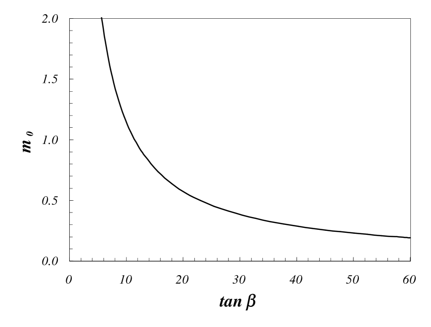
FIG. 4.: Allowed lower bounds for the common mass, $m_{o}$ (in eV), for varying $\tan\beta$, with $\Delta m_{atm}^{2}\approx 4\times 10^{-3}$ eV²,  $M_{N}=10^{13}$ GeV and $M_{S}=1$ TeV. For any other value of $M_{N}/M_{S}$, the corresponding lower value for $m_{o}$ scales accordingly.

- [1] S.M. Barr and I. Dorsner, hep-ph/0003058.
- [2] H. Fritzsch and Z. Xing, hep-ph/9903499; F. Vissani, hep-ph/9708483; Y. Koide and M. Fusaoka, hep-ph/9806516; G.K. Leontaris, S. Lola, C. Scheich and J.D. Vergados, Phys. Rev. D53, 6381 (1996); B.C. Allanach, hep-ph/9806294; V. Barger, S. Pakvasa, T.J. Weiler and K. Whisnant, Phys. Lett. B437, 107 (1998); A.J. Baltz, A.S. Goldhaber and M. Goldhaber, Phys. Rev. Lett. 81, 5730 (1998); R.N. Mohapatra and S. Nussinov, Phys. Lett. B441, 299 (1998); Y. Nomura and T. Yanagida, Phys. Rev. D59, 017303 (1999); S.K. Kang and C.S. Kim, Phys. Rev. D59, 091302 (1999); G. Altarelli and F. Feruglio, Phys. Lett. B439, 112 (1998) and JHEP 9811, 021 (1998); G. Altarelli, F. Feruglio and I. Masina, hep-ph/9907532; R. Barbieri, L.J. Hall, G. L. Kane and G.G. Ross, hep-ph/9901228; A.S. Joshipura and S. Rindani, Phys. Lett. B464, 239 (1999); E. Ma, Phys. Lett. B456, 201 (1999); R.N. Mohapatra, A. Perez-Lorenzana and C. Pires, Phys. Lett. B474, 355 (2000); Z. Berezhiani and A. Rossi, Phys. Lett. B367, 219 (1996); S.F. King, hep-ph/9904210; S.F. King and N.N. Singh, hep-ph/0006229.
- [3] K. S. Babu abd R. N. Mohapatra, Phys. Rev. Lett. 70, 2845 (1993); C. Albright and S. Barr, Phys. Rev. Lett. 85, 244 (2000); B. Brahmachari and R.N. Mohapatra, Phys. Rev. D58, 15003 (1998); K.S. Babu, J.C. Pati and F. Wilczek, hep-ph/9812538; K. T. Mahanthappa and M. Chen, hep-ph/0005292; T. Blazek, S. Raby and K. Tobe, Phys. Rev. D60, 113001 (1999); K. Oda, E. Takasugi, M. Tanaka and M. Yoshimura, Phys. Rev. D59, 055001 (1999).
- [4] K.R.S. Balaji, A.S. Dighe, R.N. Mohapatra and M.K. Parida, Phys. Rev. Lett. 84, 5034 (2000), hep-ph/0001310.
- [5] K.R.S. Balaji, A.S. Dighe, R.N. Mohapatra and M.K. Parida, Phys. Lett. B481, 33 (2000).
- [6] K.S. Babu, C.N. Leung and J. Pantaleone, Phys. Lett. B319, 191 (1993).
- [7] P.H. Chankowski and Z. Pluciennik, Phys. Lett. B316, 312 (1993).
- [8] B. Pendleton and G.G. Ross, Phys. Lett. B98, 291 (1981); C.T. Hill, Phys. Rev. D24, 691 (1981); M. Lanzagorta and G.G. Ross, Phys. Lett. B349, 319 (1995); E.A. Paschos, Z. Phys. C26, 235 (1984); S. Dimopoulous and S. Theodorakis, Phys. lett. B154, 153 (1985); S.A. Abel and B.C. Allanach, Phys. Lett. 415, 371 (1997).
- [9] Z. Maki, M. Nakagawa and S. Sakata, Prog. Theor. Phys. 28, 870 (1962).
- [10] P.H. Chankowski, W. Królikowski and S. Pokorski, hep-ph/9910231; J.A. Casas, J.R. Espinosa, A. Ibarra and I. Navaroo, hep-ph/9910420.
- [11] N. Haba, N. Okamura, M. Sugiura, hep-ph/9810471; N. Haba, Y. Matsui, N. Okamura, M. Sugiura, hep-ph/9908429; T. Miura, T. Shindou, E. Takasugi and M. Yoshimura, hep-ph/0005267; T. Miura et al., hep-ph/0007066; Zhi-zhong Xing, hep-ph/0011217.
- [12] J. Ellis and S. Lola, Phys. Lett. B458, 310, (1999); J. Ellis, G.K. Leontaris, S. Lola and D.V. Nanopoulos, Eur. Phys. J. C9, 389 (1999).
- [13] K. Scholderg, for SuperKamiokande Collaboration, hep-ph/9905016; T. Kajita, Invited talk at PASCOS 99, December 99.
- [14] Superkamiokande Collaboration Y. Fukuda et. al., Phys. Rev. Lett. 81, 1562 (1998); Kamiokande Collaboration S. Hatakiyama et. al., Phys. Rev. Lett. 81 2016 (1998).
- [15] D. White, for the LSND Collaboration, Nucl. Phys. Proc. Suppl. 77, 207 (1999).
- [16] CHOOZ Collaboration: M. Appollonio et. al. Phys. Lett. B420 397 (1998), hep-ex/9907037; PALOVERDE collaboration, talk by A. Piepke, Nu2000 conference.
- [17] H.V. Klapdor-Kleingrothaus et al., hep-ph/9910205.