Basics of QCD Perturbation Theory

Abstract

This is an introduction to the use of QCD perturbation theory, emphasizing generic features of the theory that enable one to separate short-time and long-time effects. I also cover some important classes of applications: electron-positron annihilation to hadrons, deeply inelastic scattering, and hard processes in hadron-hadron collisions.

Lectures at the TASI summer school, Boulder, Colorado, June 2000

1 Introduction

A prediction for experiment based on perturbative QCD combines a particular calculation of Feynman diagrams with the use of general features of the theory. The particular calculation is easy at leading order, not so easy at next-to-leading order and extremely difficult beyond the next-to-leading order. This calculation of Feynman diagrams would be a purely academic exercise if we did not use certain general features of the theory that allow the Feynman diagrams to be related to experiment: the renormalization group and the running coupling; the existence of infrared safe observables; the factorization property that allows us to isolate hadron structure in parton distribution functions.

In these lectures, I discuss these structural features of the theory that allow a comparison of theory and experiment. Along the way we will discover something about certain important processes: ${e^{+}e^{-}}$ annihilation; deeply inelastic scattering; hard processes in hadron-hadron collisions. By discussing the particular along with the general, I hope to arm the reader with information that speakers at research conferences take to be collective knowledge – knowledge that they assume the audience already knows.

Now here is the disclaimer. We will not learn how to do significant calculations in QCD perturbation theory. Three lectures is not enough for that.

I hope that the reader may be inspired to pursue the subjects discussed here in more detail. A good source is the Handbook of Perturbative QCD [1] by the CTEQ collaboration. More recently, Ellis, Stirling and Webber have written an excellent book [2] that covers the most of the subjects sketched in these lectures. For the reader wishing to gain a mastery of the theory, I can recommend the recent books on quantum field theory by Brown [3], Sterman [4], Peskin and Schroeder [5], and Weinberg [6]. Another good source, including both theory and phenomenology, is the lectures in the 1995 TASI proceedings, QCD and Beyond [7]. I have published a substantially similar set of lectures in the proceedings of the 1996 SLAC Summer school [8].

2 Electron-positron annihilation and jets

In this section, I explore the structure of the final state in QCD. I begin with the kinematics of $e^{+}e^{-}\to 3\ partons$, then examine the behavior of the cross section for $e^{+}e^{-}\to 3\ partons$ when two of the parton momenta become collinear or one parton momentum becomes soft. In order to illustrate better what is going on, I introduce a theoretical tool, null-plane coordinates. Using this tool, I sketch a space-time picture of the singularities that we find in momentum space. The singularities of perturbation theory correspond to long-time physics. We see that the structure of the final state suggested by this picture conforms well with what is actually observed.

I draw a the distinction between short-time physics, for which perturbation theory is useful, and long-time physics, for which the perturbative expansion is out of control. Finally, I discuss how certain experimental measurements can probe the short-time physics while avoiding sensitivity to the long-time physics.

2.1 Kinematics of $e^{+}e^{-}\to 3$ partons

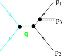
Figure 1: Feynman diagram for $e^{+}e^{-}\to q\,\bar{q}\,g$.

Consider the process $e^{+}e^{-}\to q\,\bar{q}\,g$, as illustrated in Fig. 1. Let $\sqrt{s}$ be the total energy in the c.m. frame and let $q^{\mu}$ be the virtual photon (or Z boson) momentum, so $q^{\mu}q_{\mu}=s$. Let $p_{i}^{\mu}$ be the momenta of the outgoing partons $(q,\bar{q},g)$ and let $E_{i}=p_{i}^{0}$ be the energies of the outgoing partons. It is useful to define energy fractions $x_{i}$ by

$${x_{i}={E_{i}\over\sqrt{s}/2}}={2p_{i}\cdot q\over s}.$$ (1)

Then

$${0<x_{i}}.$$ (2)

Energy conservation gives

$${\sum_{i}x_{i}}={2(\sum p_{i})\cdot q\over s}{=2}.$$ (3)

Thus only two of the $x_{i}$ are independent.

Let $\theta_{ij}$ be the angle between the momenta of partons $i$ and $j$. We can relate these angles to the momentum fractions as follows:

$$2p_{1}\cdot p_{2}=(p_{1}+p_{2})^{2}=(q-p_{3})^{2}=s-2q\cdot p_{3},$$ (4)

$$2E_{1}E_{2}(1-\cos\theta_{12})=s(1-x_{3}).$$ (5)

Dividing this equation by $s/2$ and repeating the argument for the two other pairs of partons, we obtain three relations for the angles $\theta_{ij}$:

$${x_{1}x_{2}(1-\cos\theta_{12})} = {2(1-x_{3})},$$

$${x_{2}x_{3}(1-\cos\theta_{23})} = {2(1-x_{1})},$$

$${x_{3}x_{1}(1-\cos\theta_{31})} = {2(1-x_{2})}.$$ (6)

We learn two things immediately. First,

$${x_{i}<1}.$$ (7)

Second, the three possible collinear configurations of the partons are mapped into $x_{i}$ space very simply:

$${\theta_{12}\to 0} \Leftrightarrow {x_{3}\to 1},$$

$${\theta_{23}\to 0} \Leftrightarrow {x_{1}\to 1},$$

$${\theta_{31}\to 0} \Leftrightarrow {x_{2}\to 1}.$$ (8)

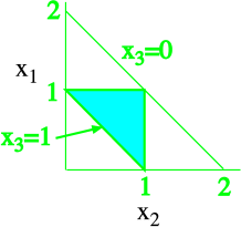
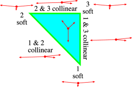
Figure 2: Allowed region for $(x_{1},x_{2})$. Then $x_{3}$ is $2-x_{1}-x_{2}$. The labels and small pictures in the right hand diagram show the physical configuration of the three partons corresponding to subregions in the allowed triangle.

The relations $0\leq x_{i}\leq 1$, together with $x_{3}=2-x_{1}-x_{2}$, imply that the allowed region for $(x_{1},x_{2})$ is a triangle, as shown in Fig. 2. The edges $x_{i}=1$ of the allowed region correspond to two partons being collinear, as also shown in Fig. 2. The corners $x_{i}=0$ correspond to one parton momentum being soft ($p_{i}^{\mu}\to 0$).

2.2 Structure of the cross section

One can easily calculate the cross section corresponding to Fig. 1 and the similar amplitude in which the gluon attaches to the antiquark line. The result is

$${1\over\sigma_{0}}\,{d\sigma\over dx_{1}dx_{2}}={\alpha_{s}\over 2\pi}C_{F}{x_{1}^{2}+x_{2}^{2}\over{(1-x_{1})(1-x_{2})}},$$ (9)

where $C_{F}=4/3$ and $\sigma_{0}=(4\pi\alpha^{2}/s)\sum Q_{f}^{2}$ is the total cross section for $e^{+}e^{-}\to hadrons$ at order $\alpha_{s}^{0}$. The cross section has collinear singularities:

$$(1-x_{1}) \to 0\,,\hskip 28.45274pt{\rm(2\&3\ collinear)};$$

$$(1-x_{2}) \to 0\,,\hskip 28.45274pt{\rm(1\&3\ collinear)}.$$ (10)

There is also a singularity when the gluon is soft: $x_{3}\to 0$. In terms of $x_{1}$ and $x_{2}$, this singularity occurs when

$$(1-x_{1})\to 0,\quad(1-x_{2})\to 0,\quad{(1-x_{1})\over(1-x_{2})}\sim const.$$ (11)

Let us write the cross section in a way that displays the collinear singularity at $\theta_{31}\to 0$ and the soft singularity at $E_{3}\to 0$:

$${1\over\sigma_{0}}{d\sigma\over dE_{3}\,d\cos\theta_{31}}={\alpha_{s}\over 2\pi}\,C_{F}\,{{f(E_{3},\theta_{31})}\over{E_{3}(1-\cos\theta_{31})}}.$$ (12)

Here ${f(E_{3},\theta_{31})}$ a rather complicated function. The only thing that we need to know about it is that it is finite for $E_{3}\to 0$ and for $\theta_{31}\to 0$.

Now look at the collinear singularity, ${\theta_{31}\to 0}$. If we integrate over the singular region holding $E_{3}$ fixed we find that the integral is divergent:

$$\int_{a}^{1}d\cos\theta_{31}\ {d\sigma\over dE_{3}\,d\cos\theta_{31}}=\log(\infty).$$ (13)

Similarly, if we integrate over the region of the soft singularity, holding $\theta_{31}$ fixed, we find that the integral is divergent:

$$\int_{0}^{a}dE_{3}\ {d\sigma\over dE_{3}\,d\cos\theta_{31}}=\log(\infty).$$ (14)

Evidently, perturbation theory is telling us that we should not take the perturbative cross section too literally. The total cross section for $e^{+}e^{-}\to hadrons$ is certainly finite, so this partial cross section cannot be infinite. What we are seeing is a breakdown of perturbation theory in the soft and collinear regions, and we should understand why.

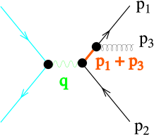
Figure 3: Cross section for $e^{+}e^{-}\to q\,\bar{q}\,g$, illustrating the singularity when the gluon is soft or collinear with the quark.

Where do the singularities come from? Look at Fig. 3 (in a physical gauge). The scattering matrix element ${\cal M}$ contains a factor $1/{(p_{1}+p_{3})}^{2}$ where

$$(p_{1}+p_{3})^{2}=2p_{1}\cdot p_{3}=2E_{1}E_{3}(1-\cos\theta_{31}).$$ (15)

Evidently, $1/{(p_{1}+p_{3})}^{2}$ is singular when $\theta_{31}\to 0$ and when $E_{3}\to 0$. The collinear singularity is somewhat softened because the numerator of the Feynman diagram contains a factor proportional to $\theta_{31}$ in the collinear limit. (This is not exactly obvious, but is easily seen by calculating. If you like symmetry arguments, you can derive this factor from quark helicity conservation and overall angular momentum conservation.) We thus find that

$$|{\cal M}|^{2}\propto\left[{\theta_{31}\over E_{3}\theta_{31}^{2}}\right]^{2}$$ (16)

for $E_{3}\to 0$ and $\theta_{31}\to 0$. Note the universal nature of these factors.

Integration over the double singular region of the momentum space for the gluon has the form

$$\int{E_{3}^{2}dE_{3}d\cos\theta_{31}d\phi\over E_{3}}\sim\int E_{3}dE_{3}d\theta_{31}^{2}d\phi.$$ (17)

Combining the integration with the matrix element squared gives

$$d\sigma\sim\int E_{3}dE_{3}d\theta_{31}^{2}d\phi\left[{\theta_{31}\over E_{3}\theta_{31}^{2}}\right]^{2}\sim\int{{dE_{3}}\over{E_{3}}}\ {{d\theta_{31}^{2}}\over{\theta_{31}^{2}}}\ d\phi.$$ (18)

Thus we have a double logarithmic divergence in perturbation theory for the soft and collinear region. With just a little enhancement of the argument, we see that there is a collinear divergence from integration over $\theta_{31}$ at finite $E_{3}$ and a separate soft divergence from integration over $E_{3}$ at finite $\theta_{31}$. Essentially the same argument applies to more complicated graphs. There are divergences when two final state partons become collinear and when a final state gluon becomes soft. Generalizing further [9], there are also divergences when several final state partons become collinear to one another or when several (with no net flavor quantum numbers) become soft.

We have seen that if we integrate over the singular region in momentum space with no cutoff, we get infinity. The integrals are logarithmically divergent, so if we integrate with an infrared cutoff $M_{IR}$, we will get big logarithms of $M_{IR}^{2}/s$. Thus the collinear and soft singularities represent perturbation theory out of control. Carrying on to higher orders of perturbation theory, one gets

$$1+\alpha_{s}\times({{\rm big}})+\alpha_{s}^{2}\times({{\rm big}})^{2}+\cdots.$$ (19)

If this expansion is in powers of $\alpha_{s}(M_{Z})$, we have $\alpha_{s}\ll 1$. Nevertheless, the big logarithms seem to spoil any chance of the low order terms of perturbation theory being a good approximation to any cross section of interest. Is the situation hopeless? We shall have to investigate further to see.

2.3 Interlude: Null plane coordinates

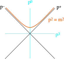
Figure 4: Null plane axes in momentum space.

In order to understand better the issue of singularities, it is helpful to introduce a concept that is generally quite useful in high energy quantum field theory, null plane coordinates. The idea is to describe the momentum of a particle using momentum components $p^{\mu}=(p^{+},p^{-},p^{1},p^{2})$ where

$${p^{\pm}=(p^{0}\pm p^{3})/\sqrt{2}}.$$ (20)

For a particle with large momentum in the $+z$ direction and limited transverse momentum, $p^{+}$ is large and $p^{-}$ is small. Often one chooses the plus axis so that a particle or group of particles of interest have large $p^{+}$ and small $p^{-}$ and $p_{T}$.

Using null plane components, the covariant square of $p^{\mu}$ is

$$p^{2}=2p^{+}p^{-}-{\bf p}_{T}^{2}.$$ (21)

Thus, for a particle on its mass shell, $p^{-}$ is

$$p^{-}={{\bf p}_{T}^{2}+m^{2}\over 2p^{+}}.$$ (22)

Note also that, for a particle on its mass shell,

$$p^{+}>0\,,\hskip 28.45274ptp^{-}>0\,.$$ (23)

Integration over the mass shell is

$$(2\pi)^{-3}\int{d^{3}\vec{p}\over 2\sqrt{\vec{p}^{2}+m^{2}}}\cdots=(2\pi)^{-3}\int\!d^{2}{\bf p}_{T}\,\int_{0}^{\infty}\!{dp^{+}\over 2p^{+}}\cdots.$$ (24)

We also use the plus/minus components to describe a space-time point $x^{\mu}$: $x^{\pm}=(x^{0}\pm$ $x^{3})/\sqrt{2}$. In describing a system of particles moving with large momentum in the plus direction, we are invited to think of $x^{+}$ as “time.” Classically, the particles in our system follow paths nearly parallel to the $x^{+}$ axis, evolving slowly as it moves from one $x^{+}=const.$ plane to another.

We relate momentum space to position space for a quantum system by Fourier transforming. In doing so, we have a factor $\exp(ip\cdot x)$, which has the form

$${p\cdot x=p^{+}x^{-}+p^{-}x^{+}-{\bf p}_{T}\cdot{\bf x}_{T}}.$$ (25)

Thus $x^{-}$ is conjugate to $p^{+}$ and $x^{+}$ is conjugate to $p^{-}$. That is a little confusing, but it is simple enough.

2.4 Space-time picture of the singularities

                 

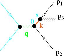
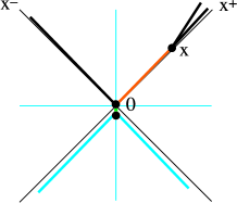
Figure 5: Correspondence between singularities in momentum space and the development of the system in space-time.

We now return to the singularity structure of $e^{+}e^{-}\to q\bar{q}g$. Define $p_{1}^{\mu}+p_{3}^{\mu}=k^{\mu}$. Choose null plane coordinates with $k^{+}$ large and ${\bf k}_{T}={\bf 0}$. Then $k^{2}=2k^{+}k^{-}$ becomes small when

$$k^{-}={{\bf p}_{3,T}^{2}\over 2p_{1}^{+}}+{{\bf p}_{3,T}^{2}\over 2p_{3}^{+}}$$ (26)

becomes small. This happens when ${\bf p}_{3,T}$ becomes small with fixed $p_{1}^{+}$ and $p_{3}^{+}$, so that the gluon momentum is nearly collinear with the quark momentum. It also happens when ${\bf p}_{3,T}$ and $p_{3}^{+}$ both become small with $p_{3}^{+}\propto|{\bf p}_{3,T}|$, so that the gluon momentum is soft. ( It also happens when the quark becomes soft, but there is a numerator factor that cancels the soft quark singularity.) Thus the singularities for a soft or collinear gluon correspond to small $k^{-}$.

Now consider the Fourier transform to coordinate space. The quark propagator in Fig. 5 is

$$S_{F}(k)=\int dx^{+}dx^{-}d{\bf x}\,\exp(i[k^{+}{x^{-}}+k^{-}{x^{+}}-{\bf k}\cdot{{\bf x}}])\ S_{F}(x).$$ (27)

When $k^{+}$ is large and $k^{-}$ is small, the contributing values of $x$ have small ${x^{-}}$ and large ${x^{+}}$. Thus the propagation of the virtual quark can be pictured in space-time as in Fig. 5. The quark propagates a long distance in the $x^{+}$ direction before decaying into a quark-gluon pair. That is, the singularities that can lead to divergent perturbative cross sections arise from interactions that happen a long time after the creation of the initial quark-antiquark pair.

2.5 Nature of the long-time physics

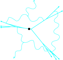
Figure 6: Typical paths of partons in space contributing to $e^{+}e^{-}\to hadrons$, as suggested by the singularities of perturbative diagrams. Short wavelength fields are represented by classical paths of particles. Long wavelength fields are represented by wavy lines.

Imagine dividing the contributions to a scattering cross section into long-time contributions and short-time contributions. In the long-time contributions, perturbation theory is out of control, as indicated in Eq. (19). Nevertheless the generic structure of the long-time contribution is of great interest. This structure is illustrated in Fig. 6. Perturbative diagrams have big contributions from space-time histories in which partons move in collinear groups and additional partons are soft and communicate over large distances, while carrying small momentum.

The picture of Fig. 6 is suggested by the singularity structure of diagrams at any fixed order of perturbation theory. Of course, there could be nonperturbative effects that would invalidate the picture. Since nonperturbative effects can be invisible in perturbation theory, one cannot claim that the structure of the final state indicated in Fig. 6 is known to be a consequence of QCD. One can point, however, to some cases in which one can go beyond fixed order perturbation theory and sum the most important effects of diagrams of all orders (for example, Ref. [10]). In such cases, the general picture suggested by Fig. 6 remains intact.

We thus find that perturbative QCD suggests a certain structure of the final state produced in $e^{+}e^{-}\to hadrons$: the final state should consist of jets of nearly collinear particles plus soft particles moving in random directions. In fact, this qualitative prediction is a qualitative success.

Given some degree of qualitative success, we may be bolder and ask whether perturbative QCD permits quantitative predictions. If we want quantitative predictions, we will somehow have to find things to measure that are not sensitive to interactions that happen long after the basic hard interaction. This is the subject of the next section.

2.6 The long-time problem

We have seen that perturbation theory is not effective for long-time physics. But the detector is a long distance away from the interaction, so it would seem that long-time physics has to be present.

Fortunately, there are some measurements that are not sensitive to long-time physics. An example is the total cross section to produce hadrons in $e^{+}e^{-}$ annihilation. Here effects from times $\Delta t\gg 1/\sqrt{s}$ cancel because of unitarity. To see why, note that the quark state is created from the vacuum by a current operator $J$ at some time $t$; it then develops from time $t$ to time $\infty$ according to the interaction picture evolution operator $U(\infty,t)$, when it becomes the final state $|N\rangle$. The cross section is proportional to the sum over $N$ of this amplitude times a similar complex conjugate amplitude with $t$ replaced by a different time $t^{\prime}$. We Fourier transform this with $\exp(-i\sqrt{s}\,(t-t^{\prime}))$, so that we can take $\Delta t\equiv t-t^{\prime}$ to be of order $1/\sqrt{s}$. Now replacing $\sum|N\rangle\langle N|$ by the unit operator and using the unitarity of the evolution operators $U$, we obtain

$$\sum_{N}\langle 0|J(t^{\prime})U(t^{\prime},\infty)|N\rangle\langle N|U(\infty,t)J(t)|0\rangle$$

$$=\langle 0|J(t^{\prime})U(t^{\prime},\infty)U(\infty,t)J(t)|0\rangle=\langle 0|J(t^{\prime})U(t^{\prime},t)J(t)|0\rangle.$$

Because of unitarity, the long-time evolution has canceled out of the cross section, and we have only evolution from $t$ to $t^{\prime}$.

There are three ways to view this result. First, we have the formal argument given above. Second, we have the intuitive understanding that after the initial quarks and gluons are created in a time $\Delta t$ of order $1/\sqrt{s}$, something will happen with probability 1. Exactly what happens is long-time physics, but we don’t care about it since we sum over all the possibilities $|N\rangle$. Third, we can calculate at some finite order of perturbation theory. Then we see infrared infinities at various stages of the calculations, but we find that the infinities cancel between real gluon emission graphs and virtual gluon graphs. An example is shown in Fig. 7.

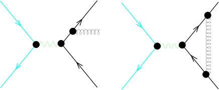
Figure 7: Cancellation between real and virtual gluon graphs. If we integrate the real gluon graph on the left times the complex conjugate of the similar graph with the gluon attached to the antiquark, we will get an infrared infinity. However the virtual gluon graph on the right times the complex conjugate of the Born graph is also divergent, as is the Born graph times the complex conjugate of the virtual gluon graph. Adding everything together, the infrared infinities cancel.

We see that the total cross section is free of sensitivity to long-time physics. If the total cross section were all you could look at, QCD physics would be a little boring. Fortunately, there are other quantities that are not sensitive to infrared effects. They are called infrared safe quantities.

To formulate the concept of infrared safety, consider a measured quantity that is constructed from the cross sections,

$${d\sigma[n]\over d\Omega_{2}dE_{3}d\Omega_{3}\cdots dE_{n}d\Omega_{n}},$$ (29)

to make $n$ hadrons in $e^{+}e^{-}$ annihilation. Here $E_{j}$ is the energy of the $j$th hadron and $\Omega_{j}=(\theta_{j},\phi_{j})$ describes its direction. We treat the hadrons as effectively massless and do not distinguish the hadron flavors. Following the notation of Ref. [11], let us specify functions ${\cal S}_{n}$ that describe the measurement we want, so that the measured quantity is

$${\cal I} = {1\over 2!}\int d\Omega_{2}\ {d\sigma[2]\over d\Omega_{2}}\ {{\cal S}_{2}}(p_{1}^{\mu},p_{2}^{\mu})$$ (30)

$$+{1\over 3!}\int d\Omega_{2}dE_{3}d\Omega_{3}\ {d\sigma[3]\over d\Omega_{2}dE_{3}d\Omega_{3}}\ {{\cal S}_{3}}(p_{1}^{\mu},p_{2}^{\mu},p_{3}^{\mu})$$

$$+{1\over 4!}\int d\Omega_{2}dE_{3}d\Omega_{3}dE_{4}d\Omega_{4}\$$

$$\hskip 56.9055pt\times{d\sigma[4]\over d\Omega_{2}dE_{3}d\Omega_{3}dE_{4}d\Omega_{4}}\ {{\cal S}_{4}}(p_{1}^{\mu},p_{2}^{\mu},p_{3}^{\mu},p_{4}^{\mu})$$

$$+\cdots.$$

The functions $\cal S$ are symmetric functions of their arguments. In order for our measurement to be infrared safe, we need

$${\cal S}_{n+1}(p_{1}^{\mu},\dots,{(1-\lambda)}{p_{n}^{\mu}},{\lambda}{p_{n}^{\mu}})={\cal S}_{n}(p_{1}^{\mu},\dots,{p_{n}^{\mu}})$$ (31)

for $0\leq{\lambda}\leq 1$.

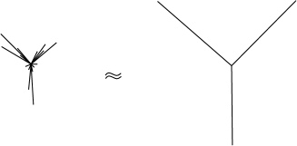
Figure 8: Infrared safety. In an infrared safe measurement, the three jet event shown on the left should be (approximately) equivalent to an ideal three jet event shown on the right.

What does this mean? The physical meaning is that the functions ${\cal S}_{n}$ and ${\cal S}_{n-1}$ are related in such a way that the cross section is not sensitive to whether or not a mother particle divides into two collinear daughter particles that share its momentum. The cross section is also not sensitive to whether or not a mother particle decays to a daughter particle carrying all of its momentum and a soft daughter particle carrying no momentum. The cross section is also not sensitive to whether or not two collinear particles combine, or a soft particle is absorbed by a fast particle. All of these decay and recombination processes can happen with large probability in the final state long after the hard interaction. But, by construction, they don’t matter as long as the sum of the probabilities for something to happen or not to happen is one.

Another version of the physical meaning is that for an IR-safe quantity a physical event with hadron jets should give approximately the same measurement as a parton event with each jet replaced by a parton, as illustrated in Fig. 8. To see this, we simply have to delete soft particles and combine collinear particles until three jets have become three particles.

In a calculation of the measured quantity $\cal I$, we simply calculate with partons instead of hadrons in the final state. The calculational meaning of the infrared safety condition is that the infrared infinities cancel. The argument is that the infinities arise from soft and collinear configurations of the partons, that these configurations involve long times, and that the time evolution operator is unitary.

I have started with an abstract formulation of infrared safety. It would be good to have a few examples. The easiest is the total cross section, for which

$${\cal S}_{n}(p_{1}^{\mu},\dots,p_{n}^{\mu})=1.$$ (32)

A less trivial example is the thrust distribution. One defines the thrust ${\cal T}_{n}$ of an $n$ particle event as

$${\cal T}_{n}(p_{1}^{\mu},\dots,p_{n}^{\mu})=\max_{\vec{u}}{\sum_{i=1}^{n}|\vec{p}_{i}\cdot\vec{u}|\over\sum_{i=1}^{n}|\vec{p}_{i}|}\ .$$ (33)

Here $\vec{u}$ is a unit vector, which we vary to maximize the sum of the absolute values of the projections of $\vec{p}_{i}$ on $\vec{u}$. Then the thrust distribution $(1/\sigma_{tot})\,d\sigma/dT$ is defined by taking

$${\cal S}_{n}(p_{1}^{\mu},\dots,p_{n}^{\mu})=(1/\sigma_{tot})\ \delta\!\left(T-{\cal T}_{n}(p_{1}^{\mu},\dots,p_{n}^{\mu})\right)\ .$$ (34)

It is a simple exercise to show that the thrust of an event is not affected by collinear parton splitting or by zero momentum partons. Therefore the thrust distribution is infrared safe.

Another example is the energy-energy correlation function $d\Sigma/d\cos(\theta)$ [12]:

$${\cal S}_{n}(p_{1}^{\mu},\dots,p_{n}^{\mu})=\sum_{ij}{E_{i}E_{j}\over s}\ \delta\left(\cos(\theta_{ij})-\cos(\theta)\right)\ .$$ (35)

This measures the correlation between the energies measured by detectors separated by an angle $\theta$ as depicted in Fig. 9. Is this infrared safe? Note that the contribution from a particle with $E_{i}\to 0$ drops out. In addition, replacing one particle by two collinear particles doesn’t change the thrust:

$$(1-\lambda)\,E_{n}\,E_{j}+\lambda\,E_{n}\,E_{j}=E_{n}\,E_{j}.$$ (36)

This works for the autocorrelation term too:

$$(1-\lambda)^{2}\,E_{n}^{2}+2\lambda(1-\lambda)\,E_{n}^{2}+\lambda^{2}\,E_{n}^{2}=E_{n}^{2}.$$ (37)

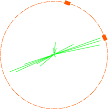
Figure 9: The energy-energy correlation function

A final example is the cross section to make $n$ jets, $\sigma_{n}$. Intuitively, a jet is supposed to be a spray of particles all going in approximately the same direction. To make this precise, we need a definite algorithm. There are several algorithms to choose from. Here is the simplest (but not the best) one.

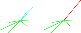
Figure 10: Jet definition

Start with a list of momenta $p_{1}^{\mu},p_{2}^{\mu},\dots,p_{N}^{\mu}$. At the start, these represent the momenta of particles. (In a perturbative calculation, they are the momenta of partons.) Choose a parameter $y_{\rm cut}$. Now proceed through the following steps:

1. Find the pair $(i,j)$ such that $(p_{i}+p_{j})^{2}$ is the smallest.

2. If $(p_{i}+p_{j})^{2}>y_{\rm cut}\,s$, exit. Else continue.

3. Replace the two momenta $p_{i}$ and $p_{j}$ in the list by their sum $p_{k}^{\mu}=p_{i}^{\mu}+p_{j}^{\mu}$.

4. Go to 1.

This produces a list of momenta $p_{i}$ of jets. $\sigma_{n}$ is the cross section to have $n$ jets. The infrared safety of $\sigma_{n}$ is easy to prove given our experience with the previous examples.

There are several variations on this theme. For instance, change the resolution condition or the combination prescription. A comparison of methods can be found in Ref. [13]. I discuss jet cross sections for hadron collisions in Sec. 5.4.

Before leaving this subject, I should mention another way to eliminate sensitivity to long-time physics. Consider the cross section

$${d\sigma(e^{+}e^{-}\to\pi+X)\over dE_{\pi}}.$$ (38)

This cross section can be written as a convolution of two factors. The first factor is a calculated “hard scattering cross section” for $e^{+}e^{-}\to{quark}+X$ or $e^{+}e^{-}\to{gluon}+X$. The second factor is a “parton decay function” for ${quark}\to\pi+X$ or ${gluon}\to\pi+X$. These functions contain the long-time sensitivity and are to be measured, since they cannot be calculated perturbatively. However, once they are measured in one process, they can be used for another process. This final state factorization is similar to the initial state factorization involving parton distribution functions, which we will discuss later. (See Refs. [1],[2],[14] for more information.)

3 The smallest time scales

In this section, I explore the physics of time scales smaller than $1/\sqrt{s}$. One way of looking at this physics is to say that it is plagued by infinities and we can manage to hide the infinities. A better view is that the short-time physics contains wonderful truths that we would like to discover – truths about grand unified theories, quantum gravity and the like. However, quantum field theory is arranged so as to effectively hide the truth from our experimental apparatus, which can probe with a time resolution of only an inverse half TeV.

I first outline what renormalization does to hide the ugly infinities or the beautiful truth. Then I describe how renormalization leads to the running coupling. Because of renormalization, calculated quantities depend on a renormalization scale. I look at how this dependence works and how the scale can be chosen. Finally, I discuss how one can use experiment to look for the hidden physics beyond the Standard Model, taking high $E_{T}$ jet production in hadron collisions as an example.

3.1 What renormalization does

In any Feynman graph, one can insert perturbative corrections to the vertices and the propagation of particles, as illustrated in Fig. 11. The loop integrals in these graphs will get big contributions from momenta much larger than $\sqrt{s}$. That is, there are big contributions from interactions that happen on time scales much smaller than $1/\sqrt{s}$. I have tried to illustrate this in the figure. The virtual vector boson propagates for a time $1/\sqrt{s}$, while the virtual fluctuations that correct the electroweak vertex and the quark propagator occur over a time $\Delta t$ that can be much smaller than $1/\sqrt{s}$.

Let us pick an ultraviolet cutoff $M$ that is much larger than $\sqrt{s}$, so that we calculate the effect of fluctuations with $1/M<\Delta t$ exactly, up to some order of perturbation theory. What, then, is the effect of virtual fluctuations on smaller time scales, $\Delta t$ with $\Delta t<1/M$ but, say, $\Delta t$ still larger than $t_{\rm Plank}$, where gravity takes over? Let us suppose that we are willing to neglect contributions to the cross section that are of order $\sqrt{s}/M$ or smaller compared to the cross section itself. Then there is a remarkable theorem [15]: the effects of the fluctuations are not particularly small, but they can be absorbed into changes in the couplings of the theory. (There are also changes in the masses of the theory and adjustments to the normalizations of the field operators, but we can concentrate on the effect on the couplings.)

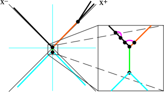
Figure 11: Renormalization. The effect of the very small time interactions pictured are absorbed into the running coupling.

The program of absorbing very short-time physics into a few parameters goes under the name of renormalization. There are several schemes available for renormalizing. Each of them involves the introduction of some scale parameter that is not intrinsic to the theory but tells how we did the renormalization. Let us agree to use  MS  renormalization (see Ref. [15] for details). Then we introduce an  MS  renormalization scale $\mu$. A good (but approximate) way of thinking of $\mu$ is that the physics of time scales $\Delta t\ll 1/\mu$ is removed from the perturbative calculation. The effect of the small time physics is accounted for by adjusting the value of the strong coupling, so that its value depends on the scale that we used: $\alpha_{s}=\alpha_{s}(\mu)$. (The value of the electromagnetic coupling also depends on $\mu$.)

3.2 The running coupling

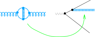
Figure 12: Short-time fluctuations in the propagation of the gluon field absorbed into the running strong coupling.

We account for time scales much smaller than $1/\mu$ by using the running coupling $\alpha_{s}(\mu)$. That is, a fluctuation such as that illustrated in Fig. 12 can be dropped from a calculation and absorbed into the running coupling that describes the probability for the quark in the figure to emit the gluon. The $\mu$ dependence of $\alpha_{s}(\mu)$ is given by a certain differential equation, called the renormalization group equation (see Ref. [15]):

$${d\over d\ln(\mu^{2})}\,{\alpha_{s}(\mu)\over\pi}=\beta(\alpha_{s}(\mu))=-\beta_{0}\,\left(\alpha_{s}(\mu)\over\pi\right)^{2}-\beta_{1}\,\left(\alpha_{s}(\mu)\over\pi\right)^{3}+\cdots.$$ (39)

One calculates the beta function $\beta(\alpha_{s})$ perturbatively in QCD. The first coefficient, with the conventions used here, is

$$\beta_{0}=(33-2\,N_{f})/12\,,$$ (40)

where $N_{f}$ is the number of quark flavors.

Of course, at time scales smaller than a very small cutoff $1/M$ (at the “GUT scale,” say) there is completely different physics operating. Therefore, if we use just QCD to adjust the strong coupling, we can say that we are accounting for the physics between times $1/M$ and $1/\mu$. The value of $\alpha_{s}$ at $\mu_{0}\approx M$ is then the boundary condition for the differential equation. See Fig. 13.

Figure 13: Time scales accounted for by explicit fixed order perturbative calculation and by use of the renormalization group.

The renormalization group equation sums the effects of short-time fluctuations of the fields. To see what one means by “sums” here, consider the result of solving the renormalization group equation with all of the $\beta_{i}$ beyond $\beta_{0}$ set to zero:

$$\alpha_{s}(\mu) \approx \alpha_{s}(M)-(\beta_{0}/\pi)\ln(\mu^{2}/M^{2})\ \alpha_{s}^{2}(M)$$ (41)

$$\quad+(\beta_{0}/\pi)^{2}\ln^{2}(\mu^{2}/M^{2})\ \alpha_{s}^{3}(M)+\cdots$$

$$= {\alpha_{s}(M)\over 1+(\beta_{0}/\pi)\,\alpha_{s}(M)\ln(\mu^{2}/M^{2})}.$$

A series in powers of $\alpha_{s}(M)$ – that is the strong coupling at the GUT scale – is summed into a simple function of $\mu$. Here $\alpha_{s}(M)$ appears as a parameter in the solution.

Note a crucial and wonderful fact. The value of $\alpha_{s}(\mu)$ decreases as $\mu$ increases. This is called “asymptotic freedom.” Asymptotic freedom implies that QCD acts like a weakly interacting theory on short time scales. It is true that quarks and gluons are strongly bound inside nucleons, but this strong binding is the result of weak forces acting collectively over a long time.

In Eq. (41), we are invited to think of the graph of $\alpha_{s}(\mu)$ versus $\mu$. The differential equation that determines this graph is characteristic of QCD. There could, however, be different versions of QCD with the same differential equation but different curves, corresponding to different boundary values $\alpha_{s}(M)$. Thus the parameter $\alpha_{s}(M)$ tells us which version of QCD we have. To determine this parameter, we consult experiment. Actually, Eq. (41) is not the most convenient way to write the solution for the running coupling. A better expression is

$$\alpha_{s}(\mu)\approx{\pi\over\beta_{0}\ln(\mu^{2}/\Lambda^{2})}.$$ (42)

Here we have replaced $\alpha_{s}(M)$ by a different (but completely equivalent) parameter $\Lambda$. A third form of the running coupling is

$$\alpha_{s}(\mu)\approx{\alpha_{s}(M_{Z})\over 1+(\beta_{0}/\pi)\,\alpha_{s}(M_{Z})\ln(\mu^{2}/M_{Z}^{2})}.$$ (43)

Here the value of $\alpha_{s}(\mu)$ at $\mu=M_{Z}$ labels the version of QCD that obtains in our world.

In any of the three forms of the running coupling, one should revise the equations to account for the second term in the beta function in order to be numerically precise.

3.3 The choice of scale

In this section, we consider the choice of the renormalization scale $\mu$ in a calculated cross section. Consider, as an example, the cross section for $e^{+}e^{-}\to{\rm hadrons}$ via virtual photon decay. Let us write this cross section in the form

$$\sigma_{\rm tot}={4\pi\alpha^{2}\over s}\left(\sum_{f}Q_{f}^{2}\right)\left[1+\Delta\right].$$ (44)

Here $s$ is the square of the c.m. energy, $\alpha$ is $e^{2}/(4\pi)$, and $Q_{f}$ is the electric charge in units of $e$ carried by the quark of flavor $f$, with $f=u,d,s,c,b$. The nontrivial part of the calculated cross section is the quantity $\Delta$, which contains the effects of the strong interactions. Using  MS  renormalization with scale $\mu$, one finds (after a lot of work) that $\Delta$ is given by Ref. [16]:

$$\Delta={\alpha_{s}({\mu})\over\pi}+\left[1.4092+1.9167\ \ln\left({\mu^{2}}/s\right)\right]\left({\alpha_{s}({\mu})\over\pi}\right)^{\!2}$$

$$\quad+\left[-12.805+7.8186\ \ln\left({\mu^{2}}/s\right)+3.674\ \ln^{2}\!\left({\mu^{2}}/s\right)\right]\left({\alpha_{s}({\mu})\over\pi}\right)^{\!3}$$

$$\quad+\cdots.$$ (45)

Here, of course, one should use for $\alpha_{s}(\mu)$ the solution of the renormalization group equation (39) with at least two terms included.

As discussed in the preceding subsection, when we renormalize with scale $\mu$, we are defining what we mean by the strong coupling. Thus $\alpha_{s}$ in Eq. (45) depends on $\mu$. The perturbative coefficients in Eq. (45) also depend on $\mu$. On the other hand, the physical cross section does not depend on $\mu$:

$${d\over d\ln\mu^{2}}\,\Delta=0.$$ (46)

That is because $\mu$ is just an artifact of how we organize perturbation theory, not a parameter of the underlying theory.

Let us consider Eq. (46) in more detail. Write $\Delta$ in the form

$$\Delta\sim\sum_{n=1}^{\infty}c_{n}(\mu)\ \alpha_{s}(\mu)^{n}.$$ (47)

If we differentiate not the complete infinite sum but just the first $N$ terms, we get minus the derivative of the sum from $N+1$ to infinity. This remainder is of order $\alpha_{s}^{N+1}$ as $\alpha_{s}\to 0$. Thus

$${d\over d\ln\mu^{2}}\sum_{n=1}^{N}c_{n}(\mu)\ \alpha_{s}(\mu)^{n}\sim{\cal O}(\alpha_{s}(\mu)^{N+1}).$$ (48)

That is, the harder we work calculating more terms, the less the calculated cross section depends on $\mu$.

Since we have not worked infinitely hard, the calculated cross section depends on $\mu$. What choice shall we make for $\mu$? Clearly, $\ln\left(\mu^{2}/s\right)$ should not be big. Otherwise the coefficients $c_{n}(\mu)$ are large and the “convergence” of perturbation theory will be spoiled. There are some who will argue that one scheme or the other for choosing $\mu$ is the “best.” You are welcome to follow whichever advisor you want. I will show you below that for a well behaved quantity like $\Delta$ the precise choice makes little difference, as long as you obey the common sense prescription that $\ln\left(\mu^{2}/s\right)$ not be big.

3.4 An example

                              $\Delta(\mu)$

         $\ln_{2}(\mu/\sqrt{s})$

Figure 14: Dependence of $\Delta(\mu)$ on the  MS  renormalization scale $\mu$. The falling curve is $\Delta_{1}$. The flatter curve is $\Delta_{2}$. The horizontal lines indicates the amount of variation of $\Delta_{2}$ when $\mu$ varies by a factor 2.

Let us consider a quantitative example of how $\Delta(\mu)$ depends on $\mu$. This will also give us a chance to think about the theoretical error caused by replacing $\Delta$ by the sum $\Delta_{n}$ of the first $n$ terms in its perturbative expansion. Of course, we do not know what this error is. All we can do is provide an estimate. (Our discussion will be rather primitive. For a more detailed error estimate for the case of the hadronic width of the $Z$ boson, see Ref. [17].)

Let us think of the error estimate in the spirit of a “$1\,\sigma$” theoretical error: we would be surprised if $|\Delta_{n}-\Delta|$ were much less than the error estimate and we would also be surprised if this quantity were much more than the error estimate. Here, one should exercise a little caution. We have no reason to expect that theory errors are gaussian distributed. Thus a $4\,\sigma$ difference between $\Delta_{n}$ and $\Delta$ is not out of the question, while a $4\,\sigma$ fluctuation in a measured quantity with purely statistical, gaussian errors is out of the question.

Take $\alpha_{s}(M_{Z})=0.117$, $\sqrt{s}=34{\ \rm GeV}$, 5 flavors. In Fig. 14, I plot $\Delta(\mu)$ versus ${p}$ defined by

$$\mu=2^{p}\sqrt{s}.$$ (49)

The steeply falling curve is the order $\alpha_{s}^{1}$ approximation to $\Delta(\mu)$, $\Delta_{1}(\mu)={\alpha_{s}(\mu)/\pi}$. Notice that if we change $\mu$ by a factor 2, $\Delta_{1}(\mu)$ changes by about 0.006. If we had no other information than this, we might pick $\Delta_{1}(\sqrt{s})\approx 0.044$ as the “best” value and assign a $\pm 0.006$ error to this value. (There is no special magic to the use of a factor of 2 here. The reader can pick any factor that seems reasonable.)

Another error estimate can be based on the simple expectation that the coefficients of $\alpha_{s}^{n}$ are of order 1 for the first few terms. (Eventually, they will grow like $n!$. Ref. [17] takes this into account, but we ignore it here.) Then the first omitted term should be of order $\pm 1\times\alpha_{s}^{2}\approx\pm 0.020$ using $\alpha_{s}(34\ {\ \rm GeV})\approx 0.14$. Since this is bigger than the previous $\pm 0.006$ error estimate, we keep this larger estimate: $\Delta\approx 0.044\pm 0.020$.

Returning now to Fig. 14, the second curve is the order $\alpha_{s}^{2}$ approximation, $\Delta_{2}(\mu)$. Note that $\Delta_{2}(\mu)$ is less dependent on $\mu$ than $\Delta_{1}(\mu)$.

What value would we now take as our best estimate of $\Delta$? One idea is to choose the value of $\mu$ at which $\Delta_{2}(\mu)$ is least sensitive to $\mu$. This idea is called the principle of minimal sensitivity [18]:

$$\Delta_{PMS}=\Delta(\mu_{PMS})\,,\hskip 28.45274pt\left[{d\Delta(\mu)\over d\ln\mu}\right]_{\mu=\mu_{PMS}}=0.$$ (50)

This prescription gives $\Delta\approx 0.0470$. Note that this is about 0.003 away from our previous estimate, $\Delta\approx 0.0440$. Thus our previous error estimate of 0.020 was too big, and we should be surprised that the result changed so little. We can make a new error estimate by noting that $\Delta_{2}(\mu)$ varies by about 0.0012 when $\mu$ changes by a factor $2$ from $\mu_{PMS}$. Thus we might estimate that $\Delta\approx 0.0470$ with an error of $\pm 0.0012$. This estimate is represented by the two horizontal lines in Fig. 14.

An alternative error estimate can be based on the next term being of order $\pm 1\times\alpha_{s}^{3}(34\ GeV)\approx 0.003$. Since this is bigger than the previous $\pm 0.0012$ error estimate, we keep this larger estimate: $\Delta\approx 0.0470\pm 0.003$.

I should emphasize that there are other ways to pick the “best” value for $\Delta$. For instance, one can use the BLM method [19], which is based on choosing the $\mu$ that sets to zero the coefficient of the number of quark flavors in $\Delta_{2}(\mu)$. Since the graph of $\Delta_{2}(\mu)$ is quite flat, it makes very little difference which method one uses.

$\Delta(\mu)$                                                                $\Delta(\mu)$

                        $\log_{2}(\mu/\sqrt{s})$                                                            $\log_{2}(\mu/\sqrt{s})$

                 

Figure 15: Dependence of $\Delta(\mu)$ on the  MS  renormalization scale $\mu$, first with a normal scale and then with an expanded scale. The falling curve is $\Delta_{1}$. The flatter curve is $\Delta_{2}$. The still flatter curve is $\Delta_{3}$. The horizontal lines represent the variation of $\Delta_{2}$ when $\mu$ varies by a factor 2.

Now let us look at $\Delta(\mu)$ evaluated at order $\alpha_{s}^{3}$, $\Delta_{3}(\mu)$. Here we make use of the full formula in Eq. (45). In Fig. 15, I plot $\Delta_{3}(\mu)$ along with $\Delta_{2}(\mu)$ and $\Delta_{1}(\mu)$. The variation of $\Delta_{3}(\mu)$ with $\mu$ is smaller than that of $\Delta_{2}(\mu)$. The improvement is not overwhelming, but is apparent particularly at small $\mu$.

It is a little difficult to see what is happening in the first graph of Fig. 15, so I show the same thing with an expanded scale. (Here the error band based on the $\mu$ dependence of $\Delta_{2}$ is also indicated. Recall that we decided that this error band was an underestimate.) The curve for $\Delta_{3}(\mu)$ has zero derivative at two places. The corresponding values are $\Delta\approx 0.0436$ and $\Delta\approx 0.0456$. If I take the best value of $\Delta$ to be the average of these two values and the error to be half the difference, I get $\Delta\approx 0.0446\pm 0.0010$.

The alternative error estimate is $\pm 1\times\alpha_{s}^{4}(34\ {\ \rm GeV})\approx 0.0004$. We keep the larger error estimate of $\pm 0.0010$.

Was the previous error estimate valid? We guessed $\Delta\approx 0.0470\pm 0.003$. Our new best estimate is 0.0446. The difference is 0.0024, which is in line with our previous error estimate. Had we used the error estimate $\pm 0.0012$ based on the $\mu$ dependence, we would have underestimated the difference, although we would not have been too far off.

3.5 Beyond the Standard Model

We have seen how the renormalization group enables us to account for QCD physics at time scales much smaller than $\sqrt{s}$, as indicated in Fig. 13. However, at some scale $\Delta t\sim 1/M$, we run into the unknown!

How can we see the unknown in current experiments? First, the unknown physics affects $\alpha_{s}$, $\alpha_{em}$, $\sin^{2}(\theta_{W})$. Second, the unknown physics affects masses of $u,d,\dots,e,\mu,\dots$. That is, the unknown physics (presumably) determines the parameters of the Standard Model. These parameters have been well measured. Thus, a Nobel prize awaits the physicist who figures out how to use a model for the unknown physics to predict these parameters.

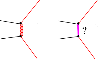
Figure 16: New physics at a TeV scale. In the first diagram, quarks scatter by gluon exchange. In the second diagram, the quarks exchange a new object with a TeV mass, or perhaps exchange some of the constituents out of which quarks are made.

There is another way that as yet unknown physics can affect current experiments. Suppose that quarks can scatter by the exchange of some new particle with a heavy mass $M$, as illustrated in Fig. 16, and suppose that this mass is not too enormous, only a few TeV. Perhaps the new particle isn’t a particle at all, but is a pair of constituents that live inside of quarks. As mentioned above, this physics affects the parameters of the Standard Model. However, unless we can predict the parameters of the Standard Model, this effect does not help us. There is, however, another possible clue. The physics at the TeV scale can introduce new terms into the lagrangian that we can investigate in current experiments.

In the second diagram in Fig. 16, the two vertices are never at a separation in time greater than $1/M$, so that our low energy probes cannot resolve the details of the structure. As long as we stick to low energy probes, $\sqrt{s}\ll M$, the effect of the new physics can be summarized by adding new terms to the lagrangian of QCD. A typical term might be

$${\Delta{\cal L}={\tilde{g}^{2}\over M^{2}}\ \bar{\psi}\gamma^{\mu}\psi\ \bar{\psi}\gamma_{\mu}\psi.}$$ (51)

There is a factor $\tilde{g}^{2}$ that represents how well the new physics couples to quarks. The most important factor is the factor $1/M^{2}$. This factor must be there: the product of field operators has dimension 6 and the lagrangian has dimension 4, so there must be a factor with dimension $-2$. Taking this argument one step further, the product of field operators in $\Delta{\cal L}$ must have a dimension greater than 4 because any product of field operators having dimension equal to or less than 4 that respects the symmetries of the Standard Model is already included in the lagrangian of the Standard Model.

3.6 Looking for new terms in the effective lagrangian

How can one detect the presence in the lagrangian of a term like that in Eq. (51)? These terms are small. Therefore we need either a high precision experiment, or an experiment that looks for some effect that is forbidden in the Standard Model, or an experiment that has moderate precision and operates at energies that are as high as possible.

Let us consider an example of the last of these possibilities, $p+\bar{p}\to jet+X$ as a function of the transverse energy ($\sim P_{T}$) of the jet. The new term in the lagrangian should add a little bit to the observed cross section that is not included in the standard QCD theory. When the transverse energy $E_{T}$ of the jet is small compared to $M$, we expect

$${{{\rm Data}-{\rm Theory}\over{\rm Theory}}}\propto\tilde{g}^{2}{{E_{T}^{2}}\over M^{2}}.$$ (52)

Here the factor $\tilde{g}^{2}/M^{2}$ follows because $\Delta{\cal L}$ contains this factor. The factor $E_{T}^{2}$ follows because the left hand side is dimensionless and $E_{T}$ is the only factor with dimension of mass that is available.

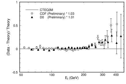
Figure 17: Jet cross sections from CDF and D0 compared to QCD theory. (Data $-$ Theory)/Theory is plotted versus the transverse energy $E_{T}$ of the jet. The theory here is next-to-leading order QCD using the CTEQ3M parton distribution. Source: Ref. [20]

In Fig. 17, I show a plot comparing experimental jet cross sections from CDF [21] and D0 [22] compared to next-to-leading order QCD theory. The theory works fine for $E_{T}<200{\ \rm GeV}$, but for $200{\ \rm GeV}<E_{T}$, there appears to be a systematic deviation of just the form anticipated in Eq. (52).

This example illustrates the idea of how small distance physics beyond the Standard Model can leave a trace in the form of small additional terms in the effective lagrangian that controls physics at currently available energies. However, in this case, there is some indication that the observed effect might be explained by some combination of the experimental systematic error and the uncertainties inherent in the theoretical prediction [23]. In particular, the prediction is sensitive to the distributions of quarks and gluons contained in the colliding protons, and the gluon distribution in the kinematic range of interest here is rather poorly known. In the next section, we turn to the definition, use, and measurement of the distributions of quarks and gluons in hadrons.

4 Deeply inelastic scattering

Until now, I have concentrated on hard scattering processes with leptons in the initial state. For such processes, we have seen that the hard part of the process can be described using perturbation theory because $\alpha_{s}(\mu)$ gets small as $\mu$ gets large. Furthermore, we have seen how to isolate the hard part of the interaction by choosing an infrared safe observable. But what about hard processes in which there are hadrons in the initial state? Since the fundamental hard interactions involve quarks and gluons, the theoretical description necessarily involves a description of how the quarks and gluons are distributed in a hadron. Unfortunately, the distribution of quarks and gluons in a hadron is controlled by long-time physics. We cannot calculate the relevant distribution functions perturbatively (although a calculation in lattice QCD might give them, in principle). Thus we must find how to separate the short-time physics from the parton distribution functions and we must learn how the parton distribution functions can be determined from the experimental measurements.

In this section, I discuss parton distribution functions and their role in deeply inelastic lepton scattering (DIS). This includes $e+p\to e+X$ and $\nu+p\to e+X$ where the momentum transfer from the lepton is large. I first outline the kinematics of deeply inelastic scattering and define the structure functions $F_{1}$, $F_{2}$ and $F_{3}$ used to describe the process. By examining the space-time structure of DIS, we will see how the cross section can be written as a convolution of two factors, one of which is the parton distribution functions and the other of which is a cross section for the lepton to scatter from a quark or gluon. This factorization involves a scale $\mu_{F}$ that, roughly speaking, divides the soft from the hard regime; I discuss the dependence of the calculated cross section on $\mu_{F}$. With this groundwork laid, I give the  MS  definition of parton distribution functions in terms of field operators and discuss the evolution equation for the parton distributions. I close the section with some comments on how the parton distributions are, in practice, determined from experiment.

4.1 Kinematics of deeply inelastic lepton scattering

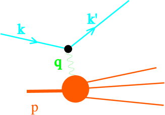
Figure 18: Kinematics of deeply inelastic scattering

In deeply inelastic scattering, a lepton with momentum $k^{\mu}$ scatters on a hadron with momentum $p^{\mu}$. In the final state, one observes the scattered lepton with momentum $k^{\prime\mu}$ as illustrated in Fig. 18. The momentum transfer

$$q^{\mu}=k^{\mu}-k^{\prime\mu}$$ (53)

is carried on a photon, or a $W$ or $Z$ boson.

The interaction between the vector boson and the hadron depends on the variables $q^{\mu}$ and $p^{\mu}$. From these two vectors we can build two scalars (not counting $m^{2}=p^{2}$). The first variable is

$${Q^{2}}=-q^{2},$$ (54)

where the minus sign is included so that $Q^{2}$ is positive. The second scalar is the dimensionless Bjorken variable,

$${x_{\rm bj}}={Q^{2}\over 2p\cdot q}.$$ (55)

(In the case of scattering from a nucleus containing $A$ nucleons, one replaces $p^{\mu}$ by $p^{\mu}/A$ and defines $x_{\rm bj}=A\,{Q^{2}/(2p\cdot q)}$.)

One calls the scattering deeply inelastic if $Q^{2}$ is large compared to $1\ {\ \rm GeV}^{2}$. Traditionally, one speaks of the scaling limit, $Q^{2}\to\infty$ with $x_{\rm bj}$ fixed. Actually, the asymptotic theory to be described below works pretty well if $Q^{2}$ is bigger than, say, $4\,{\ \rm GeV}^{2}$ and $x_{\rm bj}$ is anywhere in the experimentally accessible range, roughly $10^{-4}<x_{\rm bj}<0.5$.

The invariant mass squared of the hadronic final state is $W^{2}=(p+q)^{2}$. In the scaling regime of large $Q^{2}$ one has

$$W^{2}=m^{2}+{1-x_{\rm bj}\over x_{\rm bj}}\,Q^{2}\gg m^{2}.$$ (56)

This justifies saying that the scattering is not only inelastic but deeply inelastic.

We have spoken of the scalar variables that one can form from $p^{\mu}$ and $q^{\mu}$. Using the lepton momentum $k^{\mu}$, one can also form the dimensionless variable

$$y={p\cdot q\over p\cdot k}.$$ (57)

4.2 Structure functions for DIS

One can make quite a lot of progress in understanding the theory of deeply inelastic scattering without knowing anything about QCD except its symmetries. One expresses the cross section in terms of three structure functions, which are functions of $x_{\rm bj}$ and $Q^{2}$ only.

Suppose that the initial lepton is a neutrino, $\nu_{\mu}$, and the final lepton is a muon. Then in Fig. 18 the exchanged vector boson, call it $V$, is a $W$ boson, with mass $M_{V}=M_{W}$. Alternatively, suppose that both the initial and final leptons are electrons and let the exchanged vector boson be a photon, with mass $M_{V}=0$. This was the situation in the original DIS experiments at SLAC in the late 1960’s. In experiments with sufficiently large $Q^{2}$, $Z$ boson exchange should be considered along with photon exchange, and the formalism described below must be augmented.

Given only the electroweak theory to tell us how the vector boson couples to the lepton, one can write the cross section in the form

$$d\sigma={4\alpha^{2}\over s}{d^{3}{\bf k}^{\prime}\over 2|{\bf k}^{\prime}|}{C_{V}\over(q^{2}-M_{V}^{2})^{2}}\,{L^{\mu\nu}}(k,q)\,{W_{\mu\nu}}(p,q),$$ (58)

where $C_{V}$ is 1 in the case that $V$ is a photon and $1/(64\,\sin^{4}\theta_{W})$ in the case that $V$ is a $W$ boson. The tensor ${L^{\mu\nu}}$ describes the lepton coupling to the vector boson and has the form

$${L^{\mu\nu}}={1\over 2}{\rm Tr}\left(k\cdot\gamma\ \gamma^{\mu}k^{\prime}\cdot\gamma\ \gamma^{\nu}\right)$$ (59)

in the case that $V$ is a photon. For a $W$ boson, one has

$${L^{\mu\nu}}={\rm Tr}\left(k\cdot\gamma\ \Gamma^{\mu}k^{\prime}\cdot\gamma\ \Gamma^{\nu}\right),$$ (60)

where $\Gamma^{\mu}$ is $\gamma^{\mu}(1-\gamma_{5})$ for a $W^{+}$ boson ($\nu\to W^{+}\ell$) or $\gamma^{\mu}(1+\gamma_{5})$ for a $W^{-}$ boson ($\bar{\nu}\to W^{-}\bar{\ell}$). See Ref. [1].

The tensor $W^{\mu\nu}$ describes the coupling of the vector boson to the hadronic system. It depends on $p^{\mu}$ and $q^{\mu}$. We know that it is a Lorentz tensor and that $W^{\nu\mu}=W^{\mu\nu*}$. We also know that the current to which the vector boson couples is conserved (or in the case of the axial current, conserved in the absence of quark masses, which we here neglect) so that $q_{\mu}W^{\mu\nu}=0$. Using these properties, one finds three possible tensor structures for $W^{\mu\nu}$. Each of the three tensors multiplies a structure function, $F_{1}$, $F_{2}$ or $F_{3}$, which, since it is a Lorentz scalar, can depend only on the invariants $x_{\rm bj}$ and $Q^{2}$. Thus

$${W_{\mu\nu}} = -\left(g_{\mu\nu}-{q_{\mu}q_{\nu}\over q^{2}}\right){F_{1}(x_{\rm bj},Q^{2})}$$ (61)

$$\quad+\left(p_{\mu}-q_{\mu}{p\cdot q\over q^{2}}\right)\left(p_{\nu}-q_{\nu}{p\cdot q\over q^{2}}\right){1\over p\cdot q}\ {F_{2}(x_{\rm bj},Q^{2})}$$

$$\quad-i\epsilon_{\mu\nu\lambda\sigma}p^{\lambda}q^{\sigma}{1\over p\cdot q}\ {F_{3}(x_{\rm bj},Q^{2})}.$$

If we combine Eqs. (58,59,60,61), we can write the cross section for deeply inelastic scattering in terms of the three structure functions. Neglecting the hadron mass compared to $Q^{2}$, the result is

$${d\sigma\over dx_{\rm bj}\,dy}={\tilde{N}(Q^{2})}\left[y{F_{1}}+{1-y\over x_{\rm bj}y}{F_{2}}+{\delta_{V}}\,(1-{y\over 2}){F_{3}}\right].$$ (62)

Here the normalization factor ${\tilde{N}}$ and the factor $\delta_{V}$ multiplying $F_{3}$ are

$${\tilde{N}} = {4\pi\alpha^{2}\over Q^{2}},\hskip 97.30836pt{\delta_{V}}=0,\hskip 15.6491pte^{-}\!+h\to e^{-}+X,$$

$${\tilde{N}} = {\pi\alpha^{2}Q^{2}\over 4\sin^{4}\!(\theta_{W})\ (Q^{2}+M_{W})^{2}},\hskip 14.22636pt{\delta_{V}}=1,\hskip 15.6491pt\nu+h\to\mu^{-}+X,$$

$${\tilde{N}} = {\pi\alpha^{2}Q^{2}\over 4\sin^{4}\!(\theta_{W})\ (Q^{2}+M_{W})^{2}},\hskip 14.22636pt{\delta_{V}}=-1,\hskip 5.69046pt\bar{\nu}+h\to\mu^{+}+X.$$ (63)

In principle, one can use the $y$ dependence to determine all three of $F_{1},F_{2},F_{3}$ in a deeply inelastic scattering experiment.

4.3 Space-time structure of DIS

So far, we have used the symmetries of QCD in order to write the cross section for deeply inelastic scattering in terms of three structure functions, but we have not used any other dynamical properties of the theory. Now we turn to the question of how the scattering develops in space and time.

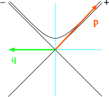
Figure 19: Reference frame for the analysis of deeply inelastic scattering.

For this purpose, we define a convenient reference frame, which is illustrated in Fig. 19. Denoting components of vectors $v^{\mu}$ by $(v^{+},v^{-},{\bf v}_{T})$, we chose the frame in which

$$(q^{+},q^{-},{\bf q})={1\over\sqrt{2}}\ (-Q,Q,{\bf 0}).$$ (64)

We also demand that the transverse components of the hadron momentum be zero in our frame. Then

$$(p^{+},p^{-},{\bf p})\approx{1\over\sqrt{2}}\ ({Q\over x_{\rm bj}},{x_{\rm bj}m_{h}^{2}\over Q},{\bf 0}).$$ (65)

Notice that in the chosen reference frame the hadron momentum is big and the momentum transfer is big.

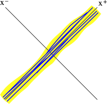
Figure 20: Interactions within a fast moving hadron. The lines represent world lines of quarks and gluons. The interaction points are spread out in $x^{+}$ and pushed together in $x^{-}$.

Consider the interactions among the quarks and gluons inside a hadron, using $x^{+}$ in the role of “time” as in Section 2.3. For a hadron at rest, these interactions happen in a typical time scale $\Delta x^{+}\sim 1/m$, where $m\sim 300\ {\ \rm MeV}$. A hadron that will participate in a deeply inelastic scattering event has a large momentum, $p^{+}\sim Q$, in the reference frame that we are using. The Lorentz transformation from the rest frame spreads out interactions by a factor $Q/m$, so that

$$\Delta x^{+}\sim{1\over m}\times{{Q\over m}}={Q\over m^{2}}.$$ (66)

This is illustrated in Fig. 20.

I offer two caveats here. First, I am treating $x_{\rm bj}$ as being of order 1. To treat small $x_{\rm bj}$ physics, one needs to put back the factors of $x_{\rm bj}$, and the picture changes rather dramatically. Second, the interactions among the quarks and gluons in a hadron at rest can take place on time scales $\Delta x^{+}$ that are much smaller than $1/m$, as we discussed in Section 3. We will discuss this later on, but for now we start with the simplest picture.

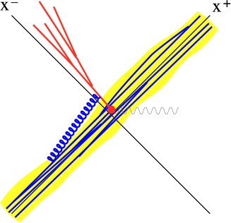
Figure 21: The virtual photon meets the fast moving hadron. One of the partons is annihilated and recreated as a parton with a large minus component of momentum. This parton develops into a jet of particles.

What happens when the fast moving hadron meets the virtual photon? The interaction with the photon carrying momentum $q^{-}\sim Q$ is localized to within

$$\Delta x^{+}\sim{1/Q}.$$ (67)

During this short time interval, the quarks and gluons in the proton are effectively free, since their typical interaction times are comparatively much longer.

We thus have the following picture. At the moment $x^{+}$ of the interaction, the hadron effectively consists of a collection of quarks and gluons (partons) that have momenta $(p_{i}^{+},{\bf p}_{i})$. We can treat the partons as being free. The $p_{i}^{+}$ are large, and it is convenient to describe them using momentum fractions $\xi_{i}$:

$${\xi_{i}=p_{i}^{+}/p^{+}},\hskip 28.45274pt0<\xi_{i}<1.$$ (68)

(This is convenient because the $\xi_{i}$ are invariant under boosts along the $z$ axis.) The transverse momenta of the partons, ${\bf p}_{i}$, are small compared to $Q$ and can be neglected in the kinematics of the $\gamma$-parton interaction. The “on-shell” or “kinetic” minus momenta of the partons, $p_{i}^{-}={\bf p}_{i}^{2}/(2p_{i}^{+})$, are also very small compared to $Q$ and can be neglected in the kinematics of the $\gamma$-parton interaction. We can think of the partonic state as being described by a wave function

$$\psi(p_{1}^{+},{\bf p}_{1};p_{2}^{+},{\bf p}_{2};\cdots),$$ (69)

where indices specifying spin and flavor quantum numbers have been suppressed.

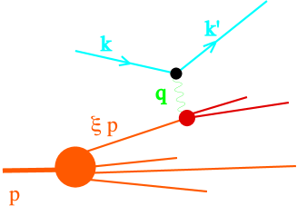
Figure 22: Feynman diagram for deeply inelastic scattering.

This approximate picture is represented in Feynman diagram language in Fig. 22. The larger filled circle represents the hadron wave function $\psi$. The smaller filled circle represents a sum of subdiagrams in which the particles have virtualities of order $Q^{2}$. All of these interactions are effectively instantaneous on the time scale of the intra-hadron interactions that form the wave function. The approximate picture also leads to an intuitive formula that relates the observed cross section to the cross section for $\gamma$-parton scattering:

$${{d\sigma}\over dE^{\prime}\,d\omega^{\prime}}\sim\int_{0}^{1}\!d\xi\sum_{a}\ {f_{\!a/h}\!(\xi,\mu_{F})}\ {{d\hat{\sigma}}_{\!a}(\mu_{F})\over dE^{\prime}\,d\omega^{\prime}}+{\cal O}(m/Q).$$ (70)

In Eq. (70), the function $f$ is a parton distribution function: ${f_{\!a/h}\!(\xi,\mu_{F})}\ d\xi$ gives probability to find a parton with flavor $a=g,u,\bar{u},d,\dots$ in hadron $h$, carrying momentum fraction within $d\xi$ of $\xi=p_{i}^{+}/p^{+}$. If we knew the wave functions $\psi$, we would form $f$ by summing over the number $n$ of unobserved partons, integrating $|\psi_{n}|^{2}$ over the momenta of the unobserved partons, and also integrating over the transverse momentum of the observed parton.

The second factor in Eq. (70), ${{d\hat{\sigma}}_{\!a}/dE^{\prime}\,d\omega^{\prime}}$, is the cross section for scattering the lepton from the parton of flavor $a$ and momentum fraction $\xi$.

I have indicated a dependence on a factorization scale $\mu_{F}$ in both factors of Eq. (70). This dependence arises from the existence of virtual processes among the partons that take place on a time scale much shorter than the nominal $\Delta x^{+}\sim Q/m^{2}$. I will discuss this dependence in some detail shortly.

4.4 The hard scattering cross section

The parton distribution functions in Eq. (70) are derived from experiment. The hard scattering cross sections ${{d\hat{\sigma}}_{\!a}(\mu)/dE^{\prime}\,d\omega^{\prime}}$ are calculated in perturbation theory, using diagrams like those shown in Fig. 23. The diagram on the left is the lowest order diagram. The diagram on the right is one of several that contributes to $d\hat{\sigma}$ at order $\alpha_{s}$; in this diagram the parton $a$ is a gluon.

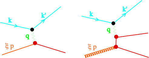
         Lowest order.                      Higher order.

Figure 23: Some Feynman diagrams for the hard scattering part of deeply inelastic scattering.

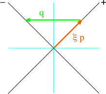
Figure 24: Kinematics of lowest order diagram.

One can understand a lot about deeply inelastic scattering from Fig. 24, which illustrates the kinematics of the lowest order diagram. Recall that in the reference frame that we are using, the virtual vector boson has zero transverse momentum. The incoming parton has momentum along the plus axis. After the scattering, the parton momentum must be on the cone $k_{\mu}k^{\mu}=0$, so the only possibility is that its minus momentum is non-zero and its plus momentum vanishes. That is

$$\xi p^{+}+q^{+}=0.$$ (71)

Since $p^{+}=Q/(x_{\rm bj}\sqrt{2})$ while $q^{+}=-Q/\sqrt{2}$, this implies

$${\xi=x_{\rm bj}}.$$ (72)

The consequence of this is that the lowest order contribution to $d\hat{\sigma}$ in Eq. (70) contains a delta function that sets $\xi$ to $x_{\rm bj}$. Thus deeply inelastic scattering at a given value of $x_{\rm bj}$ provides a determination of the parton distribution functions at momentum fraction $\xi$ equal to $x_{\rm bj}$, as long as one works only to leading order. In fact, because of this close relationship, there is some tendency to confuse the structure functions $F_{n}(x_{\rm bj},Q^{2})$ with the parton distribution functions $f_{a,h}(\xi,\mu_{F})$. I will try to keep these concepts separate: the structure functions $F_{n}$ are something that one measures directly in deeply inelastic scattering; the parton distribution functions are determined rather indirectly from experiments like deeply inelastic scattering, using formulas that are correct only up to some finite order in $\alpha_{s}$.

4.5 Factorization for the structure functions

We will look at DIS in a little detail since it is so important. Our object is to derive a formula at lowest order in perturbation theory relating the measured structure functions for $e^{-}+h\to e^{-}+X$ via photon exchange and the parton distribution functions.

Start with Eq. (70), representing Fig. 22. We change variables in this equation from $(E^{\prime},\omega^{\prime})$ to $(x_{\rm bj},y)$. We relate $x_{\rm bj}$ to the momentum fraction $\xi$ and a new variable $\hat{x}$ that is just $x_{\rm bj}$ with the proton momentum $p^{\mu}$ replaced by the parton momentum $\xi p^{\mu}$:

$${x_{\rm bj}}={Q^{2}\over 2p\cdot q}=\xi\ {Q^{2}\over 2\xi p\cdot q}={\xi\hat{x}}.$$ (73)

That is, $\hat{x}$ is the parton level version of $x_{\rm bj}$. The variable $y$ is identical to the parton level version of $y$ because $p^{\mu}$ appears in both the numerator and denominator:

$$y={p\cdot q\over p\cdot k}={\xi p\cdot q\over\xi p\cdot k}.$$ (74)

Thus Eq. (70) becomes

$${d\sigma\over{dx_{\rm bj}}\,dy}\sim\int_{0}^{1}\!d\xi\sum_{a}\ f_{\!a/h}\!(\xi,\mu_{F})\ {1\over{\xi}}\left[{d\hat{\sigma}_{\!a}(\mu_{F})\over{d\hat{x}}\,dy}\right]_{\hat{x}=x_{\rm bj}/\xi}+{\cal O}(m/Q).$$ (75)

We can calculate $d\hat{\sigma}_{\!a}/({d\hat{x}}\,dy)$ in perturbation theory. At lowest order this is particularly simple, and we obtain results proportional to delta functions of $x_{\rm bj}/\xi$. Using Eq. (62) to relate $d\sigma/(dx_{\rm bj}dy)$ to the structure functions $F_{1}$ and $F_{2}$ for $\gamma$ exchange, we obtain the simple lowest order results

$${F_{1}}(x_{\rm bj},Q^{2})\sim{1\over 2}\sum_{a}\ Q_{a}^{2}\ {f_{\!a/h}\!(x_{\rm bj})}+{\cal O}(\alpha_{s})+{\cal O}(m/Q),$$ (76)

$${F_{2}}(x_{\rm bj},Q^{2})\sim\sum_{a}\ Q_{a}^{2}\ {x_{\rm bj}\,f_{\!a/h}\!(x_{\rm bj})}+{\cal O}(\alpha_{s})+{\cal O}(m/Q).$$ (77)

The factor 1/2 between $x_{\rm bj}F_{1}$ and $F_{2}$ follows from the Feynman diagrams for spin 1/2 quarks.

4.6 $\mu_{F}$ dependence

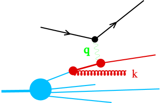
Figure 25: Deeply inelastic scattering with a gluon emission.

I have so far presented a rather simplified picture of deeply inelastic scattering in which the hard scattering takes place on a time scale $\Delta x^{+}\sim 1/Q$, while the internal dynamics of the proton take place on a much longer time scale $\Delta x^{+}\sim Q/m^{2}$. What happens when one actually computes Feynman diagrams and looks at what time scales contribute? Consider the graph shown in Fig. 25. One finds that the transverse momenta ${\bf k}$ range from order $m$ to order $Q$, corresponding to energy scales $k^{-}={\bf k}^{2}/2k^{+}$ between $k^{-}\sim m^{2}/Q$ and $k^{-}=Q^{2}/Q\sim Q$, or time scales $Q/m^{2}\ \hbox{\raise 2.0pt\hbox{$<$} \kern-13.0pt\lower 3.0pt\hbox{$\sim$}}\ \Delta x^{+}\ \hbox{\raise 2.0pt\hbox{$<$} \kern-13.0pt\lower 3.0pt\hbox{$\sim$}}\ 1/Q$.

The property of factorization for the cross section of deeply inelastic scattering, embodied in Eq. (70), is established by showing that the perturbative expansion can be rearranged so that the contributions from long time scales appear in the parton distribution functions, while the contributions from short time scales appear in the hard scattering functions. (See Ref. [24] for more information.) Thus, in Fig. 25, a gluon emission with ${\bf k}^{2}\sim m^{2}$ is part of ${f(\xi)}$, while a gluon emission with ${\bf k}^{2}\sim Q^{2}$ is part of ${d\hat{\sigma}}$.

Breaking up the cross section into factors associated with short and long time scales requires the introduction of a factorization scale, $\mu_{F}$. When calculating the diagram in Fig. 25, one integrates over $\bf k$. Roughly speaking, one counts the contribution from ${\bf k}^{2}<\mu_{F}^{2}$ as part of the higher order contribution to $f_{a/h}(\xi,\mu_{F})$, convoluted with the lowest order hard scattering function $d\hat{\sigma}$ for deeply inelastic scattering from a quark. The contribution from $\mu_{F}^{2}<{\bf k}^{2}$ then counts as part of the higher order contribution to $d\hat{\sigma}$ convoluted with an uncorrected parton distribution. This is illustrated in Fig. 26. (In real calculations, the split is accomplished with the aid of dimensional regularization, and is a little more subtle than a simple division of the integral into two parts.)

Figure 26: Time scales in factorization.

A consequence of this is that both ${{d\hat{\sigma}_{\!a}(\mu_{\!F})/dE^{\prime}\,d\omega^{\prime}}}$ and ${f_{\!a/h}(\xi,\mu_{\!F})}$ depend on $\mu_{\!F}$. Thus we have two scales, the factorization scale $\mu_{F}$ in $f_{\!f/h}(\xi,\mu_{\!F})$ and the renormalization scale $\mu$ in $\alpha_{s}(\mu)$. (When we expand $d\hat{\sigma}$ in powers of $\alpha_{s}(\mu)$ then the coefficients depend on $\mu$.) As with $\mu$, the cross section does not depend on $\mu_{F}$. Thus there is an equation $d({\it cross\ section})/d\mu_{F}=0$ that is satisfied to the accuracy of the perturbative calculation used. If you work harder and calculate to higher order, then the dependence on $\mu_{F}$ is less.

Often one sets $\mu_{F}=\mu$ in applied calculations. In fact, it is rather common in applications to deeply inelastic scattering to set $\mu_{F}=\mu=Q$.

4.7 Contour graphs of scale dependence

As an example, look at the one jet inclusive cross section in proton-antiproton collisions. Specifically, consider the cross section $d\sigma/dE_{T}d\eta$ to make a collimated spray of particles, a jet, with transverse energy $E_{T}$ and rapidity $\eta$. (Here $E_{T}$ is essentially the transverse momentum carried by the particles in the jet and $\eta$ is related to the angle between the jet and the beam direction by $\eta\equiv\ln(\tan(\theta/2)$). We will investigate this process and discuss the definitions in the next section. For now, all we need to know is that the theoretical formula for the cross section at next-to-leading order involves the strong coupling $\alpha_{s}(\mu)$ and two factors $f_{a/h}(x,\mu_{F})$ representing the distribution of partons in the two incoming hadrons. There is a parton level hard scattering cross section that also depends on $\mu$ and $\mu_{F}$.

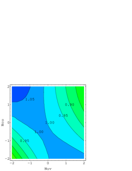
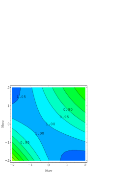
         $E_{T}=100{\ \rm GeV}$                          $E_{T}=500{\ \rm GeV}$

Figure 27: Contour plots of the one jet inclusive cross section versus the renormalization scale $\mu$ and the factorization scale $\mu_{F}$. The cross section is $d\sigma/dE_{T}d\eta$ at $\eta=0$ with $E_{T}=100\ {\ \rm GeV}$ in the first graph and $E_{T}=500\ {\ \rm GeV}$ in the second. The horizontal axis in each graph represents $N_{UV}\equiv\log_{2}(2\mu/E_{T})$ and the vertical axis represents $N_{CO}\equiv\log_{2}(2\mu_{F}/E_{T})$. The contour lines show 5% changes in the cross section relative to the cross section at the center of the figures. The c.m energy is $\sqrt{s}=1800\ {\ \rm GeV}$.

How does the cross section depend on $\mu$ in $\alpha_{s}(\mu)$ and $\mu_{F}$ in $f_{a/h}(x,\mu_{F})$? In Fig. 27, I show contour plots of the jet cross section versus $\mu$ and $\mu_{F}$ at two different values of $E_{T}$. The center of the plots corresponds to a standard choice of scales, $\mu=\mu_{F}=E_{T}/2$. The axes are logarithmic, representing $\log_{2}(2\mu/E_{T})$ and $\log_{2}(2\mu_{F}/E_{T})$. Thus $\mu$ and $\mu_{F}$ vary from $E_{T}/8$ to $2E_{T}$ in the plots.

Notice that the dependence on the two scales is rather mild for the next-to-leading order cross section. The cross section calculated at leading order is quite sensitive to these scales, but most of the scale dependence found at order $\alpha_{s}^{2}$ has been canceled by the $\alpha_{s}^{3}$ contributions to the cross section. One reads from the figure that the cross section varies by roughly ${\pm 15\%}$ in the central region of the graphs, both for medium and large $E_{T}$. Following the argument of Sec. 3.4, this leads to a rough estimate of 15% for the theoretical error associated with truncating perturbation theory at next-to-leading order.

4.8  MS  definition of parton distribution functions

The factorization property, Eq. (70), of the deeply inelastic scattering cross section states that the cross section can be approximated as a convolution of a hard scattering cross section that can be calculated perturbatively and parton distribution functions $f_{a/A}(x,\mu_{F})$. But what are the parton distribution functions? This question has some practical importance. The hard scattering cross section is essentially the physical cross section divided by the parton distribution function, so the precise definition of the parton distribution functions leads to the rules for calculating the hard scattering functions.

The definition of the parton distribution functions is to some extent a matter of convention. The most commonly used convention is the  MS  definition, which arose from the theory of deeply inelastic scattering in the language of the “operator product expansion”[25]. Here I will follow the (equivalent) formulation of Ref. [14]. For a more detailed pedagogical review, the reader may consult Ref. [26].

Using the  MS  definition, the distribution of quarks in a hadron is given as the hadron matrix element of certain quark field operators:

$${f_{i/h}(\xi,\mu_{F})}={1\over 2}\int{dy^{-}\over 2\pi}\ e^{-i\xi p^{+}y^{-}}\langle p|{\bar{\psi}}_{i}(0,y^{-},{\bf 0})\gamma^{+}{F}{\psi}_{i}(0)|p\rangle.$$ (78)

Here $|p\rangle$ represents the state of a hadron with momentum $p^{\mu}$ aligned so that $p_{T}=0$. For simplicity, I take the hadron to have spin zero. The operator $\psi(0)$, evaluated at $x^{\mu}=0$, annihilates a quark in the hadron. The operator ${\bar{\psi}}_{i}(0,y^{-},{\bf 0})$ recreates the quark at $x^{+}={\bf x}_{T}=0$ and $x^{-}=y^{-}$, where we take the appropriate Fourier transform in $y^{-}$ so that the quark that was annihilated and recreated has momentum $k^{+}=\xi p^{+}$. The motivation for the definition is that this is the hadron matrix element of the appropriate number operator for finding a quark.

There is one subtle point. The number operator idea corresponds to a particular gauge choice, $A^{+}=0$. If we are using any other gauge, we insert the operator

$${F}={\cal P}\exp\left(-ig\int_{0}^{y^{-}}dz^{-}{A}_{a}^{+}(0,z^{-},{\bf 0})\,t_{a}\right).$$ (79)

The ${\cal P}$ indicates a path ordering of the operators and color matrices along the path from $(0,0,{\bf 0})$ to $(0,y^{-},{\bf 0})$. This operator is the identity operator in $A^{+}=0$ gauge and it makes the definition gauge invariant.

    

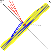
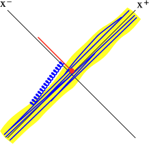
         DIS                  Parton distribution

Figure 28: Deeply inelastic scattering and the parton distribution functions.

The physics of this definition is illustrated in Fig. 28. The first picture (from Fig. 21) illustrates the amplitude for deeply inelastic scattering. The fast proton moves in the plus direction. A virtual photon knocks out a quark, which emerges moving in the minus direction and develops into a jet of particles. The second picture illustrates the amplitude associated with the quark distribution function. We express $F$ as $F_{2}F_{1}$ where

$${F_{2}} = \bar{\cal P}\exp\left(+ig\int^{\infty}_{y^{-}}\!\!dz^{-}{A}_{a}^{+}(0,z^{-},{\bf 0})\,t_{a}\right),$$

$${F_{1}} = {\cal P}\exp\left(-ig\int_{0}^{\infty}\!\!dz^{-}{A}_{a}^{+}(0,z^{-},{\bf 0})\,t_{a}\right).$$ (80)

and write the quark distribution function including a sum over intermediate states $|N\rangle$:

$${f_{i/h}(\xi,\mu_{F})}={1\over 2}\int{dy^{-}\over 2\pi}\ e^{-i\xi p^{+}y^{-}}\sum_{N}\langle p|{\bar{\psi}}_{i}(0,y^{-},{\bf 0})\gamma^{+}{F_{2}}|N\rangle\langle N|{F_{1}}{\psi}_{i}(0)|p\rangle.$$ (81)

Then the amplitude depicted in the second picture in Fig. 28 is $\langle N|{F_{1}}{\psi}_{i}(0)|p\rangle$. The operator $\psi$ annihilates a quark in the proton. The operator $F_{1}$ stands in for the quark moving in the minus direction. The gluon field $A$ evaluated along a lightlike line in the minus direction absorbs longitudinally polarized gluons from the color field of the proton, just as the real quark in deeply inelastic scattering can do. Thus the physics of deeply inelastic scattering is built into the definition of the quark distribution function, albeit in an idealized way. The idealization is not a problem because the hard scattering function $d\hat{\sigma}$ systematically corrects for the difference between real deeply inelastic scattering and the idealization.

There is one small hitch. If you calculate any Feynman diagrams for ${f_{i/h}(\xi,\mu_{F})}$, you are likely to wind up with an ultraviolet-divergent integral. The operator product that is part of the definition needs renormalization. This hitch is only a small one. We simply agree to do all of the renormalization using the  MS  scheme for renormalization. It is this renormalization that introduces the scale $\mu_{F}$ into ${f_{i/h}(\xi,\mu_{F})}$. This role of $\mu_{F}$ is in accord with Fig. 26: roughly speaking $\mu_{F}$ is the upper cutoff for what momenta belong with the parton distribution function; at the same time it is the lower cutoff for what momenta belong with the hard scattering function.

What about gluons? The definition of the gluon distribution function is similar to the definition for quarks. We simply replace the quark field $\psi$ by suitable combinations of the gluon field $A^{\mu}$, as described in Refs. [14] and [26].

4.9 Evolution of the parton distributions

Since we introduced a scale $\mu_{F}$ in the definition of the parton distributions in order to define their renormalization, there is a renormalization group equation that gives the $\mu_{F}$ dependence

$${d\over d\ln\mu_{F}}f_{a/h}(x,\mu_{F})=\sum_{b}\int_{x}^{1}{d\xi\over\xi}\ P_{ab}(x/\xi,\alpha_{s}(\mu_{F}))\ f_{b/h}(\xi,\mu_{F}).$$ (82)

This is variously known as the evolution equation, the Altarelli-Parisi equation, and the DGLAP (Dokshitzer-Gribov-Lipatov-Altarelli-Parisi) equation. Note the sum over parton flavor indices. The evolution of, say, an up quark ($a=u$) can involve a gluon ($b=g$) through the element $P_{ug}$ of the kernel that describes gluon splitting into $\bar{u}u$.

The equation is illustrated in Fig. 29. When we change the renormalization scale $\mu_{F}$, the change in the probability to find a parton with momentum fraction $x$ and flavor $a$ is proportional to the probability to find such a parton with large transverse momentum. The way to get this parton with large transverse momentum is for a parton carrying momentum fraction $\xi$ and much smaller transverse momentum to split into partons carrying large transverse momenta, including the parton that we are looking for. This splitting probability, integrated over the appropriate transverse momentum ranges, is the kernel $P_{ab}$.

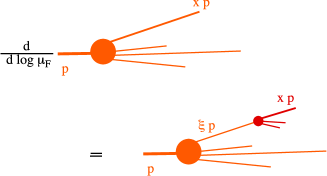
Figure 29: The renormalization group equation for the parton distribution functions.

The kernel $P$ in Eq. (82) has a perturbative expansion

$$P_{ab}(x/\xi,\alpha_{s}(\mu_{F}))=P_{ab}^{(1)}(x/\xi)\ {\alpha_{s}(\mu_{F})\over\pi}+P_{ab}^{(2)}(x/\xi)\ \left({\alpha_{s}(\mu_{F})\over\pi}\right)^{2}+\cdots.$$ (83)

The first two terms are known and are typically used in numerical solutions of the equation. To learn more about the DGLAP equation, the reader may consult Refs. [1] and [26].

4.10 Determination and use of the parton distributions

The  MS  definition giving the parton distribution in terms of operators is process independent – it does not refer to any particular physical process. These parton distributions then appear in the QCD formula for any process with one or two hadrons in the initial state. In principle, the parton distribution functions could be calculated by using the method of lattice QCD (see Ref. [26]). Currently, they are determined from experiment.

Currently the most comprehensive analyses are being done by the CTEQ [20] and MRS [27] groups. These groups perform a “global fit” to data from experiments of several different types. To perform such a fit one chooses a parameterization for the parton distributions at some standard factorization scale $\mu_{0}$. Certain sum rules that follow from the definition of the parton distribution functions are built into the parameterization. An example is the momentum sum rule:

$$\sum_{a}\int_{0}^{1}d\xi\ \xi\ f_{a/h}(\xi,\mu)=1.$$ (84)

Given some set of values for the parameters describing the $f_{a/h}(x,\mu_{0})$, one can determine $f_{a/h}(x,\mu)$ for all higher values of $\mu$ by using the evolution equation. Then the QCD cross section formulas give predictions for all of the experiments that are being used. One systematically varies the parameters in $f_{a/h}(x,\mu_{0})$ to obtain the best fit to all of the experiments. One source of information about these fits is the world wide web pages of Ref. [28].

If the freedom available for the parton distributions is used to fit all of the world’s data, is there any physical content to QCD? The answer is yes: there are lots of experiments, so this program won’t work unless QCD is right. In fact, there are roughly 1400 data in the CTEQ fit and only about 25 parameters available to fit these data.

5 QCD in hadron-hadron collisions

When there is a hadron in the initial state of a scattering process, there are inevitably long time scales associated with the binding of the hadron, even if part of the process is a short-time scattering. We have seen, in the case of deeply inelastic scattering of a lepton from a single hadron, that the dependence on these long time scales can be factored into a parton distribution function. But what happens when two high energy hadrons collide? The reader will not be surprised to learn that we then need two parton distribution functions.

I explore hadron-hadron collisions in this section. I begin with the definition of a convenient kinematical variable, rapidity. Then I discuss, in turn, production of vector bosons ($\gamma^{*}$, $W$, and $Z$) and jet production. The theory for the production of heavy quarks is similar and I omit it.

5.1 Kinematics: rapidity

In describing hadron-hadron collisions, it is useful to employ a kinematic variable $y$ that is called rapidity. Consider, for example, the production of a $Z$ boson plus anything, $p+\bar{p}\to Z+X$. Choose the hadron-hadron c.m. frame with the $z$ axis along the beam direction. In Fig. 30, I show a drawing of the collision. The arrows represent the momenta of the two hadrons; in the c.m. frame these momenta have equal magnitudes. We will want to describe the process at the parton level, $a+b\to Z+X$. The two partons $a$ and $b$ each carry some share of the parent hadron’s momentum, but generally these will not be equal shares. Thus the magnitudes of the momenta of the colliding partons will not be equal. We will have to boost along the $z$ axis in order to get to the parton-parton c.m. frame. For this reason, it is useful to use a variable that transforms simply under boosts. This is the motivation for using rapidity.

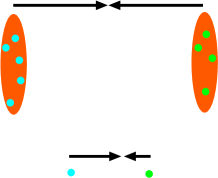
Figure 30: Collision of two hadrons containing partons producing a $Z$ boson. The c.m. frame of the two hadrons is normally $\it not$ the c.m. frame of the two partons that create the $Z$ boson.

Let $q^{\mu}=(q^{+},q^{-},{\bf q})$ be the momentum of the $Z$ boson. Then the rapidity of the $Z$ is defined as

$$y={1\over 2}\ln\!\left({q^{+}\over q^{-}}\right).$$ (85)

The four components $(q^{+},q^{-},{\bf q})$ of the $Z$ boson momentum can be written in terms of four variables, the two components of the $Z$ boson’s transverse momentum ${\bf q}$, its mass $M$, and its rapidity:

$$q^{\mu}=(e^{y}\sqrt{({\bf q}^{2}+M^{2})/2},\ e^{-y}\sqrt{({\bf q}^{2}+M^{2})/2},\ {\bf q}).$$ (86)

The utility of using rapidity as one of the variables stems from the transformation property of rapidity under a boost along the $z$ axis:

$$q^{+}\to e^{\omega}q^{+},\quad q^{-}\to e^{-\omega}q^{-},\quad{\bf q}\to{\bf q}.$$ (87)

Under this transformation,

$$y\to y+\omega.$$ (88)

This is as simple a transformation law as we could hope for. In fact, it is just the same as the transformation law for velocities in non-relativistic physics in one dimension.

Figure 31: Definition of the polar angle $\theta$ used in calculating the rapidity of a massless particle.

Consider now the rapidity of a massless particle. Let the massless particle emerge from the collision with polar angle $\theta$, as indicated in Fig. 31. A simple calculation relates the particle’s rapidity $y$ to $\theta$:

$$y=-\ln\left(\tan(\theta/2)\right)\,,\hskip 28.45274pt(m=0).$$ (89)

Another way of writing this is

$$\tan\theta=1/\sinh y\,,\hskip 28.45274pt(m=0).$$ (90)

One also defines the pseudorapidity $\eta$ of a particle, massless or not, by

$$\eta=-\ln\left(\tan(\theta/2)\right)\hskip 28.45274pt{\rm or}\hskip 28.45274pt\tan\theta=1/\sinh\eta.$$ (91)

The relation between rapidity and pseudorapidity is

$$\sinh\eta=\sqrt{1+m^{2}/q_{T}^{2}}\ \sinh y.$$ (92)

Thus, if the particle isn’t quite massless, $\eta$ may still be a good approximation to $y$.

5.2 $\gamma^{*}$, $W$, $Z$ production in hadron-hadron collisions

Consider the process

$$A+B\to Z+X,$$ (93)

where $A$ and $B$ are high energy hadrons. This process and the corresponding process in which a $W$ boson is produced are historically important because they are the processes by which the $W$ and $Z$ bosons were first observed [29].

Two features of this reaction are important for our discussion. First, the mass of the $Z$ boson is large compared to 1 GeV, so that a process with a small time scale $\Delta t\sim 1/M_{Z}$ must be involved in the production of the $Z$. At lowest order in the strong interactions, the process is $q+\bar{q}\to Z$. Here the quark and antiquark are constituents of the high energy hadrons. The second significant feature is that the $Z$ boson does not participate in the strong interactions, so that our description of the observed final state can be very simple.

In process (93), we allow the $Z$ boson to have any transverse momentum ${\bf q}$. (Typically, then, ${\bf q}$ will be much smaller than $M_{Z}$.) Since we integrate over $\bf q$ and the mass of the $Z$ boson is fixed, there is only one variable needed to describe the momentum of the $Z$ boson. We choose to use its rapidity $y$, so that we are interested in the cross section $d\sigma/dy$.

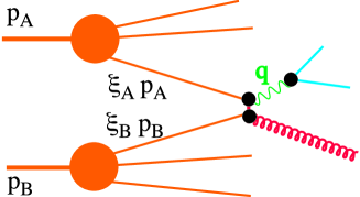
Figure 32: A Feynman diagram for $Z$ boson production in a hadron-hadron collision. Two partons, carrying momentum fractions $\xi_{A}$ and $\xi_{B}$, participate in the hard interaction. This particular Feynman diagram illustrates an order $\alpha_{s}$ contribution to the hard scattering cross section: a gluon is emitted in the process of making the $Z$ boson. The diagram also shows the decay of the $Z$ boson into an electron and a neutrino.

The cross section takes a factored form similar to that found for deeply inelastic scattering. Here, however, there are two parton distribution functions:

$${{d\sigma\over dy}}\approx\!\sum_{a,b}\int_{x_{A}}^{1}\!d\xi_{A}\int_{x_{B}}^{1}\!d\xi_{B}\ {f_{a/A}(\xi_{A},\mu_{F})}\ {f_{b/B}(\xi_{B},\mu_{F})}\ {{d\hat{\sigma}_{ab}(\mu_{F})\over dy}}.$$ (94)

The meaning of this formula is intuitive: ${f_{a/A}(\xi_{A},\mu_{F})}\,d\xi_{A}$ gives the probability to find a parton in hadron $A$; ${f_{b/B}(\xi_{B},\mu_{f})}\,d\xi_{B}$ gives the probability to find a parton in hadron $B$; ${{d\hat{\sigma}_{ab}/dy}}$ gives the cross section for these partons to produce the observed $Z$ boson. The formula is illustrated in Fig. 32. The hard scattering cross section can be calculated perturbatively. Fig. 32 illustrates one particular order $\alpha_{s}$ contribution to ${{d\hat{\sigma}_{ab}/dy}}$. The integrations over parton momentum fractions have limits $x_{A}$ and $x_{B}$, which are given by

$$x_{A}=e^{y}\sqrt{M^{2}/s},\quad\quad x_{B}=e^{-y}\sqrt{M^{2}/s}.$$ (95)

Eq. (94) has corrections of order $m/M_{Z}$, where $m$ is a mass characteristic of hadronic systems, say 1 GeV. In addition, when ${{d\hat{\sigma}_{ab}/dy}}$ is calculated to order $\alpha_{s}^{N}$, then there are corrections of order $\alpha_{s}^{N+1}$.

We could equally well talk about $A+B\to\gamma^{*}+X$ where the virtual photon decays into a muon pair or an electron pair that is observed and where the mass $Q$ of the $\gamma^{*}$ is large compared to 1 GeV. For $A+B\to\mu^{+}+\mu^{-}+X$ one has the formula

$${d\sigma\over dQ^{2}dy}=\sum_{a,b}\int_{x_{A}}^{1}\!d\xi_{A}\int_{x_{B}}^{1}\!d\xi_{B}\ {f_{a/A}(\xi_{A},\mu_{F})}\ {f_{b/B}(\xi_{B},\mu_{F})}\ {{d\hat{\sigma}_{ab}(\mu_{F})\over dQ^{2}dy}}.$$ (96)

This process is historically important. Before QCD, one had partons and QED. Partons and QED did a good job of explaining deeply inelastic scattering. But there were other ways to explain deeply inelastic scattering. High mass dimuon production was investigated experimentally by Lederman et al. [30] Drell and Yan [31] proposed to explain the experimental results using the lowest order version of the formula above. It worked. The alternative methods that worked for deeply inelastic scattering did not work here. This helped to establish the parton picture.

5.3 Factorization is not so obvious

The factorization formula Eq. (94) is supposed to hold up to $m^{2}/Q^{2}$ corrections. This result is not so obvious, and in fact does not hold graph by graph. A graph for which it does not hold is shown in Fig. 33. Does factorization hold if one sums over graphs? The answer is yes, but to show this one needs to use unitarity, causality and gauge invariance. For more information, the reader is invited to consult Ref. [24].

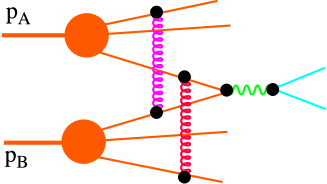
Figure 33: A graph for which factorization does not work. The spectator partons interact softly with the active partons, so that the soft part of the graph does not break up into two factors.

5.4 Jet production

In our study of high energy electron-positron annihilation, we discovered three things. First, QCD makes the qualitative prediction that particles in the final state should tend to be grouped in collimated sprays of hadrons called jets. The jets carry the momenta of the first quarks and gluons produced in the hard process. Second, certain kinds of experimental measurements probe the short-time physics of the hard interaction, while being insensitive to the long-time physics of parton splitting, soft gluon exchange, and the binding of partons into hadrons. Such measurements are called infrared safe. Third, among the infrared safe observables are cross sections to make jets.

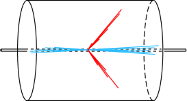
Figure 34: Sketch of a two-jet event at a hadron collider. The cylinder represents the detector, with the beam pipe along its axis. Typical hadron-hadron collisions produce beam remnants, the debris from soft interactions among the partons. The particles in the beam remnants have small transverse momenta, as shown in the sketch. In rare events, there is a hard parton-parton collision, which produces jets with high transverse momenta. In the event shown, there are two high $P_{T}$ jets.

These ideas work for hadron-hadron collisions too. In such collisions, there is sometimes a hard parton-parton collision, which produces two or more jets, as depicted in Fig. 34. Consider the cross section to make one jet plus anything else,

$$A+B\to jet+X.$$ (97)

Let $E_{T}$ be the transverse energy of the jet, defined as the sum of the absolute values of the transverse momenta of the particles in the jet. Let $y$ be the rapidity of the jet. Given a definition of exactly what it means to have a jet with transverse energy $E_{T}$ and rapidity $y$, the jet production cross section takes the familiar factored form

$${d\sigma\over dE_{T}d\eta} \approx \sum_{a,b}\int_{x_{A}}^{1}\!\!\!d\xi_{A}\!\int_{x_{B}}^{1}\!\!\!d\xi_{B}\,{f_{a/A}(\xi_{A},\mu_{F})}\,{f_{b/B}(\xi_{B},\mu_{F})}\,{{{d\hat{\sigma}^{ab}(\mu_{F})\over dE_{T}d\eta}}}.$$ (98)

One diagram that contributes to $d\hat{\sigma}$ at next-to-leading order is shown in Fig. 35.

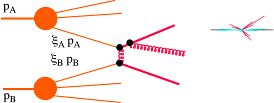
Figure 35: A Feynman diagram for jet production in hadron-hadron collisions. The leading order diagrams for $A+B\to jet+X$ occur at order $\alpha_{s}^{2}$. This particular diagram is for an interaction of order $\alpha_{s}^{3}$. When the emitted gluon is not soft or nearly collinear to one of the outgoing quarks, this diagram corresponds to a final state like that shown in the small sketch, with three jets emerging in addition to the beam remnants. Any of these jets can be the jet that is measured in the one jet inclusive cross section.

What shall we choose for the definition of a jet? At a crude level, high $E_{T}$ jets are quite obvious and the precise definition hardly matters. However, if we want to make a quantitative measurement of a jet cross section to compare to next-to-leading order theory, then the definition does matter. There are several possibilities for a definition that is infrared safe. The one most used in hadron-hadron collisions is based on cones. Here I will present a different algorithm that is similar to the algorithms used to define jets in electron-positron annihilation.

5.5 $k_{T}$ algorithm

The main idea of the $k_{T}$ algorithm [32] is to modify one of the algorithms used in $e^{+}e^{-}$ annihilation so that we use $E_{T}$, $\eta$ and $\phi$ as variables and to avoid contamination by the many low $E_{T}$ particles in the event. We choose a merging parameter $R$. Then we start with a list of “protojets” with momenta $p_{1}^{\mu},\dots,p_{N}^{\mu}$ as illustrated in Fig. 36. We also start with an empty list of finished jets. The end result is a list of momenta $p_{k}$ of finished jets, ordered in $E_{T}$.

Figure 36: A two jet event in a proton antiproton collision. The two protojets on the lower left are the first to be combined.

The algorithm can be stated very simply. See Fig. 36.

1. For each pair of protojets define

   $$d_{ij}=\min(E_{T,i}^{2},E_{T,j}^{2})\,[(\eta_{i}-\eta_{j})^{2}+(\phi_{i}-\phi_{j})^{2}]/R^{2}.$$ (99)

   For each protojet define

   $$d_{i}=E_{T,i}^{2}.$$ (100)

2. Find the smallest of all the $d_{ij}$ and the $d_{i}$. Call it $d_{\rm min}$.

3. If $d_{\rm min}$ is a $d_{ij}$, merge protojets $i$ and $j$ into a new protojet $k$ with

   $$E_{T,k} = E_{T,i}+E_{T,j}$$

   $$\eta_{k} = [E_{T,i}\,\eta_{i}+E_{T,j}\,\eta_{j}]/E_{T,k}$$

   $$\phi_{k} = [E_{T,i}\,\phi_{i}+E_{T,j}\,\phi_{j}]/E_{T,k}$$ (101)

4. If $d_{\rm min}$ is a $d_{i}$, then protojet $i$ is “not mergable.” Remove it from the list of protojets and add it to the list of jets.

5. If protojets remain, go to 1.

Evidently, if two protojets are collinear, they will be merged right away. If one has vanishing momentum, it will either get merged with a protojet nearby in angle, or it will become a low $E_{T}$ jet in the final list. Many of the jets have small $E_{T}$ and are really minijets, or just part of low $E_{T}$ debris. For an inclusive cross section to make $n$ high $E_{T}$ jets plus anything else, the many low $E_{T}$ jets do not affect the result. For an exclusive $n$ jet cross section, one would use a cutoff $E_{T,\rm min}$. Thus in either case, low $E_{T}$ particles do not change the result. Thus the algorithm is infrared safe.

6 Epilogue

QCD is a rich subject. The theory and the experimental evidence indicate that quarks and gluons interact weakly on short time and distance scales. But the net effect of these interactions extending over long time and distance scales is that the chromodynamic force is strong. Quarks are bound into hadrons. Outgoing partons emerge as jets of hadrons, with each jet composed of subjets. Thus QCD theory can be viewed as starting with simple perturbation theory, but it does not end there. The challenge for both theorists and experimentalists is to extend the range of phenomena that we can relate to the fundamental theory.

References

- [1] G. Sterman et al., Handbook of Perturbative QCD, Rev. Mod. Phys. 67, 157 (1995).
- [2] R. K. Ellis, W. J. Stirling, and B. R. Webber, QCD and Collider Physics, (Cambridge University Press, Cambridge, 1996).
- [3] L. Brown, Quantum Field Theory, (Cambridge University Press, Cambridge, 1992)
- [4] G. Sterman, An Introduction to Quantum Field Theory, (Cambridge University Press, Cambridge, 1993).
- [5] M. Peskin and D. V. Schroeder, An Introduction to Quantum Field Theory, (Addison-Wesley, Reading, 1995).
- [6] S. Weinberg, The Quantum Theory of Fields, (Cambridge University Press, Cambridge, 1995).
- [7] D. E. Soper, ed., QCD and Beyond, Proceedings of the 1995 Theoretical Advanced Studies Institute, Boulder, 1995, (World Scientific, Singapore, 1996).
- [8] D. E. Soper, Basics of QCD Perturbation Theory, e-Print Archive: hep-ph/9702203, in The Strong Interaction, from Hadrons to Partons, XXIV SLAC Summer Institute on Particle Physics Stanford, August 1996, edited by L. DePorcel (SLAC, Stanford, 1997).
- [9] G. Sterman, Phys. Rev. D 17, 2773 (1978); 17, 2789 (1978).
- [10] J. C. Collins and D. E. Soper, Nucl. Phys. B 193, 381 (1981).
- [11] Z. Kunszt and D. E. Soper, Phys. Rev. D 46, 192 (1992).
- [12] C. L. Basham, L. S. Brown, S. D. Ellis, and S. T. Love, Phys. Rev. D 19, 2018 (1979).
- [13] S. Bethke, Z. Kunszt, D. E. Soper, and W. J. Stirling, Nucl. Phys. B 370, 310 (1992).
- [14] J. C. Collins and D. E. Soper, Nucl. Phys. B 194, 445 (1982). G. Curci, W. Furmanski and R. Petronzio, Nucl. Phys. B 175, 27 (1980).
- [15] J. C. Collins, Renormalization, (Cambridge University Press, Cambridge, 1984).
- [16] L. Surguladze and M. Samuel, Rev. Mod. Phys. 68, 259 (1996).
- [17] D. E. Soper and L. Surguladze, Phys. Rev. D 54, 4566 (1996).
- [18] P. M. Stevenson, Phys. Rev. D 23, 2916 (1981).
- [19] S. J. Brodsky, G. P. Lepage and P. MacKenzie, Phys. Rev. D 28, 228 (1983).
- [20] H. Lai et al., e-Print Archive hep-ph/9606399, Phys. Rev. D 55, (to be published).
- [21] CDF Collaboration (F. Abe al.), Phys. Rev. Lett. 77, 438 (1996); B. Flaugher, CDF Collaboration, Proceedings of the XI Topical Workshop on ppbar Collider Physics, Padova, Italy, May 1996.
- [22] D0 Collaboration: N. Varelas, Proceedings of the International Conference on High Energy Physics, Warsaw, July 1996.
- [23] J. Huston et al., Phys. Rev. Lett. 77, 444 (1996).
- [24] J. C. Collins, D. E. Soper, and G. Sterman, in Perturbative QCD, edited by A. Mueller, (World Scientific, Singapore, 1989).
- [25] W. A. Bardeen, A. J. Buras, D. W. Duke, and T Muta, Phys. Rev. D 18, 3998 (1978).
- [26] D. E. Soper, in M. Golterman et al. eds., Lattice ’96 International Symposium on Lattice Field Theory, St. Louis, June 1996 (Elsevier Science, Amsterdam, to be published).
- [27] A. D. Martin, R. G. Roberts, and W. J. Stirling, Phys. Lett. B 387, 419 (1996).
- [28] P. Anandam and D. E. Soper, “A Potpourri of Partons”,http://zebu.uoregon.edu/~parton/.
- [29] UA1 Collaboration (G. Arnison et al.), Phys. Lett. B 122, 103 (1983); UA2 Collaboration (G. Banner et al.), Phys. Lett. B 122, 476 (1983).
- [30] J. C. Christenson et al., Phys. Rev. Lett. 25, 1523 (1970).
- [31] S. D. Drell and T.-M. Yan, Ann. Phys. 66, 578 (1971).
- [32] S. D. Ellis and D. E. Soper, Phys. Rev. D 48, 3160 (1993).