DESY T-00-01
MZ-TH/00–53
PSI-PR-00-17

Abstract

We present an introduction into the basic concepts of the Standard Model, i.e. the gauge theories of the forces and the Higgs mechanism for generating masses. The Glashow-Salam-Weinberg theory of the electroweak interactions will be described in detail. The key experiments are reviewed, including the precision tests at high energies. Finally, the limitations and possible physics areas beyond the Standard Model are discussed.

To be published in ”Scattering”, P. Sabatier ed., Academic Press, London (2000).

1 Prologue

A most fundamental element of physics is the reduction principle. The large variety of macroscopic forms of matter can be traced back, according to this principle, to a few microscopic constituents which interact by a small number of basic forces. The reduction principle has guided the unraveling of the structure of physics from the macroscopic world through atomic and nuclear physics to particle physics. The laws of Nature are summarized in the Standard Model of particle physics (Gla 61, Sal 68, Wei 67, Fri 72). All experimental observations are compatible with this model at a level of very high accuracy. Not all building blocks of the model, however, have been experimentally established so far. In particular, the Higgs mechanism for generating the masses of the fundamental particles (Hig 64, Eng 64, Gur 64) which is a cornerstone of the system, still lacks experimental verification up to now, even though indirect indications support this mechanism quite strongly.

Even if all the elements of the Standard Model will be established experimentally in the near future, the model cannot be considered the ultima ratio of matter and forces. Neither the fundamental parameters, masses and couplings, nor the symmetry pattern can be derived; these elements are merely built into the model by hand. Moreover, gravity with a structure quite different from the electroweak and strong forces, is not coherently incorporated in the theory.

Despite this criticism, the Standard Model provides a valid framework for the description of Nature, probed from microscopic scales of order $10^{-16}$ cm up to cosmological distances of order $10^{+28}$ cm. The model therefore ranks among the greatest achievements of mankind in understanding Nature.

The Standard Model consists of three components:

1. The basic constituents of matter are leptons and quarks (Gel 64, Zwe 64) which are realized in three families of identical structure:
                                    leptons: $\nu_{e}$ $\nu_{\mu}$ $\nu_{\tau}$ $e^{-}$ $\mu^{-}$ $\tau^{-}$ quarks: $u$ $c$ $t$ $d$ $s$ $b$
The entire ensemble of these constituents has been identified experimentally. The least known properties of these constituents are the profile of the top quark, the mixing among the lepton states and the quark states, and in particular, the structure of the neutrino sector.

2. Four different forces act between the leptons and quarks:

The electromagnetic and weak forces are unified in the Standard Model. The fields associated with these forces, as well as the fields associated with the strong force, are spin-1 fields, describing the photon $\gamma$, the electroweak gauge bosons $W^{\pm}$ and $Z$, and the gluons $g$. The interactions of the force fields with the fermionic constituents of matter as well as their self-interactions are described by Abelian and non-Abelian $SU(3)\times SU(2)\times U(1)$ gauge theories (Wey 29, Yan 54). The experimental exploration of these fundamental gauge symmetries is far advanced in the sector of lepton/quark-gauge boson interactions, yet much less is known so far from experiment about the self-interactions of the force fields. The gravitational interaction is mediated by a spin-2 field, describing the graviton $G$, with a character quite different from spin-1 gauge fields. The gravity sector is attached ad hoc to the other sectors of the Standard Model, not properly formulated yet as a quantum phenomenon.

3. The third component of the Standard Model is the Higgs mechanism (Hig 64, Eng 64, Gur 64). In this sector of the theory, scalar fields interact with each other in such a way that the ground state acquires a non-zero field strength, breaking the electroweak symmetries spontaneously. The potential describing these self-interactions is displayed in Fig. 1. The interaction energies of electroweak gauge bosons, leptons and quarks with this field manifest themselves as non-zero masses of these particles. If this picture is correct, a scalar particle, the Higgs boson, should be observed with a mass of less than about 700 GeV, the final experimentum crucis of the Standard Model.

Figure 1: The Higgs potential of the Standard Model.

Experimental efforts extending over more than a century, have been crucial in developing these basic ideas to a coherent picture. The first elementary particle discovered at the end of the 19th century was the electron (Wie 97, Tho 97, Kau 97,97a), followed later by the other charged leptons, the $\mu$ (And 37) and $\tau$ leptons (Per 75). The first species of weakly interacting neutrinos, $\nu_{e}$, was found in the fifties (Rei 53), the others, $\nu_{\mu}$ (Dan 62) and $\nu_{\tau}$ (Pol 00), one and five decades later. The up, down and strange quarks were “seen” first in deep-inelastic electron- and neutrino-nucleon scattering experiments (Fri 72a, Eic 73), the discovery of the charm quark (Aub 74, Aug 74) marked what is called “November revolution” of particle physics. The bottom quark of the third family was isolated in the 70’s (Her 77) while the discovery of the top quark followed only recently (Abe 95, Aba 95).

The photon as the quantum associated with the electromagnetic field, was discovered when the photo-electric effect was interpreted theoretically (Ein 05), while the heavy electroweak bosons $W^{\pm}$, $Z$ have first been isolated in $p\bar{p}$ collisions (Arn 83, Ban 83, Arn 83a, Bag 83). Gluons as the carriers of the strong force were discovered in the fragmented form of hadron jets, generated in $e^{+}e^{-}$ annihilation at high energies (Bra 79, Bar 79, Ber 79).

Future experimental activities will focus, in the framework of the Standard Model, on the properties of the top quark, the non-Abelian gauge symmetry structure of the self-interactions among the force fields, and last not least, on the search of Higgs bosons and, if discovered, on the analysis of its properties. This experimental program is a continuing task at the existing collider facilities LEP2, HERA and Tevatron, and it will extend to the next-generation facilities, the $pp$ collider LHC (ATL 99, CMS 94), a prospective $e^{+}e^{-}$ linear collider (Zer 99, Acc 98, Mur 96) with beam energies in the TeV range, and a prospective muon-collider (Ank 99, Aut 99). Other experimental facilities will lead to a better understanding of the neutrino properties and map out the quark mixings.

2 Introduction

2.1 The path to the standard model of the electroweak interactions

The weak interactions of the elementary particles have been discovered in $\beta$-decay processes. They are described by an effective Lagrangian of current $\times$ current type (Fer 34), in which the weak currents are coherent superpositions of charged vector and axial-vector currents, accounting for the violation of parity. For the $\mu$-decay process $\mu^{-}\rightarrow e^{-}\bar{\nu}_{e}\nu_{\mu}$ the Lagrangian is defined as

$${\cal L}=\frac{G_{F}}{\sqrt{2}}\left[\bar{\nu}_{\mu}\gamma_{\lambda}\left(1-\gamma_{5}\right)\mu\right]\left[\bar{e}\gamma_{\lambda}\left(1-\gamma_{5}\right)\nu_{e}\right]$$ (1)

The overall strength of the interaction is measured by the Fermi coupling constant

$$G_{F}\simeq 1.17\times 10^{-5}~{}{\rm GeV}^{-2}$$ (2)

which carries the dimension of [mass$]^{-2}$.

The Fermi theory of the weak interactions can only be interpreted as an effective low-energy theory which cannot be extended to arbitrarily high energies. Applying this theory to the scattering process $\nu_{\mu}e^{-}\rightarrow\mu^{-}\nu_{e}$ at high energies, the scattering amplitude rises indefinitely with the square of the energy $E_{\rm cms}=\sqrt{s}$ in the center-of-mass system of the colliding particles:

$$f_{0}[\nu_{\mu}e^{-}\rightarrow\mu^{-}\nu_{e}]=\frac{G_{F}s}{2\sqrt{2}\pi}$$ (3)

However, as an $S$-wave scattering amplitude, $f_{0}$ must fulfill the unitarity condition $|f_{0}|^{2}\leq\Im mf_{0}$, leading to the upper limit $|\Re ef_{0}|\leq 1/2$. The theory can therefore not be applied at energies in excess of

$$s\leq\sqrt{2}\pi/G_{F}\sim(600~{}{\rm GeV})^{2}\,.$$ (4)

A simple line of arguments allows us to deduce the structure of the weak interactions from unitarity constraints (Lle 73, Cor 74) applied to a set of high-energy scattering processes. In this way the existence of charged and neutral vector bosons can be predicted, as well as the existence of a scalar particle, together with the properties of their interactions.

Figure 2: Diagrams for scattering processes with implications on unitarity constraints.

a) Charged $W^{\pm}$ Bosons. The unitarity problem described above can be solved by assuming the weak interactions to be mediated by the exchange of a heavy charged vector boson $W^{\pm}$ (Yuk 35), cf. Fig. 2(a). The $W$ propagator damps the rise in the energy of the scattering amplitude:

$$f_{0}[\nu_{\mu}e^{-}\rightarrow\mu^{-}\nu_{e}]\rightarrow\frac{G_{F}s}{2\sqrt{2}\pi}\,\frac{M_{W}^{2}}{M_{W}^{2}-s}$$ (5)

which is compatible with the unitarity limit if the $W$-boson mass is sufficiently light. Defining the dimensionless coupling between the $W$-field and the weak current by $g_{W}/2\sqrt{2}$, the connection to Fermi’s theory at low energies leads to the relation $G_{F}/\sqrt{2}=g_{W}^{2}/8M_{W}^{2}$. If the coupling $g_{W}$ is of the same order as the electromagnetic $e$, the mass of the $W$ boson is close to 100 GeV. The weak interactions in this picture are therefore not really weak but their strength is reduced only by the short-range character of the $W$-exchange mechanism at low energies. The interaction is effectively weak since it is confined to distances of order $\lambda_{W}=M^{-1}_{W}$ where $\lambda_{W}$ is the small Compton wavelength of the $W$ boson.

b) Neutral $W^{3}$ Boson. Induced by the $\ell\nu_{\ell}W^{\pm}$ couplings, the theory predicts the production of $W^{+}W^{-}$ pairs in $e^{+}e^{-}$ annihilation. With the ingredients introduced up to this point, this process is mediated by the exchange of a neutrino, cf. Fig. 2(b). When the $W$ bosons in the final state are polarized longitudinally, their wave-functions $e_{\mu}(k)=(k^{3},0,0,k^{0})/M_{W}$ grow linearly with the energy. The scattering amplitude for the process $e^{+}e^{-}\rightarrow W^{+}W^{-}$, if mediated solely by $\nu_{e}$ exchange, therefore grows quadratically for high energies, and it violates the unitarity limit eventually. This divergence can be damped by the exchange of a doubly charged lepton in the $u$-channel, or else by the exchange of a neutral vector boson $W^{3}$ in the $s$-channel. Following the second branch, a trilinear coupling of the three $W$ bosons, $W^{\pm}=(W^{1}\mp iW^{2})/\sqrt{2}$ and $W^{3}$, must be introduced with strength $g_{W}\varepsilon_{klm}$. The couplings $g_{W}I^{k}_{ab}$ between the leptons $a,b$ and the $W$ bosons $k$, and the trilinear self-couplings $g_{W}\varepsilon_{klm}$ of the $W$ bosons must fulfill the consistency conditions

$$\left[I^{k},I^{l}\right]=i\varepsilon_{klm}I^{m}$$ (6)

to restore unitarity at high energies.

c) $W$ Self-Interactions. As a result of the trilinear couplings among the $W$ bosons, the $W$ bosons can scatter quasi-elastically, $WW\rightarrow WW$, cf. Fig. 2(c). The amplitude for the scattering of longitudinally polarized $W$ bosons, built-up by virtual $W$ exchanges, grows as the fourth power of $\sqrt{s}$ for high energies. This leading divergence is canceled by introducing a quadrilinear coupling among the $W$ bosons which must be of second order in $g_{W}$, and the dependence on the charge indices given by the tensors

$$\lambda_{klmn}=g_{W}^{2}\varepsilon_{klp^{\prime}}\varepsilon_{p^{\prime}mn}$$ (7)

However, unitarity is not yet completely restored for asymptotic energies since the amplitude still grows quadratically in the energy.

d) The Higgs Boson. Since all intrinsic mechanisms to render a massive vector-boson theory conform with the requirement of unitarity at high energies have been exhausted, only two paths are left for solving this problem. The $WW$ scattering amplitude may either be damped by introducing strong interactions between the $W$ bosons at high energies, or a new particle must be introduced, the scalar Higgs boson $H$, the exchange of which interferes destructively with the exchange of vector-bosons, Fig. 2(d). In fact, if the $HWW$ coupling is defined by $g_{W}M_{W}$, the scattering amplitude approaches for energies far above all masses involved, the asymptotic limit

$$f_{0}[W_{L}W_{L}\rightarrow W_{L}W_{L}]\rightarrow\frac{G_{F}M_{H}^{2}}{4\sqrt{2}\pi}$$ (8)

which fulfills the unitarity requirement for sufficiently small values of the Higgs-boson mass M_H.

The same argument applies to fermion-antifermion annihilation to longitudinally polarized $W$ bosons. For non-zero fermion mass $m_{f}$, the annihilation amplitude, based on Fig. 2(b), grows as $m_{f}\sqrt{s}$ indefinitely. The rise is damped by the destructive Higgs-boson exchange in Fig. 2(d). This damping mechanism is operative only if the coupling of the Higgs boson to a source particle grows as the mass of the particle.

By extending the analysis to the process $WW\rightarrow HH$ and to amplitudes involving 3-particle final states, $WW\rightarrow WW+H$ and $WW\rightarrow HHH$, the unitarity requirements can be exploited to determine the quartic $W$-Higgs interactions and the Higgs self-interaction potential. The general form of the potential is constrained to be of quadrilinear type with the coefficients fixed uniquely by the mass of the Higgs boson and the scale of the $WWH$ coupling.

In Summary. The consistent formulation of the weak interactions as a theory of fields interacting weakly up to high energies leads us to a vector-boson theory complemented by a scalar Higgs field which couples to other particles proportional to the masses of the particles.

The assumption that the particles remain weakly interacting up to very high energies, is a prerequisite for deriving the relative strengths of the weak to the electromagnetic coupling.

2.2 The theoretical base

The structure of the electroweak system that has emerged from the requirement of asymptotic unitarity, can theoretically be formulated as a gauge field theory. The fundamental forces of the Standard Model, the electromagnetic (Dir 27, Jor 28, Hei 29, Tom 46, Sch 48, Fey 49) and the weak forces (Gla 61, Sal 68, Wei 67) as well as the strong forces (Fri 72, Fri 73, Gro 73, Pol 73), are mediated by gauge fields. This concept could consistently be extended to massive gauge fields by introducing the Higgs mechanism (Hig 64, Eng 64, Gur 64) which generates masses without destroying the underlying gauge symmetries of the theory.

2.2.1 Gauge theories

Gauge field theories (Wey 29, Yan54) are invariant under gauge transformations of the fermion fields: $\psi\rightarrow S\psi$. $S$ is either a phase factor for Abelian transformations or a unitary matrix for non-Abelian transformations acting on multiplets of fermion fields $\psi$. To guarantee the invariance under local transformations for which $S$ depends on the space-time point $x$, the usual space-time derivatives $\partial_{\mu}$ must be extended to covariant derivatives $D_{\mu}$ which include a new vector field $V_{\mu}$:

$$i\partial_{\mu}\rightarrow iD_{\mu}=i\partial_{\mu}-gV_{\mu}$$ (9)

$g$ defines the universal gauge coupling of the system. The gauge field $V_{\mu}$ is transformed by a rotation plus a shift under local gauge transformations:

$$V_{\mu}\rightarrow SV_{\mu}S^{-1}+ig^{-1}[\partial_{\mu}S]S^{-1}$$ (10)

By contrast, the curl $F$ of $V_{\mu}$, $F_{\mu\nu}=-ig^{-1}[D_{\mu},D_{\nu}]$, is just rotated under gauge transformations.

The Lagrangian which describes the system of spin-1/2 fermions and vectorial gauge bosons for massless particles, can be cast into the compact form:

$${\cal L}[\psi,V]=\bar{\psi}i\!\not\!\!D\psi-\frac{1}{2}{\rm Tr}F^{2}$$ (11)

It incorporates the following interactions:

fermions-gauge bosons $-g\bar{\psi}\!\not\!V\psi$ three-boson couplings $ig{\rm Tr}(\partial_{\nu}V_{\mu}-\partial_{\mu}V_{\nu})[V_{\mu},V_{\nu}]$ four-boson couplings $\frac{1}{2}g^{2}{\rm Tr}[V_{\mu},V_{\nu}]^{2}$

These types of interactions coincide exactly with the interactions derived from the unitarity requirements for fermion and vector boson fields interacting weakly up to asymptotic energies.

2.2.2 The Higgs mechanism

If mass terms for gauge bosons and for left/right-chiral fermions are introduced by hand, they destroy the gauge invariance of the theory. This problem has been solved by means of the Higgs mechanism (Hig 64, Eng 64, Gur 64) in which masses are introduced into gauge theories in a consistent way. The solution of the problem is achieved at the expense of a new fundamental degree of freedom, the Higgs field, which is a scalar field.

Scalar fields $\varphi$ can interact with each other so that the ground state of the system, corresponding to the minimum of the self-interaction potential

$$V=\frac{\lambda}{2}\left[\left|\varphi\right|^{2}-\frac{v^{2}}{2}\right]^{2}$$ (12)

is realized for a non-zero value of the field strength $\varphi\rightarrow v/\sqrt{2}$, cf. Fig. 1. The interaction energies of massless gauge bosons and fermions with the Higgs field in the ground state can be re-interpreted as the gauge-boson and fermion masses.

The vector bosons are coupled to the ground-state Higgs field by means of the covariant derivative, giving rise to the value $M_{V}^{2}=g^{2}v^{2}/4$ of the vector-boson mass.

By contrast, the interaction between fermion fields and the Higgs field is of Yukawa type

$${\cal L}_{Y}=g_{f}\bar{f}f\varphi$$ (13)

Replacing the Higgs field by its ground state value, $\varphi\rightarrow v/\sqrt{2}$, one obtains the mass term $g_{f}v/\sqrt{2}\bar{f}f$, from which one can read off the fermion mass $m_{f}=g_{f}v/\sqrt{2}$.

As a result, the rules derived in a heuristic way from asymptotic unitarity are borne out naturally in the Higgs mechanism. Thus, the Higgs mechanism provides a microscopic picture for generating the masses in a theoretically consistent massive gauge field theory.

In technical language, the Higgs mechanism leads to a renormalizable gauge field theory including non-zero gauge-boson and fermion masses (tHo 71, tHo 72). After fixing a small number of basic parameters which must be determined experimentally, the theory is under strict theoretical control, in principle to any required accuracy.

3 The Glashow-Salam-Weinberg Theory

The Standard Model of electroweak and strong interactions is based on the gauge group

$$G_{\rm SM}=SU(3)\times SU(2)\times U(1)$$ (14)

of unitary gauge transformations. $SU(3)$ is the non-Abelian symmetry group of the strong interactions (Fri 72). The gluonic gauge fields are coupled to the color charges as formalized in quantum chromodynamics (QCD). $SU(2)$ is the non-Abelian electroweak-isospin group, to which three $W$ gauge fields are associated. $U(1)$ is the Abelian hypercharge group, the hypercharge $Y$ connected with the electric charge $Q$ and the isospin $I_{3}$ by the relation $Y=2(Q-I_{3})$. The associated $B$ field and the neutral component of the $W$ triplet field mix to form the photon field $A$ and the electroweak field $Z$. The gauge theory of the electroweak interactions based on the symmetry group $SU(2)\times U(1)$ is known as the Glashow-Salam-Weinberg theory (Gla 61, Sal 68, Wei 67).

3.1 The electroweak interactions

3.1.1 The matter sector

The matter fields of the Standard Model are the leptons and quarks, carrying spin-1/2. They are classified as left-handed isospin doublets and right-handed isospin singlets; moreover, quarks are color triplets. This symmetry pattern is realized in the first, second and third generation of the fermions in identical form:

$\displaystyle\left[{\nu_{e}\atop e^{-}}\right]_{L}$	$\displaystyle{\nu_{eR}\atop e^{-}_{R}}$		$\displaystyle\left[{\nu_{\mu}\atop\mu^{-}}\right]_{L}$	$\displaystyle{\nu_{\mu R}\atop\mu^{-}_{R}}$		$\displaystyle\left[{\nu_{\tau}\atop\tau^{-}}\right]_{L}$	$\displaystyle{\nu_{\tau R}\atop\tau^{-}_{R}}$
$\displaystyle\left[{u\atop d}\right]_{L}$	$\displaystyle{u_{R}\atop d_{R}}$		$\displaystyle\left[{c\atop s}\right]_{L}$	$\displaystyle{c_{R}\atop s_{R}}$		$\displaystyle\left[{t\atop b}\right]_{L}$	$\displaystyle{t_{R}\atop b_{R}}$

The left-handed down-type quark states are Cabibbo-Kobayashi-Maskawa mixtures of the mass eigenstates (Cab 63, Kob 73).

This symmetry structure cannot be derived within the Standard Model. However, the experimental observations are incorporated in a natural way. The different isospin assignment to left-handed and right-handed fields allows for maximal parity violation in the weak interactions. Given the assignments of electric charge, hypercharge and isospin, three color degrees of freedom are needed in the quark sector to cancel anomalies and to render the gauge-field theory renormalizable. The same symmetry pattern is needed in each of the three generations to suppress flavor-changing neutral-current interactions to the level excluded by experimental analyses. Moreover, at least three generations must be realized in Nature to incorporate $CP$ violation in the Standard Model.

3.1.2 The gauge sector

The symmetries associated with isospin, hypercharge and color are realized as local gauge symmetries. The corresponding spin-1 gauge fields are the following vector fields:
                  $SU(2)$ isospin $W_{\mu}^{i}$ isotriplet $i=1,2,3$ $U(1)$ hypercharge $B_{\mu}$ $SU(3)$ color $G_{\mu}^{a}$ gluon color octet $a=1,\dots,8$

The non-Abelian $SU(2)$ isospin and $SU(3)$ color fields interact among each other in trilinear and quadrilinear vertices.

3.1.3 The Higgs sector

To combine left-handed doublets and right-handed singlets in the fermion-Higgs Yukawa interaction, the Higgs field must be an isodoublet field $\varphi=[\varphi^{0},\varphi^{-}]$.

The value of the field in the ground state is determined by the minimum of the self-interaction potential $V(\varphi)$. A field component $H$ which describes small oscillations about the ground state defines the physical Higgs field. Thus the scalar isodoublet field may be parametrized as:

$$\varphi=U\left[{0\atop(v+H)/\sqrt{2}}\right]$$ (15)

where the $SU(2)$ matrix $U$ incorporates the three remaining Goldstone degrees of freedom besides the physical field $H$.

3.1.4 Interactions

The interactions of the Standard Model are summarized by three terms in the basic Lagrangian:

$${\cal L}={\cal L}_{gauge}+{\cal L}_{fermions}+{\cal L}_{Higgs}$$ (16)

The first term is built up by the gauge fields and their self-interactions:

$${\cal L}_{gauge}=-\frac{1}{4}W^{i}_{\mu\nu}W^{i}_{\mu\nu}-\frac{1}{4}B_{\mu\nu}B_{\mu\nu}-\frac{1}{4}G^{a}_{\mu\nu}G^{a}_{\mu\nu}$$ (17)

with the field strengths

$$W^{i}_{\mu\nu} = \partial_{\nu}W^{i}_{\mu}-\partial_{\mu}W^{i}_{\nu}-g_{W}\epsilon^{ijk}W^{j}_{\mu}W^{k}_{\nu}$$ (18)

$$B_{\mu\nu} = \partial_{\nu}B_{\mu}-\partial_{\mu}B_{\nu}$$ (19)

$$G^{a}_{\mu\nu} = \partial_{\nu}G^{a}_{\mu}-\partial_{\mu}G^{a}_{\nu}-g_{s}f^{abc}G^{a}_{\mu}G^{b}_{\nu}$$ (20)

The tensors $\epsilon^{ijk}$ and $f^{abc}$ are the $SU(2)$ and $SU(3)$ structure constants, $g_{W}$ and $g_{s}$ are the weak-isospin and the strong coupling, respectively.

The second term summarizes the fermion-gauge boson couplings

$${\cal L}_{fermion}=\sum\bar{f}\,i\not\!\!D\,f$$ (21)

with the sum running over the left- and right-handed field components of the leptons and quarks. Depending on the fermion species, the covariant derivative takes the form

$$iD_{\mu}=i\partial_{\mu}+g_{W}I^{i}W^{i}_{\mu}-g_{W}^{\prime}\frac{Y}{2}B_{\mu}+g_{s}T^{a}G_{\mu}^{a}$$ (22)

where the hypercharge coupling is denoted by $g_{W}^{\prime}$.

Finally, the Higgs Lagrangian contains the Higgs-gauge boson interactions generated by the covariant derivative, the Higgs-fermion Yukawa couplings and the potential of the Higgs self-interactions:

$${\cal L}_{Higgs}=|D_{\mu}\varphi|^{2}+g_{f}^{d}\bar{f}_{L}^{d}\varphi f_{R}^{d}+g_{f}^{u}\bar{f}_{L}^{u}\tilde{\varphi}f_{R}^{u}+{\rm h.c.}-\frac{\lambda}{2}\left[|\varphi|^{2}-\frac{v^{2}}{2}\right]^{2}$$ (23)

The field $\varphi$ can generate the masses for down-type leptons and quarks $f^{d}$, while the field $\tilde{\varphi}=i\tau_{2}\varphi^{*}$ is the charge-conjugated Higgs field which generates the masses of the up-type fermions $f^{u}$.

The Lagrangian ${\cal L}$ summarizes the laws of physics for the three basic interactions, the electromagnetic, the weak and the strong interactions between the leptons and the quarks, and it predicts the form of the self-interactions between the gauge fields. Moreover, the specific form of the Higgs interactions generates the masses of the fundamental particles, the leptons and quarks, the gauge bosons and the Higgs boson itself, and it predicts the interactions of the Higgs particle.

3.2 Masses and mass eigenstates of particles

In the unitary gauge the mass terms are extracted by substituting $\varphi\rightarrow[0,v/\sqrt{2}]$ in the basic Higgs Lagrangian (23). The apparent $SU(2)$ symmetry seems to be lost thereby, but only superficially so and remaining present in hidden form; the resulting Lagrangian preserves an apparent local $U(1)$ gauge symmetry which is identified with the electromagnetic gauge symmetry: $SU(2)\times U(1)\rightarrow U(1)_{\rm em}$.

Gauge Bosons: The mass matrix of the gauge bosons in the basis $(\vec{W},B)$ takes the form

$${\cal M}^{2}_{V}=\frac{1}{4}v^{2}\left(\begin{array}[]{cccc}g_{W}^{2}&&&\\ &g_{W}^{2}&&\\ &&g_{W}^{2}&g_{W}g_{W}^{\prime}\\ &&g_{W}g_{W}^{\prime}&g_{W}^{\prime 2}\end{array}\right)$$ (24)

After diagonalization the fields are assigned the following mass eigenvalues:

charged weak bosons $W^{\pm}$ $M^{2}_{W^{\pm}}=\frac{1}{4}g_{W}^{2}v^{2}$ neutral weak boson $Z$ $M^{2}_{Z}=\frac{1}{4}(g_{W}^{2}+g_{W}^{\prime 2})v^{2}$ photon $\gamma$ $M^{2}_{\gamma}=0$

As eigenstates related to the two masses $M^{2}_{W^{\pm}}$ the charged $W^{\pm}$ boson states may be defined as

$$W^{\pm}_{\mu}=\frac{1}{\sqrt{2}}\left[W_{\mu}^{1}\mp iW^{2}_{\mu}\right]$$ (25)

The specific form of the mass matrix leads to a vanishing eigenvalue, a consequence of the residual $U(1)_{\rm em}$ gauge symmetry. The associated eigenstate is the photon field which is a mixture of the neutral isospin field $W^{3}$ and the neutral hypercharge field $B$ while the orthogonal eigenstate corresponds to the $Z$ field:

$$A_{\mu} = \sin\vartheta_{W}W^{3}_{\mu}+\cos\vartheta_{W}B_{\mu}$$ (26)

$$Z_{\mu} = \cos\vartheta_{W}W^{3}_{\mu}-\sin\vartheta_{W}B_{\mu}$$ (27)

The electroweak mixing angle $\vartheta_{W}$ is defined by the ratio of the $SU(2)$ and $U(1)$ couplings:

$$\tan\vartheta_{W}=g_{W}^{\prime}/g_{W}$$ (28)

Experimentally the mixing angle turns out to be large, i.e. $\sin^{2}\vartheta_{W}\simeq 0.23$ . The fact that the experimental value for $\sin^{2}\vartheta_{W}$ is far away from the limits 0 or 1, indicates a large mixing effect. This supports the interpretation that the electromagnetic and the weak interactions are indeed manifestations of a unified electroweak interaction even though the underlying symmetry group $SU(2)\times U(1)$ is not simple. This argument is strengthened when the strong and electroweak symmetry group $SU(3)\times SU(2)\times U(1)$ is unified to $SU(5)$: reduced to one single coupling, the electroweak mixing angle is predicted at the unification point as $\sin^{2}\vartheta_{W}=3/8$. This value is renormalized to $\sim 0.2$ if the couplings are evolved from the unification scale $\Lambda_{U}\sim 10^{16}$ GeV down to the electroweak scale $\Lambda_{W}\sim M_{W}$. It may therefore be concluded that the electromagnetic and the weak interactions are truly unified in the Glashow-Salam-Weinberg theory of the electroweak interactions.

The ground-state value of the Higgs field is related to the Fermi coupling constant. From the low-energy relation $G_{F}/\sqrt{2}=g_{W}^{2}/8M^{2}_{W}$ in $\beta$ decay and combined with the mass relation $M_{W}^{2}=g_{W}^{2}v^{2}/4$, the value of $v$ can be derived:

$$v = \left[1/\sqrt{2}G_{F}\right]^{1/2}$$

$$\simeq 246\,{\rm GeV}$$

The typical range for electroweak phenomena, defined by the weak masses $M_{W}$ and $M_{Z}$, is of order 100 GeV.

Fermions: Both leptons as well as up-type and down-type quarks are endowed with masses by means of the Yukawa interactions with the Higgs ground state:

$$m_{f}=g_{f}\frac{v}{\sqrt{2}}$$ (30)

Though the masses of chiral fermion fields can be introduced in a consistent way via the Higgs mechanism, the Standard Model does not provide predictions for the experimental values of the Yukawa couplings $g_{f}$ and, as a consequence, of the masses. A theory of the masses is not available yet, even though interesting suggestions for the textures of the mass matrices have been proposed, based on general matrix symmetries. A deeper understanding may be expected from superstring theories in which the Yukawa couplings are predictable numbers generated by the string interactions.

In a physically more intuitive picture, the masses of gauge bosons and fermions may be built up by (infinitely) repeated interactions of these particles when propagating through the background Higgs field. Interactions of the gauge fields with the scalar background field, Fig. 3a, and Yukawa interactions of the fermion fields with the background field, Fig. 3b, shift the masses of these fields from zero to non-zero values:

$$\begin{array}[]{lrclclcl}\displaystyle(a)&\displaystyle\frac{1}{q^{2}}&\Rightarrow&\displaystyle\frac{1}{q^{2}}+\sum_{j}\frac{1}{q^{2}}\left[\left(\frac{g_{W}v}{\sqrt{2}}\right)^{2}\frac{1}{q^{2}}\right]^{j}&=&\displaystyle\frac{1}{q^{2}-M_{V}^{2}}&:&\displaystyle M_{V}^{2}=g_{W}^{2}\frac{v^{2}}{4}\\ \\ (b)&\displaystyle\frac{1}{\not\!q}&\Rightarrow&\displaystyle\frac{1}{\not\!q}+\sum_{j}\frac{1}{\not\!q}\left[\frac{g_{f}v}{\sqrt{2}}\frac{1}{\not\!q}\right]^{j}&=&\displaystyle\frac{1}{\not\!q-m_{f}}&:&\displaystyle m_{f}=g_{f}\frac{v}{\sqrt{2}}\end{array}$$ (31)

Thus generating masses in the Higgs mechanism is equivalent to the Archimedes effect: objects in media weigh different from objects in the vacuum.

Figure 3: Generating (a) gauge boson and (b) fermion masses through interactions with the scalar background field.

The Higgs Boson: The mass of the Higgs boson is determined by the curvature of the self-energy potential $V$:

$$M_{H}^{2}=\lambda v^{2}$$ (32)

It cannot be predicted in the Standard Model since the quartic coupling $\lambda$ is an unknown parameter. Nevertheless, stringent upper and lower bounds can be derived from internal consistency conditions and from extrapolations of the model to high energies.

The Higgs boson has been introduced as a fundamental particle to render $2\rightarrow 2$ and $2\rightarrow 3$ scattering amplitudes involving longitudinally polarized $W$ bosons compatible with unitarity. Based on the general principle of time-energy uncertainty, particles must decouple from a physical system if their mass grows indefinitely. The mass of the Higgs particle must therefore be bounded to restore unitarity in the perturbative regime. From the asymptotic expansion of the elastic $S$-wave amplitude for $W_{L}W_{L}$ scattering including $W$ and Higgs exchanges, ${\cal A}(W_{L}W_{L}\rightarrow W_{L}W_{L})\rightarrow G_{F}M_{H}^{2}/4\sqrt{2}\pi$, it follows (Lee 77) that

$$M_{H}^{2}\leq 2\sqrt{2}\pi/G_{F}\sim(850\,{\rm GeV})^{2}$$ (33)

Within the canonical formulation of the Standard Model, consistency conditions therefore require a Higgs mass roughly below 1 TeV.

Figure 4: Diagrams generating the evolution of the Higgs self-interaction $\lambda$.

Quite restrictive bounds on the value of the Standard Model Higgs mass follow from hypothetical assumptions on the energy scale $\Lambda$ up to which the Standard Model can be extended before new physical phenomena may emerge which are associated with strong interactions between the fundamental particles. The key to these bounds is the fact that quantum fluctuations modify the self-interactions of the Higgs boson in such a way that scattering processes, characterized by the energy scale $\mu$, can still be described by the same form of interactions, yet with the quartic coupling constant $\lambda$ replaced by an effective, energy dependent coupling $\lambda(\mu)$. These quantum fluctuations are described by Feynman diagrams as depicted in Fig. 4 (Cab 79, Lin 86, She 89, Rie 97). The Higgs loop itself gives rise to an indefinite increase of the coupling while the fermionic top-quark loop drives, with increasing top mass, the coupling to smaller values, finally even to values below zero. The variation of the effective quartic Higgs coupling $\lambda(\mu)$ and the effective top-Higgs Yukawa coupling $g_{t}(\mu)$ with energy may be written as

$$\begin{array}[]{lrl}\displaystyle\frac{d\lambda}{d{\log\mu^{2}}}=\frac{3}{8\pi^{2}}[\lambda^{2}+\lambda g_{t}^{2}-g_{t}^{4}]&\displaystyle\quad\hskip 0.56917pt{\rm with}&\lambda(v^{2})=M_{H}^{2}/v^{2}\\[12.91663pt] \displaystyle\frac{dg_{t}}{d{\log\mu^{2}}}=\frac{1}{32\pi^{2}}\left[\frac{9}{2}g_{t}^{3}-8g_{t}g_{s}^{2}\right]&\displaystyle\quad{\rm with}&g_{t}(v^{2})=\sqrt{2}m_{f}/v\end{array}$$

For moderate top masses, the quartic coupling $\lambda$ rises indefinitely, $d\lambda/d{\log\mu^{2}}\sim+\lambda^{2}$, and the coupling becomes strong shortly before reaching the Landau pole:

$$\lambda(\mu^{2})=\frac{\lambda(v^{2})}{1-\frac{3\lambda(v^{2})}{8\pi^{2}}\log\frac{\mu^{2}}{v^{2}}}$$ (34)

Re-expressing the initial value of $\lambda$ by the Higgs mass, the condition $\lambda(\Lambda)<\infty$, can be translated to an upper bound on the Higgs mass:

$$M_{H}^{2}{\raisebox{-3.69899pt}{~{}\shortstack{$<$ \\ [-0.07cm] $\sim$}}~{}}\frac{8\pi^{2}v^{2}}{3\log{(\Lambda^{2}/v^{2})}}$$ (35)

This mass bound is related logarithmically to the energy $\Lambda$ up to which the Standard Model is assumed to be valid. The maximal value of $M_{H}$ for the minimal cut-off $\Lambda\sim 1$ TeV is given by $\sim 750$ GeV. This value is close to the estimate of $\sim 700$ GeV in lattice calculations for $\Lambda\sim 1$ TeV, which allow the proper control of non-perturbative effects near the boundary.

$\Lambda$	$M_{H}$
1 TeV	55 GeV $\leq M_{H}\leq$ 700 GeV
$10^{19}$ GeV	130 GeV $\leq M_{H}\leq$ 190 GeV

Table 1: Higgs mass bounds for two values of the cut-off $\Lambda$.

A lower bound on the Higgs mass can be based on the requirement of vacuum stability (Cab 79, Lin 86, She 89, Rie 97, Alt 94). Since top-loop corrections reduce $\lambda$ for increasing top-Yukawa coupling, $\lambda$ becomes negative if the top mass becomes too large. In this case, the self-energy potential would become deeply negative and the ground state would not be stable any more. To avoid the instability, the Higgs mass must exceed a minimal value for a given top mass to balance the negative contribution. This lower bound depends on the cut-off value $\Lambda$.

Figure 5: Bounds on the mass of the Higgs boson in the Standard Model. $\Lambda$ denotes the energy scale at which the Higgs-boson system of the Standard Model would become strongly interacting (upper bound); the lower bound follows from the requirement of vacuum stability; see Refs. (Cab 79, Lin 86, She 89, Rie 97, Alt 94).

Only the leading contributions from $H$, $t$ and QCD loops are taken into account.

For any given $\Lambda$ the allowed values of $[m_{t},M_{H}]$ pairs are shown in Fig. 5. For a top mass $m_{t}=175$ GeV, the allowed Higgs mass values are collected in Table 1 for two specific cut-off values $\Lambda$. If the Standard Model is assumed to be valid up to the grand unification scale, the Higgs mass is restricted to a narrow window between 130 and 190 GeV. The observation of a Higgs mass above or below this window would demand a new strong interaction scale below the GUT scale.

3.3 Interactions between fermions and gauge bosons

The basic Lagrangian for the interactions between leptons, quarks and the electroweak gauge bosons $W^{\pm}$, $Z$ and $\gamma$ can be summarized in the following condensed form:

$${\cal L}_{int}= - \frac{g_{W}}{2\sqrt{2}}\sum_{k}\bar{f}_{k}\gamma_{\mu}(1-\gamma_{5})\left(I^{+}W^{+}_{\mu}+I^{-}W^{-}_{\mu}\right)f_{k}$$

$$- \frac{g_{W}}{4\cos\vartheta_{W}}\sum_{k}\bar{f}_{k}\gamma_{\mu}\left(v_{k}-a_{k}\gamma_{5}\right)f_{k}Z_{\mu}$$

$$- e\sum_{k}q_{k}\bar{f}_{k}\gamma_{\mu}f_{k}A_{\mu}$$

The first term describes the charged-current reactions, the second term the neutral-current reactions, and the third term the parity-conserving electromagnetic interactions. The coupling

$$e=g_{W}\sin\vartheta_{W}$$ (37)

is the positron charge. $I^{\pm}$ are the isospin raising/lowering matrices. The $SU(2)$ coupling $g_{W}$ is related to the Fermi coupling by

$$\frac{G_{F}}{\sqrt{2}}=\frac{g_{W}^{2}}{8M^{2}_{W}}$$ (38)

This relation follows from the local limit of the $W$ propagator connecting the muonic and electronic currents in $\mu$ decay. The relation (38) will be modified by quantum effects, involving the top-quark mass and the Higgs mass.

The vector and axial-vector charges of the second term of Eq. (3.3) are defined by the isospin $I_{k}^{3}$ and electric charge $Q_{k}$ of the fermion field $f_{k}$:

$$v_{k} = 2I_{k}^{3}-4Q_{k}\sin^{2}\vartheta_{w}$$

$$a_{k} = 2I^{3}_{k}$$ (39)

$I_{k}^{3}=\pm 1/2$ for up- and down-type fields, respectively, and $Q_{k}=0$, $-1$ and $2/3$, $-1/3$ are the electric charges of the leptons and quarks in units of the positron charge $e$.

3.3.1 Charged-current leptonic scattering processes

The process

$$\nu_{\mu}e^{-}\rightarrow\nu_{e}\mu^{-}$$ (40)

is a particularly instructive example for charged-current [${\cal CC}$] processes. The reaction is mediated by the exchange of a $W$ boson in the $t$-channel, cf. Fig. 6a. If the total energy in the center-of-mass system is small compared to the $W$ mass, the scattering process is an $S$-wave reaction since only the left-handed components of both incoming particles are active; the angular distribution, as a result, is isotropic. The total cross section is given by

$$\sigma[\nu_{\mu}e^{-}\rightarrow\nu_{e}\mu^{-}]=\frac{G_{F}^{2}s}{\pi}$$ (41)

in the intermediate-energy range $m_{f}\ll\sqrt{s}\ll M_{W}$ where all fermion masses can be neglected.

Figure 6: The process $\nu_{\mu}e^{-}\rightarrow\nu_{e}\mu^{-}$.

This process may be contrasted with the reaction

$$\bar{\nu}_{e}e^{-}\rightarrow\bar{\nu}_{\mu}\mu^{-}$$ (42)

which proceeds through the exchange of a $W$ boson in the $s$-channel, Fig. 6b. Since the right-handed antineutrino in the initial state interacts with the left-handed component of the electron, the overall spin is one. Since backward scattering is forbidden by angular momentum conservation, the angular dependence of the cross section must be of the form $\sim(1+\cos\theta)^{2}$. As a result, the total cross section is reduced by a factor 1/3 compared to (41):

$$\sigma[\bar{\nu}_{e}e^{-}\rightarrow\bar{\nu}_{\mu}\mu^{-}]=\frac{1}{3}\frac{G_{F}^{2}s}{\pi}$$ (43)

These two cross sections are the prototypes for charged-current reactions.

3.3.2 Deep-inelastic charged-current neutrino-nucleon scattering

${\cal CC}$ interactions of neutrinos and quarks can be realized in deep-inelastic neutrino-nucleon scattering at high energies. The neutrino $\nu_{\ell}$ is transformed into a charged lepton $\ell=e,\mu$ which is observed in the final state:

$$\nu_{\ell}{\cal N} \rightarrow \ell^{-}X$$ (44)

$$\bar{\nu}_{\ell}{\cal N} \rightarrow \ell^{+}X$$ (45)

In QCD, the asymptotically free theory of the strong interactions, these processes are built-up by the incoherent superposition of neutrino-quark scattering processes (Bjo 70, Fey 72). In a simplified picture, ignoring for the moment more complicated processes including gluons, these are just the elastic scattering processes (cf. Fig. 7):

$$\nu_{\ell}d \rightarrow \ell^{-}u$$ (46)

$$\bar{\nu}_{\ell}u \rightarrow \ell^{+}d$$ (47)

Figure 7: Neutrino-nucleon scattering.

The first subprocess is mediated by the transfer of a $W^{+}$ boson from the lepton system to the quark system in the $t$-channel while the second subprocess is mediated by the exchange of a $W^{-}$ boson. The additional strange quark targets, antiquark targets, etc. contribute in a similar way. According to the spin-0 and spin-1 rules described above, the corresponding cross sections for intermediate energies are given as

$$\sigma[\nu_{\ell}d\rightarrow\ell^{-}u] = \frac{G_{F}^{2}\hat{s}}{\pi}$$ (48)

$$\sigma[\bar{\nu}_{\ell}u\rightarrow\ell^{+}d] = \frac{G_{F}^{2}\hat{s}}{3\pi}$$ (49)

The energy squared $\hat{s}=xs$ in the center-of-mass system is reduced by the Bjorken factor $x$ in the neutrino-quark subsystem with respect to the total cms-energy squared $s$ of the neutrino-nucleon system; $x$ is the fraction of nucleon energy carried by the struck quark in the center-of-mass system. Denoting the density of up or down quarks in the isoscalar nucleon state ${\cal N}=\frac{1}{2}(P+N)$ by $q(x)$, the antiquarks by $\bar{q}(x)$, the neutrino-nucleon and the antineutrino-nucleon cross section may be written as

$$\sigma[\nu_{\ell}{\cal N}\rightarrow\ell^{-}X] = \frac{G_{F}^{2}s}{\pi}\langle x\rangle_{q}\left(1+\frac{\langle x\rangle_{\bar{q}}}{3\langle x\rangle_{q}}\right)$$ (50)

$$\sigma[\bar{\nu}_{\ell}{\cal N}\rightarrow\ell^{+}X] = \frac{G_{F}^{2}s}{3\pi}\langle x\rangle_{q}\left(1+\frac{3\langle x\rangle_{\bar{q}}}{\langle x\rangle_{q}}\right)$$ (51)

with

$$\langle x\rangle_{q}=\int_{0}^{1}dx\,x\,q(x)\qquad{\rm and}\qquad\langle x\rangle_{\bar{q}}=\int_{0}^{1}dx\,x\,\bar{q}(x)$$

measuring the overall momentum of the nucleon residing in the quarks and antiquarks. The additional contributions due to strange quarks can easily be included. This representation is valid for total energies squared $s\ll M_{W}^{2}$.

The experimental analysis of deep-inelastic neutrino-nucleon and antineutrino-nucleon scattering, complementing deep-inelastic scattering of charged leptons mediated by photon-exchange, has led to a clear picture of the basic constituents of matter:

(i) By observing the scaling behavior of the cross sections with energy,

$$\sigma_{\nu},\sigma_{\bar{\nu}}\propto s=2m_{\cal N}E_{\nu,\bar{\nu}}$$ (52)

it could be proved experimentally, that the nucleons are built-up by light pointlike constituents.

(ii) Comparing the cross sections for antineutrino with neutrino beams, it turns out that

$$\sigma_{\bar{\nu}}/\sigma_{\nu}\approx 1/3$$ (53)

It follows from this observation that the constituent targets are spin-1/2 fermions. Combining this observation with the information obtained from measurements of $e{\cal N}\rightarrow eX$ scattering, leads to the conclusion that they are fractionally charged quarks.

(iii) The quantities $\langle x\rangle_{q}$ and $\langle x\rangle_{\bar{q}}$ measure the energy fraction residing in quarks and antiquarks in a fast moving nucleon. From the experimentally determined values

$$\langle x\rangle_{q} \approx 0.5$$

$$\langle x\rangle_{\bar{q}} \approx 0.05$$

it can be concluded that most of the flavored constituents of a nucleon are matter particles and only a small fraction consists of antimatter particles. However, since $\langle x\rangle_{q}\approx 1/2$, only half of the energy is carried by flavored constituents while the other half must be attributed to non-flavored constituents which do not participate in the electroweak interactions. They can be identified with flavor-neutral gluons which provide the binding between the quarks in the nucleons.

With rising energy, the momentum transfer $Q^{2}$ from the leptons to the quarks becomes so large that the $W$-boson exchange will not be a local process anymore. When $Q^{2}$ is of the same order as $M_{W}^{2}$, the $W$-boson propagates between the leptons and the quarks. This gives rise to partial waves of higher angular momenta in the scattering processes that affect the angular distributions of the final state leptons. The scattering angle $\theta_{*}$ in the center-of-mass system of the $(\nu q)$ pair is related to the relative energy transfer $y$ in the laboratory frame by the formula $y=(1-\cos\theta_{*})/2$. The differential cross sections may therefore be written as

$$\frac{d\sigma}{dy}[\nu_{\ell}d\rightarrow\ell^{-}u] = \frac{G_{F}^{2}\hat{s}}{\pi}\frac{1}{(1+Q^{2}/M_{W}^{2})^{2}}$$ (54)

$$\frac{d\sigma}{dy}[\bar{\nu}_{\ell}u\rightarrow\ell^{+}d] = \frac{G_{F}^{2}\hat{s}}{\pi}\frac{(1-y)^{2}}{(1+Q^{2}/M_{W}^{2})^{2}}$$ (55)

Moreover, as a result of QCD radiative corrections, the quark densities $q$ and $\bar{q}$ become logarithmically dependent on the momentum transfer $Q^{2}$. The total cross sections

$$\sigma[\nu_{\ell}{\cal N}\rightarrow\ell^{-}X]=\frac{G_{F}^{2}s}{\pi}\int_{0}^{1}\int_{0}^{1}\frac{dx\,dy}{(1+Q^{2}/M_{W}^{2})^{2}}\left[x\,q(x,Q^{2})+x\,\bar{q}(x,Q^{2})(1-y)^{2}\right]$$ (56)

and

$$\sigma[\bar{\nu}_{\ell}{\cal N}\rightarrow\ell^{+}X]=\frac{G_{F}^{2}s}{\pi}\int_{0}^{1}\int_{0}^{1}\frac{dx\,dy}{(1+Q^{2}/M_{W}^{2})^{2}}\left[x\,q(x,Q^{2})(1-y)^{2}+x\,\bar{q}(x,Q^{2})\right]$$ (57)

are therefore damped at high energies and, with $Q^{2}=xys$, they do not rise any more linearly with $s$.

The damping is a consequence of the short-range character of the weak force, restricted to a radius of the order of the Compton wave length $\lambda_{W}=M_{W}^{-1}$ of the $W$ boson. Asymptotically the cross sections approach the limit $\sigma\sim g_{W}^{4}\lambda^{2}_{W}\sim G_{F}^{2}M_{W}^{2}$. The large-$Q^{2}$ behavior of the ${\cal CC}$, as well as of the ${\cal NC}$ cross sections in the equivalent processes $e^{+}P\rightarrow\bar{\nu}_{e}X$ and $e^{+}P\rightarrow e^{+}X$ has been observed at HERA for the cms-energy $\sqrt{s}\simeq 300$ GeV which exceeds $M_{W}$ by nearly a factor four, cf. Fig. 8 (Adl 00).

Figure 8: Cross sections for deep inelastic ${\cal NC}$ and ${\cal CC}$ scattering of electrons and positrons at HERA, cf. Ref. (Adl 00).

3.3.3 Neutral-current leptonic scattering processes

The elastic scattering of muon-neutrinos or muon-antineutrinos on electrons has been one of the classical experiments in which neutral-current [${\cal NC}$] interactions have been established in the electroweak sector of the Standard Model:

$$\nu_{\mu}e^{-} \rightarrow \nu_{\mu}e^{-}$$ (58)

$$\bar{\nu}_{\mu}e^{-} \rightarrow \bar{\nu}_{\mu}e^{-}$$ (59)

These scattering processes are mediated solely by the exchange of a $Z$ boson, Fig. 9. The scattering experiments can be performed by shooting a beam of muon-neutrinos and antineutrinos on electrons in the shells of atomic targets and observing the electron final state. The observation of the single electron in the final state of neutrino-electron scattering (Has 73) marked a break-through in the development of particle physics, since it provided the first empirical proof of the existence of weak neutral-current interactions.

Figure 9: Muon-(anti)neutrino electron scattering mediated by $Z$-exchange.

Combining the vector and axial-vector couplings to left- and right-handed couplings,

$$\begin{array}[]{c}C_{L}^{i}=\frac{1}{4}(v_{i}+a_{i})\\ C_{R}^{i}=\frac{1}{4}(v_{i}-a_{i})\end{array}$$ (60)

the cross sections can be cast into the simple form

$$\sigma\left[\nu_{\mu}e^{-}\rightarrow\nu_{\mu}e^{-}\right] = \frac{G_{F}^{2}s}{\pi}\left[C_{L}^{2}+\frac{1}{3}C_{R}^{2}\right]$$ (61)

$$\sigma\left[\bar{\nu}_{\mu}e^{-}\rightarrow\bar{\nu}_{\mu}e^{-}\right] = \frac{G_{F}^{2}s}{\pi}\left[\frac{1}{3}C_{L}^{2}+C_{R}^{2}\right]$$ (62)

Detailed measurements of these neutral-current cross sections have been exploited to determine the electroweak mixing angle $\sin^{2}\vartheta_{W}$.

3.3.4 Deep-inelastic neutral-current scattering

The analogous ${\cal NC}$ processes in deep-inelastic neutrino-nucleon scattering (Has 73a),

$$\nu_{\mu}{\cal N} \rightarrow \nu_{\mu}X$$ (63)

$$\bar{\nu}_{\mu}{\cal N} \rightarrow \bar{\nu}_{\mu}X$$ (64)

provide an excellent method for the measurement of the electroweak mixing angle. In the approximation in which the (small) antiquark content of the nucleon is neglected, the ratios of the ${\cal NC}$ over the ${\cal CC}$ neutrino and antineutrino-nucleon cross sections, $R_{\nu}$ and $R_{\bar{\nu}}$, can be expressed (Seh 73) solely by the electroweak mixing angle $\sin^{2}\vartheta_{W}$:

$$R_{\nu} = \sigma(\nu_{\mu}\rightarrow\nu_{\mu})\big{/}\sigma(\nu_{\mu}\rightarrow\mu^{-})=\frac{1}{2}-\sin^{2}\vartheta_{W}+\frac{20}{27}\sin^{4}\vartheta_{W}$$ (65)

$$R_{\bar{\nu}} = \sigma(\bar{\nu}_{\mu}\rightarrow\bar{\nu}_{\mu})\big{/}\sigma(\bar{\nu}_{\mu}\rightarrow\mu^{+})=\frac{1}{2}-\sin^{2}\vartheta_{W}+\frac{20}{9}\sin^{4}\vartheta_{W}$$ (66)

Including the corrections due to the antiquarks in the nucleon, the deep-inelastic neutrino-scattering experiments allow for a high precision determination of $\sin^{2}\vartheta_{W}=0.2253(22)$ (Cas 98). Higher-order QCD and electroweak corrections are included in the experimental analysis.

Besides neutral-current neutrino processes, also deep-inelastic electron scattering on nucleons is affected by $Z$ exchange at large momentum transfer. The $Z$ exchange interferes with the $\gamma$ exchange in the elastic scattering of electrons on quarks:

$$eq\stackrel{{\scriptstyle\gamma,Z}}{{\longrightarrow}}eq$$ (67)

and the additional $Z$ contributions modify the cross sections as predicted in quantum electrodynamics. Moreover, since the electroweak theory is parity-violating, the cross sections for the scattering of electrons with left-handed and right-handed polarization are different. This is apparent at the level of the subprocesses,

$$\frac{d\sigma}{dy}\left[e_{L}^{-}q\rightarrow e_{L}^{-}q\right] = \frac{4\pi\alpha^{2}}{Q^{4}}\left[Q_{LL}^{2}+Q_{LR}^{2}(1-y)^{2}\right]$$ (68)

$$\frac{d\sigma}{dy}\left[e_{R}^{-}q\rightarrow e_{R}^{-}q\right] = \frac{4\pi\alpha^{2}}{Q^{4}}\left[Q_{RL}^{2}(1-y)^{2}+Q_{RR}^{2}\right]$$ (69)

in the usual notation. The generalized charges in these expressions are defined by the electric and $Z$ charges of electron and quark; they also include the $Z$ propagator:

$$Q_{ij}=-Q_{q}+\frac{\sqrt{2}G_{F}M_{Z}^{2}}{\pi\alpha}C_{i}^{e}C_{j}^{q}\frac{Q^{2}}{Q^{2}+M_{Z}^{2}}\hskip 28.45274pt(i,j=L,R)$$ (70)

The $Z$ exchange in deep-inelastic electron scattering has been observed experimentally at SLAC and at HERA.

(i) At the SLAC polarization experiment (Pre 79) the parity-violating asymmetry between the cross sections for left- and right-handedly polarized electrons

$$A=\frac{\sigma_{R}-\sigma_{L}}{\sigma_{R}+\sigma_{L}}$$

had been studied at $Q^{2}\ll M_{Z}^{2}$. The value of the asymmetry is predicted in the Standard Model to be

$$A=\frac{3G_{F}Q^{2}}{5\sqrt{2}\pi\alpha}\left[\left(-\frac{3}{4}+\frac{5}{3}\sin^{2}\vartheta_{W}\right)+\left(-\frac{3}{4}+3\sin^{2}\vartheta_{W}\right)\frac{1-(1-y)^{2}}{1+(1-y)^{2}}\right]$$ (71)

The observation of a non-zero asymmetry proved, in a model-independent way, the parity violation of the electroweak neutral-current and $Z$-boson interactions.

(ii) For momentum transfer $Q^{2}{\raisebox{-3.69899pt}{~{}\shortstack{$>$ \\ [-0.07cm] $\sim$}}~{}}M_{Z}^{2}$ the dynamical effect of $Z$-boson exchange in deep-inelastic electron or positron-proton scattering has been observed at HERA, Fig. 10. The cross sections deviate in a characteristic way from the prediction of pure photon exchange.

Figure 10: Effect of $Z$-exchange on deep-inelastic ${\cal NC}$ scattering at HERA (Bre 00).

3.3.5 Forward-backward asymmetry of leptons in $e^{+}e^{-}$ annihilation

At low energies, the production of charged muon pairs

$$e^{+}e^{-}\rightarrow\mu^{+}\mu^{-}$$ (72)

is mediated to leading order by the exchange of a photon in the $s$-channel. With rising cms-energy also $Z$ exchange becomes effective, cf. Fig. 11. The value of the annihilation cross section is therefore modified with respect to the QED prediction. In addition, one expects a non-zero value for the forward-backward asymmetry of the observed (negatively) charged leptons with respect to the flight direction of the electron in the laboratory frame:

$$A_{FB}=\frac{\sigma_{F}-\sigma_{B}}{\sigma_{F}+\sigma_{B}}$$ (73)

Figure 11: Muon-pair production in $e^{+}e^{-}$ collisions.

Even though a non-zero value of the forward-backward asymmetry does not probe parity violation in a model-independent way, the observable is nevertheless of great interest. $A_{FB}$ vanishes at low energies where the $Z$ exchange is suppressed and only the photon is exchanged between initial and final state particles. However $A_{FB}$ is non-zero for $Z$-exchange contributions, reflecting, indirectly though, the parity violating coupling of the $Z$ boson to a lepton pair. In leading order at energies squared $s\ll M_{Z}^{2}$, $A_{FB}$ may be written for muon-pair production as

$$A_{FB}\left[e^{+}e^{-}\rightarrow\mu^{+}\mu^{-}\right]=\frac{G_{F}s}{2\pi\alpha}a_{e}a_{\mu}$$

A non-zero value of this asymmetry had been measured at the early low-energy $e^{+}e^{-}$ colliders PETRA, PEP and TRISTAN.

3.3.6 The production of $W^{\pm}$ and $Z$ bosons in hadron collisions

While the observation of ${\cal NC}$ reactions $\nu_{\mu}e\rightarrow\nu_{\mu}e$ and $\nu_{\mu}{\cal N}\rightarrow\nu_{\mu}X$ had been a tremendously important element in the understanding of the structure of the fundamental forces, the weak interactions in particular, these phenomena could still be interpreted as effective low-energy phenomena without the detailed knowledge of the microscopic dynamics.

The first crucial step in establishing gauge theories as the basic theories of the electroweak forces, has been the direct observation of the heavy gauge particles $W^{\pm}$ and $Z$.

These experiments were performed in colliding proton/antiproton beams at the CERN Sp$\bar{\rm p}$S:

$$p\bar{p} \rightarrow W^{\pm}X$$ (74)

$$p\bar{p} \rightarrow ZX$$ (75)

Protons and antiprotons simply act in these processes as sources of quarks and antiquarks and single $W^{\pm}$ and $Z$ bosons are generated in Drell-Yan type subprocesses, cf. Fig. 12,

$$u+\bar{d}\>,\>\bar{u}+d \rightarrow W^{\pm}$$ (76)

$$u+\bar{u}\>,\>d+\bar{d} \rightarrow Z$$ (77)

Figure 12: The Drell-Yan subprocess $q+\bar{q}\rightarrow W,Z$.

The cross sections for $p\bar{p}$ collisions are given by the Breit-Wigner cross sections of the subprocesses

$$\hat{\sigma}[q\bar{q}^{\prime}\rightarrow W^{\pm}] = \frac{\sqrt{2}G_{F}\pi\hat{s}}{3}\times BW(\hat{s}-M_{W}^{2})$$ (78)

$$\hat{\sigma}[q\bar{q}\rightarrow Z] = \frac{\sqrt{2}G_{F}\pi\hat{s}}{12}(v_{q}^{2}+a_{q}^{2})\times BW(\hat{s}-M_{Z}^{2})$$ (79)

convoluted with the number of quark-antiquark pairings generating the invariant energy $\sqrt{\hat{s}}=M_{W,Z}$:

$$\frac{d{\cal L}}{d\tau}=\int_{\tau}^{1}\frac{dx}{x}q(x,M^{2}_{W,Z})\,\bar{q}(\tau/x,M^{2}_{W,Z})$$ (80)

with the scaling variable defined as $\tau=M^{2}_{W,Z}/s$ in the narrow-width approximation. QCD corrections modify these predictions slightly. Virtual gluon exchange between quark and antiquark in the initial state affect the $q\bar{q}W^{\pm}$ and $q\bar{q}Z$ vertices; moreover, gluons may be radiated off the quarks and antiquarks, the leading part of which can be taken into account by scale dependent quark densities; electroweak bosons can also be generated in the inelastic Compton-like processes $gq\rightarrow q^{\prime}W^{\pm}$ and $gq\rightarrow qZ$. These QCD corrections can be summarized globally in a $K$ factor which turns out to be $K\approx 1.4$ for Sp$\bar{\rm p}$S energies of 630 GeV. The final form of the cross sections may therefore be written as

$$\sigma(p\bar{p}\rightarrow W^{\pm}) = \frac{\sqrt{2}G_{F}\pi}{3}K\tau\frac{d{\cal L}^{ud}}{d\tau}$$ (81)

$$\sigma(p\bar{p}\rightarrow Z) = \frac{\sqrt{2}G_{F}\pi}{12}\sum_{q=u,d}(v_{q}^{2}+a_{q}^{2})K\tau\frac{d{\cal L}^{qq}}{d\tau}$$ (82)

The numerical values of the cross sections can easily be determined from these expressions.

In the experiments (Arn 83, Ban 83, Arn 83a, Bag 83), the $W^{\pm}$ and $Z$ bosons have to be identified by their decay products. The leptonic decays,

$$W^{\pm} \rightarrow \ell\bar{\nu}_{\ell}\quad{\rm and}\quad\bar{\ell}\nu_{\ell}$$ (83)

$$Z{\phantom{\pm}} \rightarrow \ell^{+}\ell^{-}\quad{\rm for}\quad\ell=e,\nu$$ (84)

provided a small but very clean sample of events which have been used to study the properties of the electroweak gauge bosons:

(i) $Z$ decays generate a Breit-Wigner distribution in the invariant mass $M_{\ell\ell}$ of the $\ell^{+}\ell^{-}$ pairs,

$$Z\rightarrow\ell^{+}\ell^{-}:\qquad\frac{d\rho}{dM^{2}_{\ell\ell}}=\frac{1}{\pi}\frac{M_{Z}\Gamma_{Z}}{[M_{\ell\ell}^{2}-M_{Z}^{2}]^{2}+M_{Z}^{2}\Gamma_{Z}^{2}}$$ (85)

giving rise to a narrow peak in the $M_{\ell\ell}$ distribution near the mass of the $Z$ boson for a small total width $\Gamma_{Z}\approx 2.49$ GeV, cf. Fig. 13.

Figure 13: Drell-Yan cross section for $\mu$ pairs (Abe 99).

(ii) Due to the escaping neutrino the charged $W^{\pm}$ bosons cannot be observed as a leptonic Breit-Wigner peak. However, kinematics and geometry conspire in such a way that a Jacobian peak is generated in the transverse momentum of the observed charged lepton. When the protons and antiprotons split into quarks and antiquarks, these partons move parallel to the hadrons with negligible transverse momenta. As a result, also the $W^{\pm}$ bosons move parallel to the $p\bar{p}$ beam axis. Since, on the other hand, the change of area is singular when the poles are approached on a sphere, the transverse momentum distribution of the charged lepton, Lorentz-invariant for boosts along the $p\bar{p}$ axis, must also be singular near its maximum.

Joining the two kinematical and geometrical arguments, the distribution of the transverse momentum of the charged leptons in the $W^{\pm}$ decays along the $p\bar{p}$ axis can be derived as

$$W\rightarrow\ell{\nu_{\ell}}:\qquad\frac{d\rho}{dp_{\perp}}=\frac{p_{\perp}}{\sqrt{p_{\perp}^{2}-(M_{W}/2)^{2}}}$$ (86)

In praxi this distribution is slightly smeared out due to the radiation of gluons off the initial-state quarks and antiquarks which kicks the partons out of the $p\bar{p}$ axis. However, this effect does not spoil the basic characteristics, and it can be predicted quantitatively in perturbative QCD calculations. From Fig. 14 it could therefore be concluded that the observed isolated charged electrons and muons signal the original production of the $W^{\pm}$ bosons.

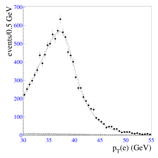
Figure 14: Transverse momentum distribution of electrons originating from the decay of a $W$ boson in hadron collisions as observed by the D0 detector at the Fermilab (Abb 00).

The measurements of the $Z$ mass at the maximum of the Breit-Wigner distribution and of the $W^{\pm}$ mass in the Jacobian peak of the lepton transverse-momentum distribution led to values in the range expected theoretically. The $W$ mass could be predicted from the Fermi coupling and the measured electroweak mixing angle $\sin^{2}\vartheta_{W}$, based on the low-energy relation (38); the $Z$ mass is directly related to the $W$ mass. Without taking into account radiative corrections, their values can be estimated as:

$$M_{W} \simeq \left[\pi\alpha\Big{/}\sqrt{2}\sin^{2}\vartheta_{W}G_{F}\right]^{1/2}\approx 79~{}{\rm GeV}$$ (87)

$$M_{Z} \simeq M_{W}\big{/}\cos\vartheta_{W}\approx 90~{}{\rm GeV}$$ (88)

Radiative corrections add shifts of about 1.5 and 1 GeV to $M_{W}$ and $M_{Z}$. The observation of the $W^{\pm}$ and $Z$ bosons in the UA1 and UA2 experiments has been an essential first step in establishing the electroweak theory of forces as a gauge theory, strongly supported moreover by the correct prediction of the $W^{\pm}$ and $Z$ masses in this framework.

3.4 High-precision electroweak scattering

In the preceding sections the Standard Model has been introduced by means of intuitive arguments. However, it can be shown that this non-Abelian gauge theory is mathematically well-defined and that observables can be calculated to an arbitrarily high precision in a systematic expansion after a few basic parameters are fixed experimentally. A series of fundamental papers (tHo 71, tHo 72) in which the Standard Model has been proven to be a renormalizable theory, played a key role in establishing the Standard Model as the basic theory of the electroweak interactions.

The high precision of the predictions on the theoretical side is matched by an equivalently high precision on the experimental side. Besides refinements of the basic scattering experiments which at early times supported the foundation of the theory, the precision achieved in $e^{+}e^{-}$ experiments at high energies, in particular at LEP and SLC, has allowed us to perform tests of the theory at the level of quantum corrections. Accuracies in general at the per-cent level, in some cases down to the per-mille level, have been achieved. The most exciting consequences of this development have been the prediction of the top quark mass which has nicely been confirmed by the direct observation at the Tevatron, and the prediction of the Higgs mass — yet to be confirmed at the time of writing.

The great potential of theoretical and experimental high-precision analyses is the sensitivity to energy scales beyond those which can be reached directly. This method may be even more important in the future when extrapolations to scales are necessary that may never be accessed by experiments directly.

3.4.1 The renormalizability of the Standard Model

In interacting field theories the emission and re-absorption of quanta after a short time of splitting, compatible with the time–energy uncertainty, alters the masses of particles and their couplings, i.e. the interactions renormalize the fundamental parameters. These effects can be described by Feynman diagrams including loops. Two characteristic examples are shown in Fig. 15.

Figure 15: Quantum corrections modifying mass and coupling parameters.

The self-energy corrections (cf. Fig. 15a) and the vertex corrections (cf. Fig. 15b) are divergent for pointlike couplings, leading to integrals of the type $\int d^{4}k/k^{4}\sim\log\Lambda_{cut}^{2}$ where $\Lambda_{cut}^{-1}$ denotes the small scale up to which the interaction appears pointlike. These contributions add to the unobservable bare mass $m_{0}$ and to the bare coupling $g_{0}$ to generate the observable physical mass $m$ and the physical coupling $g$,

$$m_{0}+\delta m = m$$

$$g_{0}+\delta g = g$$

If this renormalization prescription is sufficient to absorb all divergences and to render all other observables finite in the limit $\Lambda_{cut}^{-1}\rightarrow 0$, the theory is renormalizable and well-defined. After the masses and couplings are fixed experimentally, all other observables can be calculated, in principle to arbitrarily high precision.

Non-Abelian gauge theories, like the Standard Model, have been proven renormalizable. By fixing the electric charge $e$ and strong coupling $g_{s}$, the gauge boson masses, the fermion masses, and the Higgs mass,

$$\Re:\,e,\,g_{s},\,M_{W},\,M_{Z},\,m_{f},\,M_{H}$$

the values of all other observables can be predicted theoretically. In praxi the set $\Re$ may be replaced by the set $\Re_{exp}$,

$$\Re_{exp}:\,\alpha,\,\alpha_{s},\,G_{F},\,M_{Z},\,m_{f},\,M_{H}$$

where $\alpha=e^{2}/4\pi$ and $\alpha_{s}=g_{s}^{2}/4\pi$, to take maximal advantage of the parameters determined with the highest experimental accuracy.

The couplings $G_{F},\,\alpha$ and $\alpha_{s}$ have been determined very accurately in a long series of experiments (Cas 98).

a) The Fermi coupling $G_{F}$: The Fermi coupling is defined by the lifetime of the muon:

$$\tau^{-1}_{\mu}=\frac{G_{F}^{2}m_{\mu}^{5}}{192\pi^{3}}f\left(\frac{m_{e}^{2}}{m_{\mu}^{2}}\right)\left(1+\frac{3}{5}\frac{m_{\mu}^{2}}{M_{W}^{2}}\right)\left[1+\frac{\alpha}{2\pi}\left(\frac{25}{4}-\pi^{2}\right)+\dots\right]$$ (89)

where $f(x)=1-8x+8x^{3}-x^{4}-12x^{2}\log x$. By convention, QED corrections to the effective Fermi theory (the term in square brackets) are factored out explicitly. In the above formula we have displayed only the one-loop corrections. Other electroweak radiative corrections to the muon decay are absorbed in $G_{F}$. Including the two-loop QED corrections, one finds in the experimental analysis of the muon decay the value

$$G_{F}=1.16637(1)\times 10^{-5}\;{\rm GeV}^{-2}$$ (90)

with a relative accuracy of $10^{-5}$.

b) The Sommerfeld fine structure constant $\alpha$: The fine structure constant is generally introduced as $\alpha=e^{2}/4\pi$, defined for on-shell electrons and photons in the $ee\gamma$ vertex. Proper methods to determine this fundamental parameter are the measurements of the anomalous magnetic moment of the electron, leading to

$$\alpha^{-1}=137.03599976(50)$$

or the quantum Hall effect, with a significantly larger error though.

This definition however is not well suited for high-energy analyses. Since vacuum polarization effects screen the electric charge, the coupling increases when evaluated at a high scale of the $\gamma$ momentum transfer, $\mu_{R}=M_{Z}$ for instance: $\alpha(M_{Z}^{2})=\alpha/(1-\Delta\alpha)$.

The shift $\Delta\alpha$, induced by screening effects due to lepton and hadron loops, can be determined analytically for leptons and by a dispersion integral over the $e^{+}e^{-}$ annihilation cross section for hadrons:

$$\Delta\alpha_{lept} = \sum_{\ell=e,\mu,\tau}\frac{\alpha}{3\pi}\left(\log\frac{M_{Z}^{2}}{m_{\ell}^{2}}-\frac{5}{3}\right)+\dots$$

$$\Delta\alpha_{had} = -\frac{\alpha}{3\pi}\int\limits^{\infty}_{4m^{2}_{\pi}}\frac{M_{Z}^{2}ds^{\prime}}{s^{\prime}[s^{\prime}-M_{Z}^{2}]}\frac{\sigma(e^{+}e^{-}\rightarrow\gamma^{*}\rightarrow{\rm hadrons};s^{\prime})}{\sigma(e^{+}e^{-}\rightarrow\gamma^{*}\rightarrow\mu^{+}\mu^{-};s^{\prime})}$$ (91)

Evaluating the dispersion integral by making use of the measured annihilation cross section, the value of the coupling shifts to

$$\alpha^{-1}(M_{Z})=128.934(27)$$

This shift affects the high-precision electroweak analyses in a drastic way.

c) The strong coupling $\alpha_{s}$: Since quantum chromodynamics is an asymptotically free theory, the renormalized QCD coupling is small at high energies. Perturbative expansions can therefore be used to perform high-precision tests in processes which involve quarks and gluons. In general, the reference value of the coupling $\alpha_{s}(\mu_{R})$ is defined at the renormalization scale $\mu_{R}=M_{Z}$ in the $\overline{MS}$ scheme in which the coupling is renormalized by subtracting just the singularity in $D-4$ dimensions and a few finite constants. At the scale $M_{Z}$ five quark flavors are active in the polarization of the vacuum; they reduce the gluon-induced anti-screening of the color charge.

A large variety of experimental methods can be used at high energies to extract the QCD coupling: the cross section for $e^{+}e^{-}$ annihilation into hadrons; the hadronic decay of $\tau$ leptons; the number of jets in $Z$ decays; the hadronic event shapes; scaling violations of the structure functions; and decays of heavy quarkonia. The coupling is generally measured at scales different from $M_{Z}$. However, as long as the scales are high enough, the coupling can be evolved perturbatively to the common scale $\mu_{R}=M_{Z}$. The coupling has been determined in an overall fit as

$$\alpha_{s}(M_{Z}^{2})=0.1181\pm 0.002$$

to next-to-next-to-leading order accuracy.

3.4.2 $e^{+}e^{-}$ annihilation near the $Z$ pole

After $W^{\pm}$ and $Z$ bosons had been discovered at the Sp${\rm\bar{p}}$S, the next major step in the understanding of the $Z$ boson and the electroweak interactions have been the experiments carried out at the $e^{+}e^{-}$ storage ring LEP at CERN and the first $e^{+}e^{-}$ linear collider SLC in Stanford. At LEP about 16 million $Z$ bosons have been produced, allowing for high-statistics analyses of the electroweak interactions. SLC, on the other side, could be operated with longitudinally polarized electron and positron beams which increased the sensitivity of the electroweak measurements significantly.

The precision achieved in the LEP and SLC experiments has allowed tests of the electroweak theory at the quantum level. The experimental results have put the Glashow-Salam-Weinberg theory on very solid ground. The high-precision quantum analyses led to a tremendously successful prediction of the top-quark mass confirmed later in the Tevatron experiments, and to the prediction of a light Higgs boson, the discovery of which is eagerly awaited in the years to come. The sensitivity to quantum fluctuations in the physical observables demands the rigorous treatment of the electroweak and QCD corrections which will be described below in several consecutive steps for the basic process of fermion-pair production near the $Z$ resonance in $e^{+}e^{-}$ annihilation.

The fundamental process of fermion-pair production in $e^{+}e^{-}$ collisions,

$$e^{+}e^{-}\rightarrow f\bar{f}$$ (92)

$f$ denoting leptons and quarks, is mediated by $Z$-boson and $\gamma$ exchange in the $s$-channel, ${\cal A}={\cal A}_{Z}+{\cal A}_{\gamma}$, cf. Fig. 16 (for $f=e$, there are also $t$-channel contributions). The quantum corrections at next-to-leading order include two different components: the pure QED corrections, i.e. virtual photon corrections and real photon radiation, and the genuine electroweak corrections in loops.

Figure 16: The annihilation process $e^{+}e^{-}\to f\bar{f}$ at leading order.

a) The improved Born approximation. The basic amplitudes in lowest order, ${\cal A}^{0}_{\gamma}$ and ${\cal A}^{0}_{Z}$, are current $\times$ current amplitudes in which the electromagnetic and electroweak currents are connected by the exchange of a photon and a $Z$ boson:

$$\begin{array}[]{l}\displaystyle{\cal A}^{0}_{\gamma}=\frac{4\pi\alpha(s)Q_{e}Q_{f}}{s}j_{\mu}^{\rm em}(f)j_{\mu}^{\rm em}(e)\\[12.91663pt] \displaystyle{\cal A}^{0}_{Z}=\frac{\sqrt{2}G_{F}M_{Z}^{2}}{s-M_{Z}^{2}+iM_{Z}\Gamma_{Z}(s)}j_{\mu}^{Z}(f)j_{\mu}^{Z}(e)\end{array}$$ (93)

The coefficients $Q_{e}$, $Q_{f}$ denote the electric charges of the electron and of the fermion $f$; the electroweak currents $j_{\mu}^{Z}(e)$ and $j_{\mu}^{Z}(f)$ are coherent superpositions of a vector part proportional to $v_{e}$ and $v_{f}$, and an axial-vector part proportional to $a_{e}$ and $a_{f}$, cf. Eq. (39). By evaluating the electromagnetic coupling $\alpha(s)$ at the proper scale $s$ which characterizes the process, large logarithms from anticipated radiative corrections are incorporated in the improved Born approximation in a natural way. The Fermi coupling $G_{F}$ is related in Eq. (38) to the $SU(2)$ coupling $g_{W}$ at the scale $M_{Z}^{2}$ which is logarithmically equivalent to the proper scale $s$.

The vector and axial-vector $Z$ charges may be replaced by the partial widths $\Gamma(Z\rightarrow f\bar{f})$. The total $Z$-boson width in the Breit-Wigner denominator, interpreted as the imaginary part of the inverse $Z$ propagator at scale $s$, may be defined with an energy-dependent coefficient, $\Gamma_{Z}(s)=(s/M_{Z}^{2})\Gamma_{Z}$, while the proper $Z$ width at the pole is denoted by $\Gamma_{Z}$.

Thus, the leading logarithmic radiative corrections can easily be incorporated in the cross sections within the improved Born approximation, resulting in the cross section (Hol 00)

$$\sigma(s)=\frac{12\pi\Gamma_{e}\Gamma_{f}}{(s-M_{Z}^{2})^{2}+(s^{2}/M_{Z}^{2})\Gamma_{Z}^{2}}\left[1+\Delta_{Z}\right]+\frac{4\pi\alpha^{2}(s)}{3s}Q_{f}^{2}N_{c}$$ (94)

The first part is the Breit-Wigner form of the $Z$ contributions corrected by the real and imaginary parts

$$\Delta_{Z}=(1+R_{f})\frac{s-M_{Z}^{2}}{M_{Z}^{2}}+I_{f}\frac{\Gamma_{Z}}{M_{Z}}$$ (95)

of the $\gamma-Z$ interference contribution $R_{f}$ and $I_{f}$; the second part describes the photon-exchange contribution.

b) Electroweak corrections. The most important electroweak corrections for energies near the $Z$ resonance are self-energy corrections in the $\gamma$ and $Z$ propagators, as well as vertex corrections due to the exchange of electroweak bosons. Typical diagrams are depicted in Fig. 17. Additional box diagrams give relative corrections of less than $10^{-4}$ near the $Z$ resonance and can safely be neglected.

0.8 1

Figure 17: Typical diagrams contributing to the genuine electroweak corrections to $e^{+}e^{-}\to f\bar{f}$.

The $\rho$ parameter (Vel 77)

$$\rho_{e,f}=1+\Delta\rho+\Delta\rho_{\rm non-univ}$$ (96)

modifies the neutral-current coupling by universal corrections of the gauge boson propagators and by flavor-specific vertex corrections.

In the same way the electroweak mixing angle in the currents must be specified properly. Defining

$$\sin^{2}\vartheta_{W}=1-M_{W}^{2}/M_{Z}^{2}$$ (97)

the weak mixing angle entering in the vector $Z$ couplings of Eq. (39) are modified and replaced by effective mixing angles which are related to the basic definition as

$$\sin^{2}\vartheta^{e,f}_{\rm eff}=\kappa_{e,f}\sin^{2}\vartheta_{W}$$ (98)

Again, $\kappa_{e,f}$ can be separated into a universal and a flavor-specific part

$$\kappa_{e,f}=1+\Delta\kappa+\kappa_{\rm non-univ}$$ (99)

with

$$\Delta\kappa=\cot^{2}\vartheta_{W}\Delta\rho$$ (100)

The non-universal contribution is particularly large for the $Zbb$ coupling. After the replacement ${\cal A}_{Z}^{0}\rightarrow{\cal A}_{Z}=\sqrt{\rule{0.0pt}{7.68222pt}\rho_{e}\rho_{f}}{\cal A}_{Z}^{0}$ and $\sin^{2}\vartheta_{W}\rightarrow\sin^{2}\vartheta_{\rm eff}^{e,f}$ , the corrections $\rho_{e,f}$ and $\kappa_{e,f}$ enter the cross sections $\sigma(e^{+}e^{-}\rightarrow f\bar{f})$ and the partial widths $\Gamma(Z\rightarrow f\bar{f})$ in the same form. The expression Eq. (94) for the cross section therefore can be kept unmodified when the dominant electroweak corrections are included.

Apart from the explicit form of $\Delta\rho$ which we will give at the end of this section, we will not discuss the various corrections in detail here but instead refer the reader to the literature (Bar 99).

c) QCD corrections. These corrections affect the production cross sections for quark pairs and the partial $Z$ decay widths in the same way, when the quark masses are neglected, by the additional coefficient (Sch 73)

$$\Delta_{QCD}=1+\frac{\alpha_{s}}{\pi}+\cdots$$ (101)

Higher-order terms up to order $(\alpha_{s}/\pi)^{3}$ are known as well.

d) QED corrections. Numerically the QED corrections (Ren 81) are the most important radiative corrections near the $Z$ resonance. Since the formation of the $Z$ resonance leads to a sharp Breit-Wigner peak, the radiation of photons from the initial electrons and positrons shifts the energy $\sqrt{s}\rightarrow\sqrt{\hat{s}}$ away from the peak, resulting in a large modification of the production cross section. The cross section including the QED vertex corrections and the photon radiation in the initial state can be expressed as a convolution of the electroweak cross section $\sigma$, as calculated above, with the radiator function $H$:

$$\sigma_{QED}(s)=\int_{0}^{x_{max}}dxH(x)\sigma[(1-x)s]$$ (102)

The upper integration limit $x_{max}$ describes the maximal fraction $x$ of the photon energy not resolved in the detector. The result therefore depends strongly on possible cuts on the energies of observed photons. Without any cuts, the kinematical limit $x_{max}=2E^{\gamma}_{max}/\sqrt{s}\leq 1-4m_{f}^{2}/s$ must be inserted. Including the resummation of soft photons, the radiator function can be written in leading logarithmic order as

$$\begin{array}[]{c}H(x)=\beta x^{\beta-1}\quad{\rm with}\quad\beta=\frac{2\alpha}{\pi}\left(\log\frac{s}{m_{e}^{2}}-1\right)\end{array}$$ (103)

The complete QED corrections reduce the peak value of the resonance cross section by about $30\,\%$ and shift the position of the peak upward by about $+100$ MeV. Given the high precision of the LEP and SLC experiments, both these effects are crucial for the correct interpretation of these measurements.

Figure 18: $Z$-peak cross section observed by LEP in $e^{+}e^{-}\rightarrow hadrons$ and compared with the complete Standard Model prediction (LEP 00).

The final result for the total cross section $\sigma[e^{+}e^{-}\rightarrow hadrons]$ compared with experimental data is shown in Fig. 18 for $e^{+}e^{-}$ energies near the $Z$ resonance. After adjusting the free parameters of the electroweak theory, e.g. the $Z$-boson mass $M_{Z}$ and the electroweak mixing angle $\sin^{2}\vartheta_{W}$, the theoretical prediction of the cross section is in wonderful agreement with the data. The experimental analysis supports the validity of the Glashow-Salam-Weinberg model as the theory of the electroweak interactions at a very high level of accuracy.

Two other important observables are the forward-backward asymmetry $A_{FB}$, which describes the difference of the production cross sections for leptons and quarks in the forward and backward hemispheres with respect to the direction of the incoming electron, and the left-right asymmetry for longitudinally polarized electron and positron beams. These asymmetries can be expressed in terms of the electroweak parameters as

$$\begin{array}[]{ll}\displaystyle A_{FB}=\frac{3}{4}\frac{2v_{f}a_{f}}{v_{f}^{2}+a_{f}^{2}}\frac{2v_{e}a_{e}}{v_{e}^{2}+a_{e}^{2}}&\displaystyle\quad\Rightarrow\quad\frac{3}{4}\left[\frac{1-4\sin^{2}\vartheta_{\rm eff}^{l}}{1+(1-4\sin^{2}\vartheta_{\rm eff}^{l})^{2}}\right]^{2}\\ \displaystyle A_{LR}=\frac{2v_{e}a_{e}}{v_{e}^{2}+a_{e}^{2}}&\displaystyle\quad\Rightarrow\quad\frac{1-4\sin^{2}\vartheta_{\rm eff}^{l}}{1+(1-4\sin^{2}\vartheta_{\rm eff}^{l})^{2}}\end{array}$$ (104)

The explicit form of $A_{FB}$ as function of $\sin^{2}\vartheta_{\rm eff}^{l}$ is valid for lepton asymmetries $f=l=e$, $\mu$, $\tau$. Since for leptons $\sin^{2}\vartheta_{\rm eff}^{l}$ is near 1/4, it is apparent that the sensitivity to the value of $\sin^{2}\vartheta_{\rm eff}^{l}$ is maximal for the left-right asymmetry.

Table 2: Experimental results for several precision observables at LEP1. The pull is defined as the deviation from the theoretical prediction in units of the corresponding one-standard deviation experimental uncertainty.

Many observables have been evaluated to scrutinize the validity of the electroweak Standard Model. The measurements of a large set of observables is compared with their best values within the Standard Model in Table 2, most noticeable:

$$M_{Z}=91.1882\pm 0.0022\,{\rm GeV}$$ (105)

$$\Gamma_{Z}=2.4952\pm 0.0026\,{\rm GeV}$$ (106)

$$\sin^{2}\vartheta_{\rm eff}^{l}=0.23096\pm 0.00026$$ (107)

In several cases the agreement of the data with the predictions is at the per-mille level — a triumph of field theory as the proper formulation of electroweak interactions.

3.4.3 $W^{+}W^{-}$ gauge-boson pair production in $e^{+}e^{-}$ annihilation

The second process which could be exploited to perform precision tests of the Standard Model, is the production of $W^{\pm}$ pairs in $e^{+}e^{-}$ annihilation:

$$e^{+}e^{-}\rightarrow W^{+}W^{-}$$ (108)

This is a much cleaner production channel than for proton colliders since no additional spectator hadrons are generated in the final state. Compared with the other processes for gauge-boson pair production, $e^{+}e^{-}\rightarrow\gamma\gamma$, $\gamma Z$, $ZZ$, the process (108) constitutes the most important reaction expected to provide a detailed knowledge of the mass and the couplings of the $W$ boson.

Figure 19: $W^{+}W^{-}$ pair production in $e^{+}e^{-}$ annihilation.

The $W^{+}W^{-}$ pair production (All 77) is described by the Feynman diagrams shown in Fig. 19. Both $s$- and $t$-channel exchanges are needed in order to generate a high-energy behavior compatible with unitarity. The separate $s$- and $t$-channel contributions grow strongly with $\sqrt{s}\rightarrow\infty$ as seen in Fig. 20. The sum of all contributions which interfere destructively, leads to a reduced increase above threshold but decreases proportional to $\log(s)/s$ at large $s$. The result (All 77) valid for all $s$ reads

$$\begin{array}[]{l}\displaystyle\sigma[e^{+}e^{-}\rightarrow W^{+}W^{-}]\\[8.61108pt] \quad\displaystyle=\frac{\pi\alpha^{2}}{2s_{W}^{4}}\frac{\beta}{s}\Biggl{\{}\left[1+\frac{2M_{W}^{2}}{s}+\frac{2M_{W}^{4}}{s^{2}}\right]\frac{1}{\beta}\log\frac{1+\beta}{1-\beta}-\frac{5}{4}\\[12.91663pt] \quad\quad\displaystyle+\frac{M_{Z}^{2}(1-2s_{W}^{2})}{s-M_{Z}^{2}}\left[2\left(\frac{M_{W}^{4}}{s^{2}}+\frac{2M_{W}^{2}}{s}\right)\frac{1}{\beta}\log\frac{1+\beta}{1-\beta}-\frac{s}{12M_{W}^{2}}-\frac{5}{3}-\frac{M_{W}^{2}}{s}\right]\\[12.91663pt] \quad\quad\displaystyle+\frac{M_{Z}^{4}\left(8s_{W}^{4}-4s_{W}^{2}+1\right)\beta^{2}}{48(s-M_{Z}^{2})^{2}}\left[\frac{s^{2}}{M_{W}^{4}}+\frac{20}{M_{W}^{2}}+12\right]\Biggr{\}}\end{array}$$ (109)

with $s_{W}=\sin\vartheta_{W}$, $c_{W}=\cos\vartheta_{W}$ and $\beta=\sqrt{1-4M_{W}^{2}/s}$. The cancellation amounts to a suppression by one order of magnitude at $\sqrt{s}=400$ GeV and two orders of magnitude at $\sqrt{s}=1$ TeV, induced by the interplay of the $\gamma WW$, $ZWW$ and $e\nu W$ couplings which are related to each other by the gauge symmetry of the Standard Model.

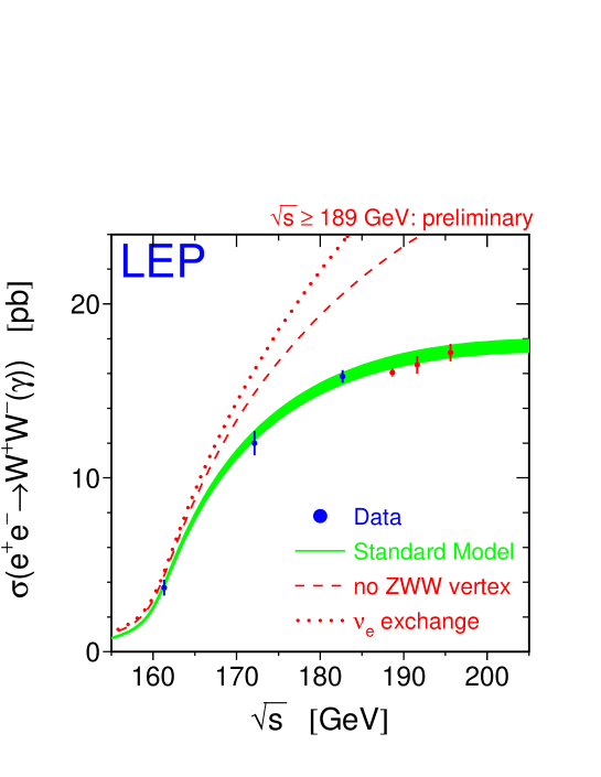
Figure 20: Total cross section for $W^{+}W^{-}$ production in $e^{+}e^{-}$ annihilation as predicted from the Standard Model (grey band), without the $s$-channel $Z$-exchange diagram (dashed line), without the $s$-channel $\gamma$, $Z$-exchange diagrams (dotted line), and compared with data from LEP2 (LEP 00a).

The measurements of the $W$-pair production cross section at LEP2 therefore provide the first determination of the 3-gauge-boson couplings $\gamma WW$ and $ZWW$. These couplings will be tested with higher accuracy at higher energies since even small anomalous couplings will upset the gauge cancellations, quickly leading to sizable deviations from the Standard Model predictions.

The detailed study of the excitation curve $\sigma_{\rm tot}(s)$ close to the threshold at $\sqrt{s}=2M_{W}$ provides a precise model-independent measurement of the $W$ mass. In terms of the velocity $\beta$, the cross section close to threshold, $\beta\ll 1$, differential in the scattering angle $\theta$, reads

$$\frac{d\sigma}{d\cos\theta}=\frac{\pi\alpha^{2}}{s}\frac{1}{2\sin^{2}\vartheta_{W}}\beta\left(1+4\beta\cos\theta\frac{3\cos^{2}\vartheta_{W}-1}{4\cos^{2}\vartheta_{W}-1}+O(\beta^{2})\right)$$ (110)

The first, $\theta$-independent term is due to the $\nu$-exchange diagram; the second term due to the two $s$-channel diagrams vanishes at threshold. As a result, the total cross section

$$\sigma_{\rm tot}=\frac{\pi\alpha^{2}}{s}\frac{1}{\sin^{2}\vartheta_{W}}\beta+O(\beta^{3})$$ (111)

rises linearly with $\beta$, and it is determined by the kinematics and the well-established $\nu eW$ coupling alone.

The dominance of the neutrino $t$-channel exchange contribution is a consequence of angular momentum and $CP$ conservation: the $s$-channel exchange of spin-1 bosons restricts the total angular momentum of the final state to $J\leq 1$. On the other hand, since at threshold $J$ is equal to the total spin of the two $W$ bosons, one can have only $J=0,$ 1, or 2. The first of these values is forbidden because of fermion-helicity conservation in the initial state, the second by $CP$ conservation. The $s$-channel contribution, as well as its interference with the $t$-channel diagram thus has to vanish at threshold.

Finite-width effects and higher-order corrections modify the above formula, but the general behavior is not altered.

Since the $W$ boson is unstable and decays into either a charged lepton and the corresponding antineutrino or into two hadron jets, the analysis of $W$-pair production requires the proper understanding of all Standard Model processes leading to four fermions in the final state $e^{+}e^{-}\rightarrow f_{1}\bar{f}_{2}f_{3}\bar{f}_{4}$. The three Feynman diagrams shown in Fig. 19 for $e^{+}e^{-}\rightarrow W^{+}W^{-}$ completed by subsequent decays of the $W$ bosons constitute only a small subset of possible Feynman diagrams for this more general process. They dominate however, if two fermions with appropriate quantum numbers have an invariant mass close to the $W$-boson mass. Investigations of the invariant mass spectrum of pairs of final state fermions therefore provide another means to measure $M_{W}$.

From the decay products of the $W^{\pm}$ bosons in the final state, $W^{\pm}\rightarrow\ell\nu,~{}~{}q\bar{q}^{\prime}$, the vector bosons can be reconstructed directly. This is a particularly useful method at energies well above the threshold in the continuum. Mixed lepton-jet pairs $\ell\nu jj$ where jets $j$ emerge as hadronization products from the original quarks, provide a very clean event sample. Four-jet final states can also be used in the analysis.

Combining all methods, from LEP as well as from the reconstruction of $W$ bosons in proton collisions, leads to the final value (LEP 00a)

$$M_{W}=80.382\pm 0.026~{}{\rm GeV}$$ (112)

for the mass of the charged $W^{\pm}$ boson.

3.4.4 Physical interpretation of the measurements

1. A most important conclusion can be drawn from the high-precision measurements of the $Z$-boson width. By observing $\Gamma_{Z}$ in the resonance excitation curve, the decay width into invisible final states of neutrino pairs can be derived by subtracting the visible charged-lepton and hadron channels with

$$\Gamma_{\rm invis} = N_{\nu}\Gamma(Z\rightarrow\nu_{\ell}\bar{\nu}_{\ell})$$ (113)

$$= N_{\nu}\frac{G_{F}M_{Z}^{3}}{12\sqrt{2}\pi}$$

the number of families in the Standard Model can be counted by measuring $N_{\nu}$, the number of light neutrinos:

$$N_{\nu}=2.994\pm 0.012$$ (114)

The measurement confirms the existence of three Standard Model families, the minimum number necessary for incorporating $CP$ violation in the theory.

2. In the canonical form of the Standard Model, the precision observables measured at the $Z$ peak are affected by quantum fluctuations; they give access to two high mass scales in the model: the top-quark mass $m_{t}$, and the Higgs-boson mass $M_{H}$. These particles enter as virtual states in the loop corrections to various relations between the electroweak observables. For instance, the radiative corrections to the relation between the $W$ and the $Z$ mass, and between the $Z$ mass and $\sin^{2}\vartheta_{\rm eff}^{l}$, have a strong quadratic dependence on $m_{t}$ and a logarithmic dependence on $M_{H}$.

More generally, quantum fluctuations from scales of physics beyond the Standard Model, e.g. supersymmetric or technicolor extensions, may also affect the electroweak observables. The modifications can either be exploited to scrutinize hypothetical extensions or, at least, to constrain the new scales characterizing the extended theories.

A second area of new physics phenomena are possible deviations of the interactions between the electroweak gauge bosons from the predictions of the Standard Model. The form and the strength of the trilinear couplings are predicted by the non-Abelian gauge symmetry. They can be measured in the production of $W^{+}W^{-}$ pairs in $e^{+}e^{-}$ annihilation. These experiments therefore serve to verify one of the most important symmetry concepts in Nature.

a) The masses of the top quark and the Higgs boson. Eliminating either $M_{W}$ or $\sin^{2}\vartheta_{W}$ from the basic low-energy connection between the Fermi constant, the $W$ mass and the electroweak mixing angle, the connection may be written in two forms. In the first case,

$$\sin^{2}\vartheta_{\rm eff}^{\ell}\left(1-\sin^{2}\vartheta_{\rm eff}^{\ell}\right)=\frac{\pi\alpha}{\sqrt{2}G_{F}M_{Z}^{2}\left(1-\Delta r_{Z}\right)}$$ (115)

The correction $\Delta r_{Z}$ includes the shift $\alpha\rightarrow\alpha(M_{Z}^{2})$ and the contribution from top-bottom and Higgs fluctuations in the propagators of the electroweak vector bosons, cf. Fig. 21,

Figure 21: Top-bottom and Higgs-boson loops contributing to the $W$ boson self-energy.

$$\Delta r_{Z}=\Delta\alpha-\Delta\rho^{t}+\Delta r_{Z}^{H}+\cdots$$ (116)

The shift $\Delta\alpha$ of the electromagnetic coupling has been discussed earlier. The leading top contribution to the $\rho$ parameter (Vel 77) is quadratic in $m_{t}$:

$$\Delta\rho^{t}=\frac{3G_{F}m_{t}^{2}}{8\pi^{2}\sqrt{2}}+\cdots$$ (117)

The Higgs contribution is screened, depending only logarithmically on the Higgs-boson mass for large $M_{H}$:

$$\Delta r_{Z}^{H}=\frac{G_{F}M_{W}^{2}}{8\pi^{2}\sqrt{2}}\frac{1+9\sin^{2}\vartheta_{W}}{3\cos^{2}\vartheta_{W}}\log\frac{M_{H}^{2}}{M_{W}^{2}}+\cdots$$ (118)

Alternatively, the relation can be written in terms of $M_{W}$:

$$\frac{M_{W}^{2}}{M_{Z}^{2}}\left(1-\frac{M_{W}^{2}}{M_{Z}^{2}}\right)=\frac{\pi\alpha}{\sqrt{2}G_{F}M_{Z}^{2}\left(1-\Delta r_{W}\right)}$$ (119)

where the quantum correction $\Delta r_{W}$ is composed of

$$\Delta r_{W}=\Delta\alpha-\cot^{2}\vartheta_{W}\Delta\rho^{t}+\Delta r_{W}^{H}+\cdots$$ (120)

with

$$\Delta r_{W}^{H}=\frac{G_{F}M_{W}^{2}}{8\pi^{2}\sqrt{2}}\frac{11}{3}\log\frac{M_{H}^{2}}{M_{W}^{2}}+\cdots$$ (121)

and $\Delta\alpha$ and $\Delta\rho^{t}$ as introduced above.

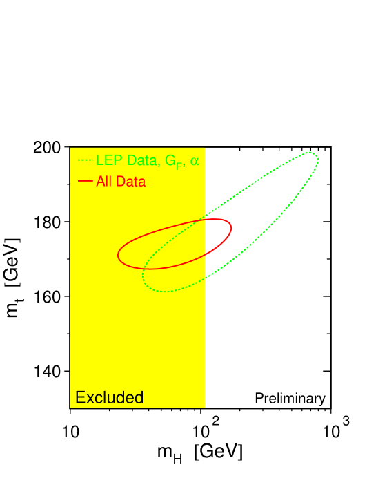
Figure 22: Allowed region in the $m_{t}-M_{H}$ plane derived from a fit of LEP results to the Standard Model predictions (LEP 00a).

Inserting the precision data for $\alpha$, $G_{F}$, $M_{Z}$ and $\sin^{2}\vartheta_{\rm eff}^{l}$ in the first case or $M_{W}$ in the second case, these relations can be solved for $m_{t}$ and $M_{H}$. The final results for all the precision observables have been used to determine the top and the Higgs-boson masses as demonstrated in Fig. 22. The value of the top mass obtained from the global fit (LEP 00a)

$${\it indirect~{}precision~{}measurements:~{}~{}}m_{t}=169.7^{+9.8}_{-7.0}~{}{\rm GeV}$$ (122)

is in excellent agreement with the value measured directly in top-quark production at the Tevatron (Abb 98, Yao 98):

$${\it direct~{}experimental~{}measurements:~{}~{}}m_{t}=174.3\pm 5.1~{}{\rm GeV}$$ (123)

In fact, the prediction of $m_{t}$ from the electroweak precision analyses was in agreement with the directly measured value within 15 GeV.

The correctly predicted value of the top-quark mass raises hope that the second prediction may also be realized in Nature. Fixing the top mass to the experimental value, the evaluation of the precision data leads to the following values for the Higgs-boson mass (LEP 00a):

$$\begin{array}[]{l}M_{H}=77^{+69}_{-39}~{}{\rm GeV}\\ M_{H}<215~{}{\rm GeV~{}~{}at}~{}~{}95\,\%{\rm CL}\end{array}$$ (124)

Due to yet unknown two-loop corrections, the accuracy of the analysis is expected in the range of 100 GeV. This prediction is exciting for several reasons: (i) The numbers are compatible with a light Higgs-boson mass in the characteristic range of the scales of the electroweak symmetry breaking between $M_{W}\simeq 81$ GeV and $v/\sqrt{2}\simeq 174$ GeV; (ii) The small Higgs-boson mass is a prerequisite for extending the Standard Model to grand unification scales; in this way the value of the electroweak mixing angle is predicted correctly in the range observed experimentally. Moreover, the restricted mass range of the Higgs boson is nicely compatible with the low mass value expected in supersymmetric theories which are attractive extensions of the Standard Model.

b) $S$, $T$, $U$ parameters. Generalizing the previous analysis, a special class of “new physics” contributions can be described by the $S$, $T$, $U$ parameters (Pes 90). They account for the quantum fluctuations of the electroweak bosons into new heavy states which have negligible couplings to the light leptons and quarks. Expanding the self energies of the electroweak bosons generated by the new physics contributions, about $Q^{2}=0$,

$$\begin{array}[]{ll}\displaystyle\Pi_{\gamma\gamma}(Q^{2})=Q^{2}\Pi^{\prime}_{\gamma\gamma}(0)+\cdots\,,&\displaystyle\Pi_{ZZ}(Q^{2})=\Pi_{ZZ}(0)+Q^{2}\Pi^{\prime}_{ZZ}(0)+\cdots\\ \displaystyle\Pi_{\gamma Z}(Q^{2})=Q^{2}\Pi^{\prime}_{\gamma Z}(0)+\cdots\,,&\displaystyle\Pi_{WW}(Q^{2})=\Pi_{WW}(0)+Q^{2}\Pi^{\prime}_{WW}(0)+\cdots\end{array}$$ (125)

three of the six parameters are absorbed in the renormalized input parameters $\alpha$, $G_{F}$ and $M_{Z}$, whereas the other three are new observables:

$$\begin{array}[]{l}\displaystyle S=\frac{\sin^{2}2\vartheta_{W}}{\alpha}\left(\Pi^{\prime}_{ZZ}(0)-2\cot 2\vartheta_{W}\Pi^{\prime}_{Z\gamma}(0)-\Pi^{\prime}_{\gamma\gamma}(0)\right)\\[12.91663pt] \displaystyle T=\frac{1}{\alpha}\left(\frac{\Pi_{WW}(0)}{M_{W}^{2}}-\frac{\Pi_{ZZ}(0)}{M_{Z}^{2}}\right)\\[12.91663pt] \displaystyle U=\frac{4\sin^{2}\vartheta_{W}}{\alpha}\left(\Pi^{\prime}_{WW}(0)-\cos^{2}\vartheta_{W}\Pi^{\prime}_{ZZ}(0)-\sin 2\vartheta_{W}\Pi^{\prime}_{Z\gamma}(0)-\sin^{2}\vartheta_{W}\Pi^{\prime}_{\gamma\gamma}(0)\right)\end{array}$$ (126)

The parameters have been determined in a global fit to the electroweak precision data. After subtracting the contributions from the Standard Model at $M_{H}=M_{Z}$, the result (Cas 98) is

$$\begin{array}[]{l}S=-0.16\pm 0.14\\ T=-0.21\pm 0.16\\ U=+0.25\pm 0.24\end{array}$$ (127)

The parameter $T$ corresponds to $\Delta\rho$ and measures the weak isospin breaking, and so does $U$. In fact, the contributions of any new isodoublet with masses $m_{U}$ and $m_{D}$ to the three parameters are given by

$$\begin{array}[]{l}\displaystyle S=\frac{1}{6\pi}\left(1-Y\log\frac{m_{U}^{2}}{m_{D}^{2}}\right)\\[12.91663pt] \displaystyle T=\frac{1}{4\pi\sin^{2}2\vartheta_{W}M_{Z}^{2}}\left(m_{U}^{2}+m_{D}^{2}-\frac{2m_{U}^{2}m_{D}^{2}}{m_{U}^{2}-m_{D}^{2}}\log\frac{m_{U}^{2}}{m_{D}^{2}}\right)\\[12.91663pt] \displaystyle U=\frac{1}{6\pi}\left(-\frac{5m_{U}^{4}-22m_{U}^{2}m_{D}^{2}+5m_{D}^{4}}{3(m_{U}^{2}-m_{D}^{2})^{2}}+\frac{m_{U}^{6}-3m_{U}^{4}m_{D}^{2}-3m_{U}^{2}m_{D}^{4}+m_{D}^{6}}{(m_{U}^{2}-m_{D}^{2})^{3}}\log\frac{m_{U}^{2}}{m_{D}^{2}}\right)\\ \end{array}$$ (128)

where $Y$ represents the hypercharge of the doublet. Since $T$ is measured to be very small, the new up and down masses must be nearly degenerate. In this limit, the expressions simplify:

$$\begin{array}[]{l}\displaystyle S=\frac{1}{6\pi}\simeq 0.05\\[8.61108pt] \displaystyle T=\frac{1}{3\pi\sin^{2}2\vartheta_{W}}\frac{(m_{U}-m_{D})^{2}}{M_{Z}^{2}}\\[8.61108pt] \displaystyle U=\frac{2}{15\pi}\frac{(m_{U}-m_{D})^{2}}{m_{U}^{2}}\end{array}$$ (129)

While the contributions to $T$ and $U$ are suppressed for nearly degenerate isodoublet masses, this is different for $S$; for a multiplet of heavy degenerate chiral fermions:

$$S=\frac{N_{c}}{3\pi}\sum_{i}\left(I_{3L}^{i}-I_{3R}^{i}\right)^{2}$$ (130)

A very important application of these measurements scrutinizes technicolor theories of electroweak symmetry breaking. In these approaches the doublets add up to a value as large as $S\simeq 1.6$ if they are formulated as QCD-type theories, in disagreement with the experimentally observed value for $S$. This discrepancy can be avoided only if the non-perturbative dynamics is extended to high scales as formulated in walking-technicolor scenarios.

Supersymmetric theories however pass this control gate in a natural way: Since the new degrees of freedom decouple for asymptotic values of the masses, the contribution to the $S$, $T$, $U$ parameters can be reduced to negligible size.

c) $W$ interactions and non-Abelian gauge symmetry. The non-Abelian gauge symmetry $SU(2)\times U(1)$ of the electroweak interactions predicts the form and the strength of the trilinear $\gamma W^{+}W^{-}$ and $ZW^{+}W^{-}$ vertices. In the most general scenarios these couplings are described each by seven parameters (Gae 79). Assuming $C$, $P$ and $T$ invariance in the pure electroweak boson sector, the number of static parameters is reduced to three,

$${\cal L}_{k}/ig_{k}=g^{1}_{k}W^{\ast}_{\mu\nu}W_{\mu}A_{\nu}^{k}+\kappa_{k}W^{\ast}_{\mu}W_{\nu}F_{\mu\nu}^{k}+\frac{\lambda_{k}}{M_{W}^{2}}W^{\ast}_{\rho\mu}W_{\mu\nu}F_{\nu\rho}^{k}$$ (131)

for $k=\gamma$, $Z$ with $g_{\gamma}=e$ and $g_{Z}=e\cot\vartheta_{W}$. The parameters $g_{\gamma}^{1}=1$, $g_{Z}^{1}=1+\Delta g_{Z}^{1}$, $\kappa_{k}=1+\Delta\kappa_{k}$ and $\lambda_{k}$ can be identified with the $\gamma$ and $Z$ charges of the $W$ bosons and the related magnetic dipole moments $\mu_{k}$ and electric quadrupole moments $Q_{k}$:

$$\begin{array}[]{rl}\displaystyle\mu_{\gamma}=\frac{e}{2M_{W}}\left[2+\Delta\kappa_{\gamma}+\lambda_{\gamma}\right]&\quad\displaystyle\mu_{Z}=\frac{e\cot\vartheta_{W}}{2M_{W}}\left[2+\Delta g_{Z}^{1}+\Delta\kappa_{Z}+\lambda_{Z}\right]\\[8.61108pt] \displaystyle Q_{\gamma}=-\frac{e}{M_{W}^{2}}\left[1+\Delta\kappa_{\gamma}-\lambda_{\gamma}\right]&\quad\displaystyle Q_{Z}=-\frac{e}{M_{W}^{2}}\left[1+\Delta\kappa_{Z}-\lambda_{Z}\right]\end{array}$$ (132)

The gauge symmetries of the Standard Model demand $g_{k}^{1}=1$, $\kappa_{k}=1$ and $\lambda_{k}=0$. The magnetic dipole and the electric quadrupole moments can be measured directly in the production of $W\gamma$ and $WZ$ pairs at $p\bar{p}$ and $pp$ colliders and $WW$ pairs at $e^{+}e^{-}$ and $\gamma\gamma$ colliders.

Detailed experimental analyses have been carried out for the reaction $e^{+}e^{-}\rightarrow W^{+}W^{-}\rightarrow(l\nu_{l})(q\bar{q}^{\prime})$. Presently the bounds from LEP2 are of the order of a few percent, those from the Tevatron slightly larger. Bounds on $\Delta\kappa$ and $\lambda$ which are expected at $e^{+}e^{-}$ colliders (Zer 99) at $\sqrt{s}=500$ GeV,

$$\begin{array}[]{rl}&\quad\Delta g_{Z}^{1}=2.5\times 10^{-3}\\ \Delta\kappa_{\gamma}=4.8\times 10^{-4}&\quad\Delta\kappa_{Z}=7.9\times 10^{-4}\\ \lambda_{\gamma}=7.2\times 10^{-4}&\quad\lambda_{Z}=6.5\times 10^{-4}\end{array}$$ (133)

are significantly better than the bounds expected from the LHC. High-precision tests can therefore be performed in the near future on one of the most basic symmetries of the electroweak interactions.

3.5 Dynamics of the Higgs sector

The Higgs sector (Hig 64, Eng 64, Gur 64) is the cornerstone for the consistent field-theoretic description of the electroweak interactions which include non-zero masses for the gauge bosons. The Higgs mechanism manifests itself in the existence of a spin-zero particle, the Higgs-boson, the properties of which have been discussed earlier. The discovery of the Higgs-particle is the experimentum crucis of the Standard Model. The most important scattering processes in which this particle can be searched for will therefore be summarized briefly.

A surplus of events has recently been observed in LEP experiments (Acc 00, Bar 00) in the 4-jet channel and in the channel 2-jet $+$ missing energy when the machine was operated at the highest possible energy above 206 GeV. Since clearly identified $b$ quarks have been isolated in the jets, these events are compatible with the expected Higgs signal for $M_{H}=115.0{}^{+1.3}_{-0.9}$ GeV. However, with $2.9\,\sigma$, the rejection of the surplus as a possible statistical fluctuation or the increase of the significance are reserved for future experiments.

3.5.1 Higgs production channels at $e^{+}e^{-}$ colliders

The main production mechanisms (Spi 97) for Higgs bosons in $e^{+}e^{-}$ collisions are

Higgs-strahlung $$e^{+}e^{-}\to Z^{*}\to ZH$$ (134)

$$WW e^{+}e^{-}\to\bar{\nu}_{e}\nu_{e}(WW)\to\bar{\nu}_{e}\nu_{e}H$$ fusion (135)

In the Higgs-strahlung process the Higgs boson is emitted from the $Z$-boson line, while $WW$ fusion is a formation process of Higgs bosons in the collision of two quasi-real $W$ bosons radiated off the electron and positron beams.

In the LEP2 experiments, the SM Higgs has been searched for, unsuccessfully, in the mass range up to about 112 GeV. The high-energy $e^{+}e^{-}$ linear colliders can cover the entire Higgs mass range in the second phase of the machines in which they will reach a total energy of about 2 TeV.

a) Higgs-strahlung. The cross section for Higgs-strahlung can be written in a compact form as

$$\sigma(e^{+}e^{-}\to ZH)=\frac{G_{F}^{2}M_{Z}^{4}}{96\pi s}\left[v_{e}^{2}+a_{e}^{2}\right]\lambda^{1/2}\frac{\lambda+12M_{Z}^{2}/s}{\left[1-M_{Z}^{2}/s\right]^{2}}$$ (136)

where $v_{e}$ and $a_{e}$ were defined in Eq. (39) and $\lambda=[1-(M_{H}+M_{Z})^{2}/s][1-(M_{H}-M_{Z})^{2}/s]$ is the usual two-particle phase-space function. The cross section is of the size $\sigma\sim g_{W}^{4}/s$, i.e. of second order in the weak coupling, and it scales in the squared energy.

Figure 23: The cross section for the production of SM Higgs bosons in Higgs-strahlung $e^{+}e^{-}\to ZH$ and $WW/ZZ$ fusion $e^{+}e^{-}\to\bar{\nu}_{e}\nu_{e}/e^{+}e^{-}H$; solid curves: $\sqrt{s}=500$ GeV, dashed curves: $\sqrt{s}=800$ GeV; (Spi 97).

Since the cross section vanishes for asymptotic energies, the Higgs-strahlung process is most useful for the search for Higgs bosons in the range where the collider energy is of the same order as the Higgs mass, $\sqrt{s}{\raisebox{-3.69899pt}{~{}\shortstack{$>$ \\ [-0.07cm] $\sim$}}~{}}{\cal O}(M_{H})$. The size of the cross section is illustrated in Fig. 23 for an $e^{+}e^{-}$ linear collider with the energy $\sqrt{s}=500$ GeV as a function of the Higgs mass. Since the recoiling $Z$ in the two-body reaction $e^{+}e^{-}\to ZH$ is mono-energetic, the mass of the Higgs boson can be reconstructed from the energy of the $Z$ boson, $M_{H}^{2}=s-2\sqrt{s}E_{Z}+M_{Z}^{2}$, without any need to analyze the decay products of the Higgs boson. For leptonic $Z$ decays, missing-mass techniques provide a very clear signal.

b) $WW$ fusion. Also the cross section for the fusion process (135) can be cast implicitly into a compact form:

$$\sigma(e^{+}e^{-}\to\bar{\nu}_{e}\nu_{e}H) = \frac{G_{F}^{3}M_{W}^{4}}{4\sqrt{2}\pi^{3}}\int_{\kappa_{H}}^{1}dx\int_{x}^{1}dy\frac{1}{[1+(y-x)/\kappa_{W}]^{2}}f(x,y)$$ (137)

$$f(x,y) = \left(\frac{2x}{y^{3}}-\frac{1+3x}{y^{2}}+\frac{2+x}{y}-1\right)\left[\frac{z}{1+z}-\log(1+z)\right]+\frac{x}{y^{3}}\frac{z^{2}(1-y)}{1+z}$$

with $\kappa_{H,W}=M_{H,W}^{2}/s$ and $z=y(x-\kappa_{H})/(\kappa_{W}x)$.

Since the fusion process is a $t$-channel exchange process, the size is set by the Compton wavelength of the $W$, suppressed however with respect to Higgs-strahlung by the third order of the electroweak coupling, $\sigma\sim g_{W}^{6}/M_{W}^{2}$. As a result, $WW$ fusion becomes the leading production process for Higgs particles at high energies. At asymptotic energies the cross section simplifies to

$$\sigma(e^{+}e^{-}\to\bar{\nu}_{e}\nu_{e}H)\to\frac{G_{F}^{3}M_{W}^{4}}{4\sqrt{2}\pi^{3}}\left[\log\frac{s}{M_{H}^{2}}-2\right]$$ (138)

In this limit, $WW$ fusion to Higgs bosons can be interpreted as a two-step process: the $W$ bosons are radiated as quasi-real particles from electrons and positrons, $e\to\nu W$, with the Higgs bosons formed subsequently in the colliding $W$ beams.

The size of the fusion cross section is compared with Higgs-strahlung in Fig. 23. At $\sqrt{s}=500$ GeV the two cross sections are of the same order, yet the fusion process becomes increasingly important with rising energy.

c) $\gamma\gamma$ fusion. The production of Higgs bosons in $\gamma\gamma$ collisions can be exploited to determine important properties of these particles, in particular the two-photon decay width. The $H\gamma\gamma$ coupling is mediated by loops of charged particles. If the mass of the loop particle is generated through the Higgs mechanism, the decoupling of the heavy particles is lifted and the $\gamma\gamma$ width reflects the spectrum of these states with masses possibly far above the Higgs mass.

The two-photon width is related to the production cross section for polarized $\gamma$ beams by

$$\sigma(\gamma\gamma\to H)=\frac{16\pi^{2}\Gamma(H\to\gamma\gamma)}{M_{H}}\times BW(s_{\gamma\gamma}-M_{H}^{2})$$ (139)

where $BW$ denotes the Breit-Wigner resonance factor as a function of the $\gamma\gamma$ energy. For narrow Higgs bosons the observed cross section is found by folding the $\gamma\gamma$ cross section with the invariant $\gamma\gamma$ energy flux $\tau d{\cal L}^{\gamma\gamma}/d\tau$ at $\tau=M_{H}^{2}/s_{ee}$.

The event rate for the production of Higgs bosons in $\gamma\gamma$ collisions of Weizsäcker-Williams photons is too small to play a role in practice. However, the rate is sufficiently large if the photon spectra are generated by Compton back-scattering of laser light. The $\gamma\gamma$ invariant energy in such a Compton collider is nearly of the same size as the parent $e^{+}e^{-}$ energy and the luminosity is expected to be only slightly smaller than the luminosity in $e^{+}e^{-}$ collisions. In the Higgs mass range between 100 and 150 GeV, the final state consists primarily of $b\bar{b}$ pairs. The large $\gamma\gamma$ continuum background is suppressed in the $J_{z}^{\gamma\gamma}=0$ polarization state. For Higgs masses above 150 GeV, $WW$ final states become dominant, supplemented by $ZZ$ final states above the $ZZ$ decay threshold in the ratio 1:2. While the continuum $WW$ background in $\gamma\gamma$ collisions is very large, the $ZZ$ background appears controllable for masses up to order 300 GeV.

3.5.2 Higgs production at hadron colliders

Several processes can be exploited to produce Higgs particles in hadron colliders (Spi 97):

	gluon fusion	$gg\to H$
	$WW,ZZ$ fusion	$W^{+}W^{-},ZZ\to H$
	Higgs-strahlung off $W,Z$	$q\bar{q}\to W,Z\to W,Z+H$
	Higgs bremsstrahlung off top	$q\bar{q},gg\to t\bar{t}+H$

While gluon fusion plays a dominant role throughout the entire Higgs mass range of the Standard Model, the $WW$ and $ZZ$ fusion processes become increasingly important with rising Higgs mass. The last two radiation processes are relevant only for light Higgs masses.

The production cross sections at hadron colliders, at the LHC in particular, are quite sizeable so that a large sample of SM Higgs particles can be produced in this machine. Experimental difficulties arise from the huge number of background events that come along with the Higgs signal events. This problem will be tackled by either triggering on leptonic decays of $W,Z$ and $t$ in the radiation processes or by exploiting the resonance character of the Higgs decays $H\to\gamma\gamma$ and $H\to ZZ\to 4\ell^{\pm}$. In this way, the Tevatron is expected to search for Higgs particles in the mass range above that of LEP2, extended to $\sim 180$ GeV only for high-luminosity operation. The LHC is expected to cover the entire canonical Higgs mass range $M_{H}{\raisebox{-3.69899pt}{~{}\shortstack{$<$ \\ [-0.07cm] $\sim$}}}~{}700$ GeV of the Standard Model (ATL 99, CMS 94).

a) Gluon fusion. The gluon-fusion mechanism

$$pp\to gg\to H$$

provides the dominant production mechanism of Higgs bosons at the LHC in the entire relevant Higgs mass range up to about 1 TeV. The gluon coupling to the Higgs boson in the SM is mediated by triangular loops of top and bottom quarks as shown in Fig. 24. Since the Yukawa coupling of the Higgs particle to heavy quarks grows with the quark mass, thus balancing the decrease of the amplitude, the form factor approaches a non-zero value for infinitely heavy quarks in the loop. If the masses of heavy quarks beyond the third generation were generated solely by the Higgs mechanism, these particles would add the same amount to the form factor as the top quark in the asymptotic heavy-quark limit.

Figure 24: The formation of Higgs bosons in gluon-gluon collisions.

The partonic cross section, Fig. 24, can be expressed by the gluonic width of the Higgs boson at lowest order:

$$\hat{\sigma}_{LO}(gg\to H)=\frac{\pi^{2}}{8}\frac{\Gamma(H\to gg)}{M_{H}}\times BW(\hat{s}-M_{H}^{2})$$ (140)

where $\hat{s}$ denotes the partonic cms-energy squared. In the narrow-width approximation, the hadronic cross section can be cast into the form

$$\sigma_{LO}(pp\to H)=\frac{\pi^{2}}{8s}\frac{\Gamma(H\to gg)}{M_{H}}\frac{d{\cal L}^{gg}}{d\tau}$$ (141)

with $d{\cal L}^{gg}/d\tau$ denoting the $gg$ luminosity of the $pp$ collider, evaluated for the Drell-Yan variable $\tau=M_{H}^{2}/s$, where $s$ is the total hadronic energy squared.

The size of the radiative QCD corrections can be parametrized by defining the $K$ factor as $K=\sigma_{NLO}/\sigma_{LO}$. The virtual corrections $K_{virt}$ and the real corrections $K_{gg}$ for the $gg$ collisions are of the same size, and both are large and positive; the corrections for $q\bar{q}$ collisions and the $gq$ inelastic Compton contributions are less important. After including these higher-order QCD corrections, the theoretical uncertainty in the prediction of the cross section is significantly reduced from a level of ${\cal O}(100\%)$ down to a level of about 20%.

The theoretical prediction for the production cross section of Higgs particles is presented in Fig. 25 for the LHC as a function of the Higgs mass. The cross section decreases with increasing Higgs mass. This is, to a large extent, a consequence of the sharply falling $gg$ luminosity for large invariant masses. The bump in the cross section is induced by the $t\bar{t}$ threshold in the top triangle. The overall theoretical accuracy of this calculation is expected to be at a level of 20 to 30%.

b) Vector-boson fusion. The second important channel for Higgs production at the LHC is vector-boson fusion, $W^{+}W^{-}\to H$. For large Higgs masses this mechanism becomes competitive with gluon fusion; for intermediate masses the cross section is smaller by about an order of magnitude.

For large Higgs masses, the two electroweak bosons $W$, $Z$ which form the Higgs boson, are predominantly polarized longitudinally. At high energies, the equivalent particle spectra of the longitudinal $W$, $Z$ bosons in quark beams are given by

$$f^{W}_{L}(x) = \frac{G_{F}M_{W}^{2}}{2\sqrt{2}\pi^{2}}\frac{1-x}{x}$$ (142)

$$f^{Z}_{L}(x) = \frac{G_{F}M_{Z}^{2}}{8\sqrt{2}\pi^{2}}\left[v_{q}^{2}+a_{q}^{2}\right]\frac{1-x}{x}$$

where $x$ is the fraction of energy transferred from the quark to the $W$, $Z$ boson in the splitting process $q\to q+W/Z$. Denoting the parton cross section for $WW,ZZ\to H$ by $\hat{\sigma}_{0}$ with

$$\hat{\sigma}_{0}(VV\to H)=\sqrt{2}\pi G_{F}\delta\left(1-M_{H}^{2}/M_{VV}^{2}\right)$$ (143)

the cross section for Higgs production in quark-quark collisions is given by

$$\hat{\sigma}(qq\to qqH)=\sqrt{2}\pi G_{F}\frac{d{\cal L}^{VV}}{d\tau_{VV}}$$ (144)

with $\tau_{VV}=M_{VV}^{2}/\hat{s}$. The hadronic cross section is finally obtained by summing the parton cross section (144) over the flux of all possible pairs of quark-quark and antiquark combinations:

$$\sigma(qq^{\prime}\to VV\to H)=\int_{M_{H}^{2}/s}^{1}d\tau\sum_{qq^{\prime}}\frac{d{\cal L}^{qq^{\prime}}}{d\tau}\hat{\sigma}(qq^{\prime}\to qq^{\prime}H;\hat{s}=\tau s)$$ (145)

Since to lowest order the proton remnants are color singlets in the $WW$, $ZZ$ fusion processes, no color will be exchanged, at next-to-leading order, between the two quark lines from which the two vector bosons are radiated. As a result, the leading QCD corrections to these processes are already accounted for by the corrections to the quark parton densities.

The sum of the $WW$ and $ZZ$ fusion cross sections for Higgs bosons at the LHC is shown in Fig. 25. The process is apparently most important in the upper range of Higgs masses, where the cross section approaches values close to gluon fusion.

c) Higgs-strahlung off vector bosons. Higgs-strahlung $q\bar{q}\to V^{*}\to VH~{}(V=W,Z)$ is a very important mechanism (cf. Fig. 25) for the search of light Higgs bosons at the hadron colliders Tevatron and LHC. Though the cross section is smaller than for gluon fusion, leptonic decays of the electroweak vector bosons are extremely useful to filter Higgs signal events out of the huge background. Since the dynamical mechanism is the same as for $e^{+}e^{-}$ colliders, except for the folding with the quark-antiquark densities, intermediate steps of the calculation need not be noted in detail, and the final values of the cross sections for the Tevatron and the LHC are recorded in Fig. 25.

d) Higgs bremsstrahlung off top quarks. Also the processes $gg,q\bar{q}\to t\bar{t}H$ are relevant only for small Higgs-boson masses (cf. Fig. 25). The analytical expression for the parton cross section, even at lowest order, is quite involved, so that just the final results for the LHC cross section are shown in Fig. 25.

Higgs bremsstrahlung off top quarks is an interesting process for measurements of the $Htt$ Yukawa coupling. The cross section $\sigma(pp\to t\bar{t}H)$ is directly proportional to the square of this fundamental coupling.

Figure 25: Higgs-production cross sections at the LHC for various production mechanisms as a function of the Higgs mass. QCD corrections are included except for Higgs bremsstrahlung; cf. (Spi 97).

Summary. An overview of the production cross sections for Higgs particles at the LHC is presented in Fig. 25. Three classes of channels can be distinguished. The gluon fusion of Higgs particles is a universal process, dominant over the entire SM Higgs mass range. Higgs-strahlung off electroweak $W$ and $Z$ bosons or top quarks is prominent for light Higgs bosons. The $WW$ and $ZZ$ fusion channels, by contrast, become increasingly important for large values of the SM Higgs boson.

The signatures for the search of Higgs particles are dictated by the decay branching ratios. In the lower part of the intermediate mass range between 100 and 180 GeV, resonance reconstruction in $\gamma\gamma$ final states and $b\bar{b}$ jets can be exploited. In the upper part of the intermediate mass range, decays to pairs of virtual and real $ZZ$ and $WW$ bosons are important, with the two electroweak bosons decaying leptonically. In the mass range above the on-shell $ZZ$ decay threshold, the charged-lepton decays $H\to ZZ\to 4\ell^{\pm}$ provide gold-plated signatures. At the upper end of the classical Standard Model Higgs-mass range, decays to neutrinos and jets, generated in $W$ and $Z$ decays, complete the search techniques.

4 Summary and Perspectives

Ingenious theoretical and experimental developments have led to a clear picture of the structure of Nature, formulated at microscopic distances. The Standard Model of particle physics is based on quantum field theory. The fundamental constituents of matter are leptons and quarks. Abelian and non-Abelian gauge symmetries are the platform on which the electroweak and strong forces are built up. The particle masses are generated by interactions with a scalar field.

A large variety of experiments in hadron-hadron scattering, lepton-nucleon scattering and electron-positron annihilation have established essential elements of this picture in the past decades. The ensemble of three lepton-quark families has been completed. The $SU(3)\times SU(2)\times U(1)$ gauge symmetry has been established in the interactions of leptons and quarks with the gauge fields, partly with accuracies at the per-mille level. The same level of experimental accuracy can be envisaged for the interactions among the gauge bosons when the future proton-proton collider LHC and prospective electron-positron linear colliders will operate in the TeV energy range. The most pressing experimental problem within the Standard Model however appears to be the Higgs mechanism which has been introduced to generate the masses of the fundamental particles in a way consistent with the gauge symmetries. The production processes for the Higgs particle at the LHC will cover the entire canonical mass range of the Standard Model in the near future and $e^{+}e^{-}$ colliders can scrutinize the dynamics of the Higgs mechanism.

Even though the Standard Model provides a valid frame for physics from microscopic to macroscopic scales, the model cannot be considered as ultima ratio of Nature. (i) The separate electro–weak and strong gauge symmetries should be unified in a simple group. Attempts to unify $SU(3)\times SU(2)\times U(1)$ in $SU(5)$ at scales of order $10^{16}$ GeV predict the electroweak mixing angle approximately in the correct range $\sin^{2}\vartheta_{W}\sim 0.2$. This signals a step in the right direction even though the picture must be considered oversimplified for many reasons. Embedding the Standard Model at the TeV scale in a supersymmetric theory in which fermionic and bosonic degrees of freedom are unified, offers a solution for many of the conceptual problems. The coexistence of vastly different scales, the Planck scale at $M_{\rm Pl}\sim 10^{19}$ GeV and the electroweak scale $v/\sqrt{2}\sim 174$ GeV, is stabilized by this theory and the proton decay can be suppressed. (ii) Gravity is attached ad hoc to the Standard Model and not incorporated properly in the theory. Again, supersymmetry formulated as a local symmetry provides a first raison d’être for the spin-2 gravitational field. (iii) A consistent quantum theory of gravity may break the frame of local field theory. Theories of extended superstrings offer the solution of this problem. Moreover, they unify gravity with particle physics. This approach should provide answers to many problems of the Standard Model: the symmetry structure; the family structure; the prediction of the large number of mass parameters and couplings. Such a theory to which the Standard Model would be an essential element, could describe Nature between the Planck length of $10^{-33}$ cm and the scale $10^{+28}$ cm of the Universe.

Future scattering experiments at TeV energies will be crucial for establishing such a comprehensive theory of matter and forces.

5 References

Abachi S et al (1995) (D0 Collaboration) Phys. Rev. Lett. 74 2632

Abbott B et al (1998) (D0 Collaboration) Phys. Rev. D58 052001

Abbott B et al (2000) (D0 Collaboration) Phys. Rev. D62 092006

Abe F et al (1995) (CDF Collaboration) Phys. Rev. Lett. 74 2626

Abe F et al (1999) (CDF Collaboration) Phys. Rev. D59 052002

Acciari M et al (2000) (L3 Collaboration) Report CERN-EP/2000-140 [hep-ex/0011043]

Accomando E et al (1998) Phys. Rep. 299 1

Adloff C et al (2000) (H1 Collaboration) Eur. Phys. J. C13 609

Alles W, Boyer C and Buras A (1977) Nucl. Phys. B119 125

Altarelli G and Isidori G (1994) Phys. Lett. B337 141

Anderson C D (1937) Phys. Rev. 51 884

Ankenbrandt C M et al (1999) Phys. Rev. S T Accel. Beams 2 081001

Arnison G et al (1983) (UA1 Collaboration) Phys. Lett. B122 103

Arnison G et al (1983a) (UA1 Collaboration) Phys. Lett. B126 398

ATLAS Collaboration (1999) Technical Design Report Report CERN-LHCC 99-14

Aubert J J et al (1974) Phys. Rev. Lett. 33 1404

Augustin J E et al (1974) Phys. Rev. Lett. 33 1406

Autin B, Blondel A and Ellis J (1999) (eds) Report CERN 99-02

Bagnaia P et al (1983) (UA2 Collaboration) Phys. Lett. B129 130

Banner M et al (1983) (UA2 Collaboration) Phys. Lett. B122 476

Barate R et al (2000) (ALEPH Collaboration) Report CERN-EP/2000-138 [hep-ex/0011045]

Barber D P et al (1979) (MARK-J Collaboration) Phys. Rev. Lett. 43 830

Bardin D and Passarino C (1999) The Standard Model in the Making, International Series of Monographs on Physics 104, Oxford

Berger C et al (1979) (PLUTO Collaboration) Phys. Lett. B86 418

Bjorken J D and Paschos E A (1970) Phys. Rev. D1 3151

Brandelik R et al (1979) (TASSO Collaboration) Phys. Lett. B86 243

Breitweg J et al (2000) (ZEUS Collaboration) Eur. Phys. J. C12 411

Cabibbo N (1963) Phys. Rev. Lett. 10 531

Cabibbo N, Maiani L, Parisi G and Petronzio R (1979) Nucl. Phys. B158 295

Caso C et al (1998) (Particle Data Group) Eur. J. Phys. C3 1

CMS Collaboration (1994) Technical Proposal Report CERN-LHCC 94-38

Cornwall J M, Levin D M and Tiktopoulos G (1974) Phys. Rev. D10 1145

Danby G, Gaillard J-M, Goulianos K, Lederman L M, Mistry N, Schwartz M and Steinberger J (1962) Phys. Rev. Lett. 9 36

Dirac P A M (1927) Proc. Roy. Soc. (London) A114 710

Eichten T et al (1973) (Gargamelle Collaboration) Phys. Lett. B46 274

Einstein A (1905) Ann. Phys. 17 132

Englert F and Brout R (1964) Phys. Rev. Lett. 13 321

Fermi E (1934) Nuovo Cim. 11 1; Z. Phys. 88 161

Feynman R P (1949) Phys. Rev. 76 749

Feynman R P (1972) Photon-Hadron Interactions, Frontiers in Physics, Benjamin (Reading)

Friedman J I and Kendall H W (1972a) Ann. Rev. Nucl. Sci. 22 203

Fritzsch H and Gell-Mann M (1972) Proc. XVI International Conference on High Energy Physics (Fermilab)

Fritzsch H, Gell-Mann M and Leutwyler H (1973) Phys. Lett. B47 365

Gaemers K J and Gounaris G J (1979) Z. Phys. C1 259

Gell-Mann M (1964) Phys. Lett. 8 214

Glashow S L (1961) Nucl. Phys. 20 579

Gross D J and Wilczek F (1973) Phys. Rev. Lett. 30 1343

Guralnik G S, Hagen C R and Kibble T W (1964) Phys. Rev. Lett. 13 585

Hasert F J et al (1973) (Gargamelle Collaboration) Phys. Lett. B46 121

Hasert F J et al (1973a) (Gargamelle Collaboration) Phys. Lett. B46 138

Heisenberg W and Pauli W (1929) Z. Phys. 56 1; (1930) Z. Phys. 59 169

Herb S W et al (1977) Phys. Rev. Lett. 39 252

Higgs P W (1964) Phys. Lett. 12 132

Hollik W and Duckeck G (2000) Electroweak Precision Tests at LEP, Springer Tracts in Modern Physics 162 (Springer Verlag, Heidelberg)

Jordan P and Pauli W (1928) Z. Phys. 47 151

Kaufmann W (1897) Ann. Phys. 61 544

Kaufmann W and Aschkinass E (1897a) Ann. Phys. 62 588

Kobayashi M and Maskawa T (1973) Prog. Theor. Phys. 49 652

Lee B W, Quigg C and Thacker H B (1977) Phys. Rev. D16 1519

LEP Collaborations (2000) LEP-EWWG/LS 2000-01

LEP Electroweak Working Group (2000a) http://lepewwg.web.cern.ch/LEPEWWG/Welcome.html

Lindner M (1986) Z. Phys. C31 295

Llewellyn Smith C (1973) Phys. Lett. 46B 233

Lundberg B et al (2000) (DONUT Collaboration)
http://fn872.fnal.gov/presentation/complete/2000/WC2000.pdf

Murayama H and Peskin M I (1996) Ann. Rev. Nucl. Part. Sci. 46 533

Perl M et al (1975) Phys. Rev. Lett. 35 1489

Peskin M E and Takeuchi T (1990) Phys. Rev. Lett. 65 964

Politzer H D (1973) Phys. Rev. Lett. 30 1346

Prescott C Y et al (1979) Phys. Lett. B84 524

Reines F and Cowan C L Jr (1953) Phys. Rev. 92 830

Renard F M (1981) Basics of Electron Positron Collisions (Editions Frontières, Gif sur Yvette)

Riesselmann K (1997) School of Subnuclear Physics (Erice) DESY 97-222

Salam A (1968) in Elementary Particle Theory Svartholm N (ed) (Almqvist and Wiksells, Stockholm)

Schwinger J (1948) Phys. Rev. 73 416

Schwinger J (1973) Particles, Sources and Fields (Addison-Wesley, Reading)

Sehgal L M (1973) Nucl. Phys. B65 141

Sher M (1989) Phys. Rep. 179 273

Spira M and Zerwas P M (1997) Electroweak Symmetry Breaking and Higgs Physics Lecture Notes in Physics 512 (Springer Verlag, Heidelberg)

Thomson J J (1897), Talk, The Royal Institution of Great Britain, London; Phil. Mag. 44 269

’t Hooft G (1971) Nucl. Phys. B33 173; Nucl. Phys. B35 167

’t Hooft G and Veltman M (1972) Nucl. Phys. B44 189

Tomonaga S (1946) Progr. Theor. Phys. 1 27

Veltman M (1977) Acta Phys. Polon. B8 475

Weinberg S (1967) Phys. Rev. Lett. 19 1264

Weyl H (1929) Z. Phys. 56 330

Wiechert E (1897) Lecture, Universität zu Königsberg, Königsberg; Abh. Phys.-Ökon. Ges. Königsberg 37 1

Yang C N and Mills R (1954) Phys. Rev. 96 191

Yao W (1998) (CDF Collaboration) Proc. 29th International Conference on High-Energy Physics, Vancouver Vol 2 1093

Yukawa H (1935) Proc. Phys. Math. Soc. Japan 17 48

Zerwas P M (1999) Physics with an $e^{+}e^{-}$ Linear Collider at High Luminosity in: Particle Physics: Ideas and Recent Developments Aubert J J et al (eds) (Kluwer Academic Publishers, Amsterdam)

Zweig G (1964) CERN-Report 8182/TH401, reprinted in Lichtenberg D B and Rosen S P (eds) Developments in the Quark Theory of Hadrons, Vol I, 1964–1978 (Hadronic Press, Nonatum)