Initial Condition for QGP Evolution
from NEXUS

Abstract

We recently proposed a new approach to high energy nuclear scattering, which treats the initial stage of heavy ion collisions in a sophisticated way. We are able to calculate macroscopic quantities like energy density and velocity flow at the end of this initial stage, after the two nuclei having penetrated each other. In other words, we provide the initial conditions for a macroscopic treatment of the second stage of the collision. We address in particular the question of how to incorporate the soft component properly. We find almost perfect “Bjorken scaling”: the rapidity coincides with the space-time rapidity, whereas the transverse flow is practically zero. The distribution of the energy density in the transverse plane shows typically a very “bumpy” structure.

1 Introduction

Unfortunately there does not exist a single formalism able to account for a complete nucleus-nucleus collision. Rather we have to – at least for the moment – divide the reaction into different stages

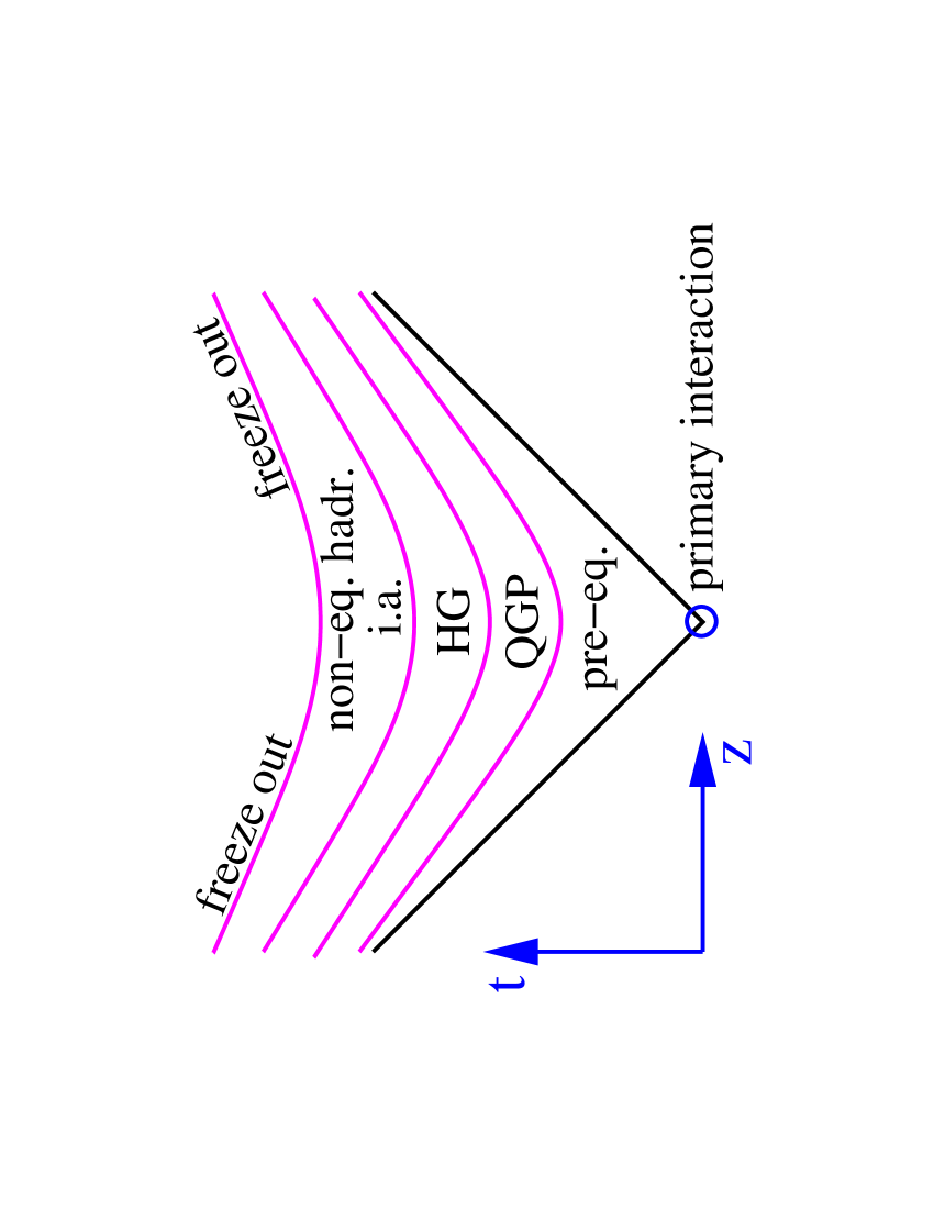
Figure 1: The different stages of heavy ion collisions.

(see fig. 1) and try to understand them as well as possible. There is, first of all, the primary interaction when the two nuclei pass through each other. Since at very high energies the longitudinal size is, due to the gamma factor, almost zero (of the order 0.1 fm at RHIC), all the nucleons of the projectile interact with all the nucleons of the target instantaneously. In such a primary interaction many partons are created, which interact (in the pre-equilibrium stage) before reaching an equilibrium, referred to as quark-gluon plasma. The system then expands, passing via phase transition (or sudden crossover) into the hadron gas stage. The density decreases further till the collision rate is no longer large enough to maintain chemical equilibrium, but there are still hadronic interactions till finally the particles “freeze out”, i.e. they continue their way without further interactions.

The equilibrium stage is often treated macroscopically, by solving hydrodynamical equations. Here, usually very simplified initial conditions are used, like flat distributions in space-time rapidity. This could be done much better by calculating the initial conditions for the hydrodynamical evolution on the basis of a realistic model for the primary interactions.

We recently presented a completely new approach [1, 2, 3] for hadronic interactions and the initial stage of nuclear collisions, referred to as neXus, where we provide a rigorous treatment of the multiple scattering aspect. Questions of energy conservation are clearly determined by the rules of field theory, both for cross section and particle production calculations, which is not the case in all of the corresponding models used so far to calculate the initial stage. In addition, we introduced (currently only to leading order) so-called enhanced diagrams, responsible for screening and diffraction. It was not the idea to create another model with some more features, but to provide a model which is theoretically consistent, and therefore much more realistic than all the approaches used before. We are therefore using neXus in order to determine macroscopic quantities after the first stage, when the two nuclei have traversed each other, such that these quantities may be used as initial conditions for a macroscopic treatment of the later stages of the collision.

Calculating for example energy densities from a model like neXus or any other model for primary interactions, is not trivial. We know the momenta of all the partons and we may calculate the energy density of the partonic system on a given hyper-surface (constant $\tau$), as shown in fig. 2.

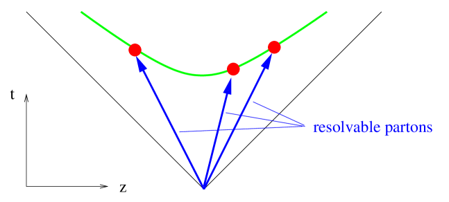
Figure 2: The naive method: only the resolvable partons are considered to determine the energy density on a hyper-surface (dots on hyperbola).

Here only the “resolvable” (or hard) partons are considered (dots on the hyperbola representing a hyper-surface). But this is certainly not the correct answer for the quantity of interest, since there are many “unresolved” (or soft) partons around, which contribute to the energy density in a significant fashion. The problem can be solved by using the string model, which is nothing but an attempt to treat the “soft partons” implicitly . The soft partons represent the string between “kinks”, the latter ones representing the hard partons, see fig. 3.

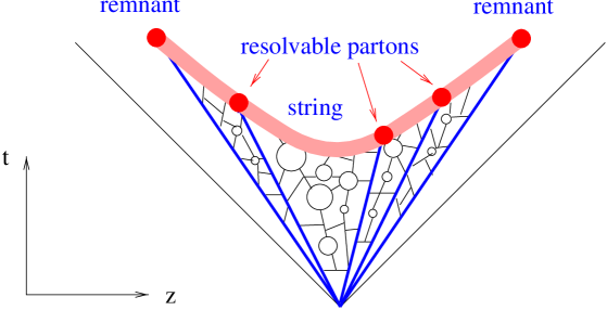
Figure 3: Between resolvable partons (thick lines) there are in addition unresolvable partons (thin lines), which are not treated explicitly. Their contribution is considered implicitly via strings.

Thus we are able to calculate energy densities in nucleus-nucleus collisions taking properly into account soft and hard (resolvable and unresolvable) contributions.

The outline of this paper is as follows: we first review briefly the basic elements of the neXus model, before we discuss in somewhat more detail the role of strings in this approach and the dynamics of strings. We then proceed to calculate energy densities for a given proper time, taking into account the hard and the soft partons.

2 The NEXUS Model

The most sophisticated approach to high energy hadronic interactions is the so-called Gribov-Regge theory [4]. This is an effective field theory, which allows multiple interactions to happen “in parallel”, with phenomenological objects called “Pomerons” representing elementary interactions [5]. Using the general rules of field theory, one may express cross sections in terms of a couple of parameters characterizing the Pomeron. Interference terms are crucial, as they assure the unitarity of the theory.

A big disadvantage is the fact that cross sections and particle production are not calculated consistently: the fact that energy needs to be shared between many Pomerons in case of multiple scattering is well taken into account when considering particle production (in particular in Monte Carlo applications), but not for cross sections [6].

Another problem is the fact that at high energies, one also needs a consistent approach to include both soft and hard processes. The latter ones are usually treated in the framework of the parton model, which only allows the calculation of inclusive cross sections.

We recently presented a completely new approach [1, 2, 3] for hadronic interactions and the initial stage of nuclear collisions, which is able to solve several of the above-mentioned problems. We provide a rigorous treatment of the multiple scattering aspect, such that questions of energy conservation are clearly determined by the rules of field theory, both for cross section and particle production calculations. In both (!) cases, energy is properly shared between the different interactions happening in parallel. This is the most important new aspect of our approach, which we consider a first necessary step to construct a consistent model for high energy nuclear scattering.

We first consider $pp$ scattering. An elementary interaction is given as a sum of soft, semi-hard, and hard contributions: $T_{2\rightarrow 2}=T_{\mathrm{soft}}+T_{\mathrm{semi}}+T_{\mathrm{hard}}$, as discussed in detail in ref. [3]. We have a hard contribution $T_{\mathrm{hard}}$, when the the first partons on both sides are valence quarks, a semi-hard contribution $T_{\mathrm{semi}}$, when at least on one side there is a sea quark (being emitted from a soft Pomeron), and finally we have a soft contribution, when there is no hard scattering at all (see fig. 4).

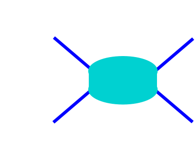
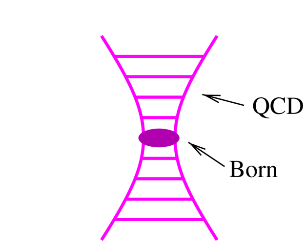
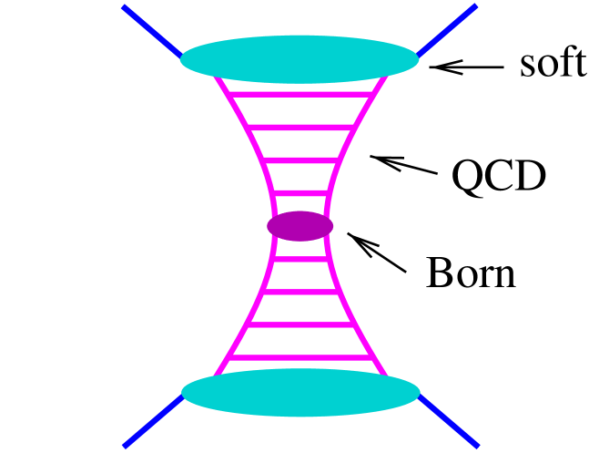
Figure 4: The soft elastic scattering amplitude $T_{\mathrm{soft}}$ (left), the hard elastic scattering amplitude $T_{\mathrm{hard}}$ (middle) and one of the three contributions to the semi-hard elastic scattering amplitude $T_{\mathrm{semi}}$ (right).

$T_{\mathrm{hard}}$ is calculated using the standard techniques of perturbative QCD, $T_{\mathrm{soft}}$ is parameterized, and $T_{\mathrm{semi}}$ is calculated as a convolution of $T_{\mathrm{soft}}$ and $T_{\mathrm{hard}}$. We have a smooth transition from soft to hard physics: at low energies the soft contribution dominates, at high energies the hard and semi-hard ones, at intermediate energies (that is where experiments are performed presently) all contributions are important.

Let us consider nucleus-nucleus ($AB$) scattering. The nucleus-nucleus scattering amplitude is defined by the sum of contributions of diagrams, corresponding to multiple elementary scattering processes between parton constituents of projectile and target nucleons. These elementary scatterings are the sum of soft, semi-hard, and hard contributions: $T_{2\rightarrow 2}=T_{\mathrm{soft}}+T_{\mathrm{semi}}+T_{\mathrm{hard}}$. A corresponding relation holds for the inelastic amplitude $T_{2\rightarrow X}$. We introduce “cut elementary diagrams” as being the sum over squared inelastic amplitudes, $\sum_{X}(T_{2\rightarrow X})$$(T_{2\rightarrow X})^{*}$, which are graphically represented by vertical dashed lines, whereas the elastic amplitudes are represented by unbroken lines:

   $=T_{2\rightarrow 2}$,           $=\sum_{X}(T_{2\rightarrow X})$$(T_{2\rightarrow X})^{*}$.

This is very handy for treating the nuclear scattering model. We define the model via the elastic scattering amplitude $T_{AB\rightarrow AB}$ which is assumed to consist of purely parallel elementary interactions between partonic constituents, described by $T_{2\rightarrow 2}$. The amplitude is therefore a sum of many terms. Having defined elastic scattering, inelastic scattering and particle production is practically given, if one employs a quantum mechanically self-consistent picture. Let us now consider inelastic scattering: one has of course the same parallel structure, just some of the elementary interactions may be inelastic, some elastic. The inelastic amplitude being a sum over many terms – $T_{AB\rightarrow X}=\sum_{i}T^{(i)}_{AB\rightarrow X}$ – has to be squared and summed over final states in order to get the inelastic cross section, which provides interference terms $\sum_{X}(T^{(i)}_{AB\rightarrow X})(T^{(j)}_{AB\rightarrow X})^{*}$. These can be conveniently expressed in terms of the cut and uncut elementary diagrams, as shown in fig. 5.

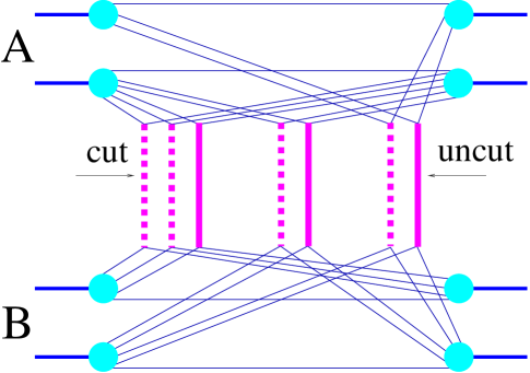
Figure 5: Example of a cut multiple scattering diagram, with cut (dashed lines) and uncut (full lines) elementary diagrams (Pomerons).

One has to be careful about energy conservation: all the partonic constituents (lines) leaving a nucleon (blob) have to share the momentum of the nucleon. So, in the explicit formula one has an integration over momentum fractions of the partons, taking care of momentum conservation. This formula is the master formula of the approach, allowing calculations of cross sections as well as particle production. In the latter case, the master formula provides probability distributions for the momenta taken by the Pomerons and the remnants. A very detailed description with many applications and comparisons with data can be found in [3].

So far we described only the basic version of the model. In reality we also consider triple Pomeron vertices to lowest order, as discussed in detail in ref. [3]. We do not yet consider higher orders, nor do we consider the case where the two legs of the triple Pomeron are connected to different nuclei. All this is work in progress.

3 Hadronic Structure of Cut Pomerons

In order to develop our multiple scattering theory, we use a simple graphical representation of a cut Pomeron, namely a thick vertical dashed line connecting the external legs representing nucleon components,

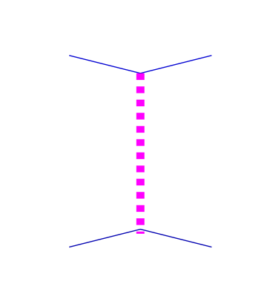
Figure 6: Symbol representing a cut Pomeron.

as shown in fig. 6. This simple diagram hides somewhat the fact that there is a complicated structure hidden in this Pomeron, and the purpose of this section is to discuss in particular the internal structure of the Pomeron.

Let us start our discussion with the soft Pomeron. Based on Veneziano’s topological expansion one may consider a soft Pomeron as a “cylinder”, i.e. the sum of all possible QCD diagrams having a cylindrical topology, see fig. 7.

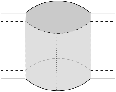
Figure 7: Cut soft Pomeron represented as a cut cylinder. The grey areas represent unresolved partons.

As discussed in detail in [3], the “nucleon components” mentioned earlier, representing the external legs of the diagram, are always quark-anti-quark pairs, indicated by a dashed line (anti-quark) and a full line (quark) in fig. 7. Important for the discussion of particle production are of course cut diagrams, therefore we show in fig. 7 a cut cylinder representing a cut Pomeron: the cut plane is shown as two vertical dotted lines. Let us consider the half-cylinder, for example, the one to the left of the cut, representing an inelastic amplitude.

Figure 8: Planar representation of a half-cylinder obtained from cutting a cylinder diagram (see fig. 7).

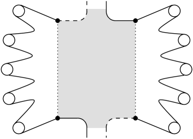
Figure 9: The string model: each cut line (dotted vertical lines) represents a string, which decays into final state hadrons (circles).

We may unfold this object in order to have a planar representation, as shown in fig. 8. Here, the dotted vertical lines indicate the cuts of the previous figure, and it is there where the hadronic final state hadrons appear. Lacking a theoretical understanding of this hadronic structure, we simply apply a phenomenological procedure, essentially a parameterization. We require the method to be as simple as possible, with a minimum of necessary parameters. A solution coming close to these demands is the so-called string model: each cut line is identified with a classical relativistic string. A Lorentz invariant string breaking procedure provides the transformation into a hadronic final state, see fig. 9.

The phenomenological microscopic picture which stays behind this procedure was discussed in a number of reviews [7, 8, 9]: the string end-point partons resulted from the interaction appear to be connected by a color field. With the partons flying apart, this color field is stretched into a tube, which finally breaks up giving rise to the production of hadrons and to the neutralization of the color field.

We now consider a semi-hard Pomeron of the “sea-sea” type, where we have a hard pQCD process in the middle and a soft evolution at the end, see fig. 10.

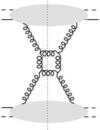
Figure 10: A simple diagram contributing to the semi-hard Pomeron of the “sea-sea” type.

We generalize the picture introduced above for the soft Pomeron. Again, we assume a cylindrical structure. For the example of fig. 10, we have the picture shown in fig. 11: the shaded areas on the cylinder ends represent the soft Pomerons, whereas in the middle part we draw explicitly the gluon lines on the cylinder surface. We apply the same procedure as for the soft Pomeron: we cut the diagram and present a half-cylinder in a planar fashion, see fig. 11.

            

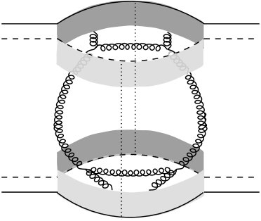
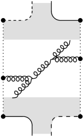
Figure 11: Cylindrical representation of a contribution to the semi-hard Pomeron (left figure) and planar diagram representing the corresponding half-cylinder (right figure).

We observe one difference compared to the soft case: there are three partons (dots) on each cut line: apart from the quark and the anti-quark at the end, we have a gluon in the middle. We again apply the string picture, but here we identify a cut line with a so-called kinky string, where the internal gluons correspond to internal kinks. The underlying microscopic picture will be presented by three color-connected partons - the gluon connected by the color field to the quark and to the anti-quark. The string model provides then a “parameterization” of hadron production, see fig. 12.

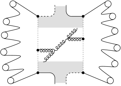
Figure 12: The “kinky” string model: the cut line (vertical dotted line) corresponds to a kinky string, which decays into hadrons (circles).

The procedure described above can be easily generalized to the case of complicated parton ladders involving many gluons and quark-anti-quark pairs. One should note that the treatment of semi-hard Pomerons is just a straightforward generalization of the string model for soft Pomerons, or one might see it the other way round: the soft string model is a natural limiting case of the kinky string procedure for semi-hard Pomerons. In a similar way one may treat Pomerons of valence type.

The general picture should be clear from the above examples: in any case, no matter what type of Pomeron, unresolved soft partons play a very important role. In the string model, they represent the string pieces between the hard partons. In case of single Pomeron exchange in proton-proton scattering, particle production can be treated in a phenomenological fashion via the hadronization of two (in general kinky) strings. In nuclear collisions, the situation is more complicated, since we have many Pomerons and consequently many strings – closely packed – which interact with each other. Nevertheless, we can use the string picture to calculate energy densities, by considering the strings at an earlier stage, before they hadronize.

It should be noted finally that particle production from cut Pomerons is not the whole story. Cutting the complete diagram, one has as well to cut the projectile and target remnants, which may or not be excited. High mass excitations are as well considered as strings.

4 Dynamics of Strings

The string dynamics is derived from the Nambu-Goto Lagrangian, which has been constructed based on invariance arguments. The corresponding equation of motion for the string is a wave equation, with a solution [10, 11, 12, 3]

$$X(r,t)=X_{0}+\frac{1}{2}\left[\int_{r-t}^{r+t}g\left(\xi\right)d\xi\right],$$ (1)

for the four-vector $X(r,t)$, having already assumed that the initial spatial extension of the string is zero. The quantity $X_{0}$ represents the formation point of the string, which coincides with the position of the nucleon-nucleon interaction being at the origin of the string formation. The space-like variable $r$ represents the position along the string for given time $t$, whereas the function $g$ defines the initial velocity,

$$g(r)=\dot{X}(r,t)|_{t=0}.$$ (2)

We will consider here a special class of strings, namely those with a piecewise constant function $g$,

$$g(r)=v_{k}\quad\;\mathrm{for}\>\frac{E_{k-1}}{\kappa}\leq r\leq\frac{E_{k}}{\kappa},\quad\;1\leq k\leq n$$ (3)

for some integer $n$. We use for the string tension $\kappa=1$ GeV/fm. The set $\{E_{k}\}$ is a partition of the interval $[0,E]$, with $E$ being the string energy,

$$0=E_{0}<E_{1}<...<E_{n-1}<E_{n}=E,$$ (4)

and $\{v_{k}\}$ represents $n$ constant 4-vectors. Such strings are called kinky strings, with $n$ being the number of kinks, and the $n$ vectors $v_{k}$ being called kink velocities. The function $g$ must be symmetric and periodic, with the period $2E/\kappa$. This defines $g$ everywhere, and eq. (1) is the complete solution of the string equation, expressed in terms of the initial condition $g$. In the case of kinky strings the latter is expressed in terms of the kink velocities $\{v_{k}\}$ and the energy partition $\{E_{k}\}$.

What has all this to do with cut Pomerons? So far nothing, and to establish a link, we have to provide some mapping from the language of Pomerons and partons into the language of strings. We discussed earlier that a cut Pomeron may be identified with two sequences of partons of the type

$$q-g-g-...-g-\bar{q},$$ (5)

representing all the partons on a cut line. We identify such a sequence with a kinky string, by requiring

$$\mathrm{parton}=\mathrm{kink},$$ (6)

which means we identify the partons of the above sequence with the kinks of a kinky string, such that the partition of the energy is given by the parton energies,

$$E_{k}=\mathrm{energy}\,\mathrm{of}\,\mathrm{parton}\,k$$ (7)

and the kink velocities are just the parton velocities,

$$v_{k}=\frac{\mathrm{momentum}\,\mathrm{of}\,\mathrm{parton}\,k}{E_{k}}.$$ (8)

We consider massless partons, so that the energy is equal to the absolute value of the parton momentum.

Figure 13: Partons of an $e^{+}e^{-}$ annihilation event with $\sqrt{s}=14\textrm{ GeV}$ in the $z-x$ plane. The figure in the left upper corner shows the momenta in the $p_{z}-p_{x}$ plane.

An example is shown on fig. 13, we have 6 partons – a quark and an anti-quark, with 4 gluons in between – symbolically displayed in the first sub-figure, with a total cms energy of 14 GeV. One sees that the perturbative gluons play an important role in the beginning of the movement, and later from 2 GeV on, the longitudinal character dominates. A string breaks typically after $1\textrm{ GeV}/\kappa$, with $\kappa$ being the string tension, which gives much importance to the perturbative gluons.

5 Energy Densities from Strings

Based on the string formalism, we are now able to calculate energy densities. As discussed above, a string $S$ is a two-dimensional surface $X(r,t)$ in Minkowski space, whose intersection with the surface

$$t^{2}-z^{2}=\tau^{2}$$ (9)

defines uniquely a curve $S_{\tau}$, which we refer to as “String at given proper time $\tau$”. Our aim is to calculate the energy density and the velocity flow at a given proper time $\tau$, in other words, along the curve $S_{\tau}$.

Let us consider a small string piece $\Delta S_{\tau}$, in other words a segment of the string curve $S_{\tau}$ between two neighboring points $A$ and $B$, being sufficiently close so that the string piece may be considered as point-like. According to relativistic string theory, the four-momentum of this string piece in the lab system is given as

$$\Delta P_{\mathrm{lab}}=\int_{A}^{B}\left\{\frac{\partial X(r,t)}{\partial t}dr+\frac{\partial X(r,t)}{\partial r}dt\right\}.$$ (10)

The partial derivatives can be expressed in terms of the initial velocity $g$ as

$$\frac{\partial X(r,t)}{\partial t} = \frac{1}{2}\left[g(r+t)+g(r-t)\right]$$ (11)

$$\frac{\partial X(r,t)}{\partial r} = \frac{1}{2}\left[g(r+t)-g(r-t)\right]\,\,.$$ (12)

This velocity function is known, in fact it is defined via the mapping of a system of $n$ partons into string language:

$$g(r)=v_{k}\quad\;\mathrm{for}\>\frac{E_{k-1}}{\kappa}\leq r\leq\frac{E_{k}}{\kappa},\quad\;1\leq k\leq n,$$ (13)

where $v_{k}$ is the four-velocity of the $k^{\mathrm{th}}$ parton divided by $\gamma$, and the difference $E_{k}-E_{k-1}$ is its energy. So the four-momentum of a string segment can be easily expressed in terms of the original parton momenta.

We use hyperbolic coordinates,

$$q_{0}=\tau=\sqrt{t^{2}-z^{2}},\qquad q_{1}=x,\qquad q_{2}=y,\qquad q_{3}=\eta=\frac{1}{2}\log\frac{1+z/t}{1-z/t},$$ (14)

where $z$ is considered to be the coordinate along the beam axis, and $t$ is the time. The variables $x$ and $y$ are the transverse coordinates. For given $\tau$ and $\eta$, we define a frame $F_{\eta}$ via a Lorentz boost with boost rapidity $\eta$. The four-momentum of the above-mentioned string piece is given as

$$\Delta P^{\mu}=\Lambda_{\nu}^{\mu}\,\Delta P_{\mathrm{lab}}^{\nu}\,,$$ (15)

with the corresponding transformation tensor $\Lambda$.

We are now going to calculate the energy momentum tensor $T^{\mu\nu}$ for a string piece in the frame $F_{\eta}$. The general definition in kinetic theory is

$$T^{\mu\nu}(\vec{q})=\int\frac{d^{3}p}{E}p^{\mu}p^{\nu}f(\vec{q},\vec{p}),$$ (16)

where $\vec{q}$ is a position four-vector, and $f$ the phase space density (particles per phase space volume) for a given time. For our point-like string piece we have in principle

$$f(\vec{q},\vec{p})=\delta(\vec{p}-\overrightarrow{\Delta P})\delta(\vec{q}-\vec{Q}).$$ (17)

Knowing that a string with zero width is a mathematical idealization, we introduce a Gaussian-type smearing function $W(q)$, normalized as $\int W(q)4\pi q^{2}dq=1$. So we define

$$f(\vec{q},\vec{p})=\delta(\vec{p}-\overrightarrow{\Delta P})W\left(\left\|\vec{q}-\vec{Q}\right\|\right),$$ (18)

with the norm in hyperbolic coordinates being given as

$$\left\|\vec{q}\right\|=\left(q_{1}\right)^{2}+\left(q_{2}\right)^{2}+\tau^{2}\left(q_{3}\right)^{2}.$$ (19)

The energy momentum tensor for the complete string is then just the sum over all string pieces, which gives

$$T^{\mu\nu}(\vec{q})=\sum_{\mathrm{string}\,\mathrm{segments}}\frac{\Delta P^{\mu}\Delta P^{\nu}}{P^{0}}\,W\left(\left\|\vec{q}-\vec{Q}\right\|\right).$$ (20)

We define a local comoving frame via the four-velocity

$$u^{\mu}(\vec{q})=\frac{n^{\mu}(\vec{q})}{\sqrt{n^{\mu}(\vec{q})\,n_{\mu}(\vec{q})}}$$ (21)

with

$$n^{\mu}(\vec{q})=T^{0\mu}(\vec{q}).$$ (22)

This allows then the calculation of the energy density in the comoving frame,

$$\epsilon(q)=T^{\mu\nu}(\vec{q})\,u_{\mu}(\vec{q})\,u_{\nu}(\vec{q}),$$ (23)

and the flow velocity

$$\vec{v}(q)=\vec{u}(q)/u^{0}.$$ (24)

6 Results

In the following, we show results for different high energy reactions. All the calculations are done at the proper time $\tau=$ 1fm/c, and we suppress writing this variable in the following. We use always a width $\sigma=0.5\textrm{fm}$ for smearing function $W(q)$. We define the rapidity field $y_{z}(x,y,\eta)$ as

$$y_{z}(x,y,\eta)=\frac{1}{2}\log\frac{1+v_{z}(x,y,\eta)}{1-v_{z}(x,y,\eta)},$$ (25)

where $v_{z}(x,y,v_{z})$ is the $z$ component of the velocity field.

As a reference, we first show results for a single string without kinks, having an energy of 50 GeV, as it may occur in electron-positron annihilation. In fig. 14, we plot the energy density $\epsilon(x,y,\eta)$ as a function of $x$ and $\eta$ for $y=0$. As expected, the energy density is peaked around $x=0$, whereas it is distributed evenly in $\eta$ between limits defined by the energy of the string. Since there is a cylindrical symmetry with respect to the $z$ axis, it is no surprise that the energy density as a function of $x$ and $y$ for $\eta=0$ shows a narrow peak around $x=y=0$, as seen in fig. 15. The rapidity field $y_{z}(x,y,\eta)$ as a function of $x$ and $\eta$ for $y=0$ is shown in fig. 16, where we observe roughly $y_{z}(x,y,\eta)=\eta$. The other components of the velocity field are zero.

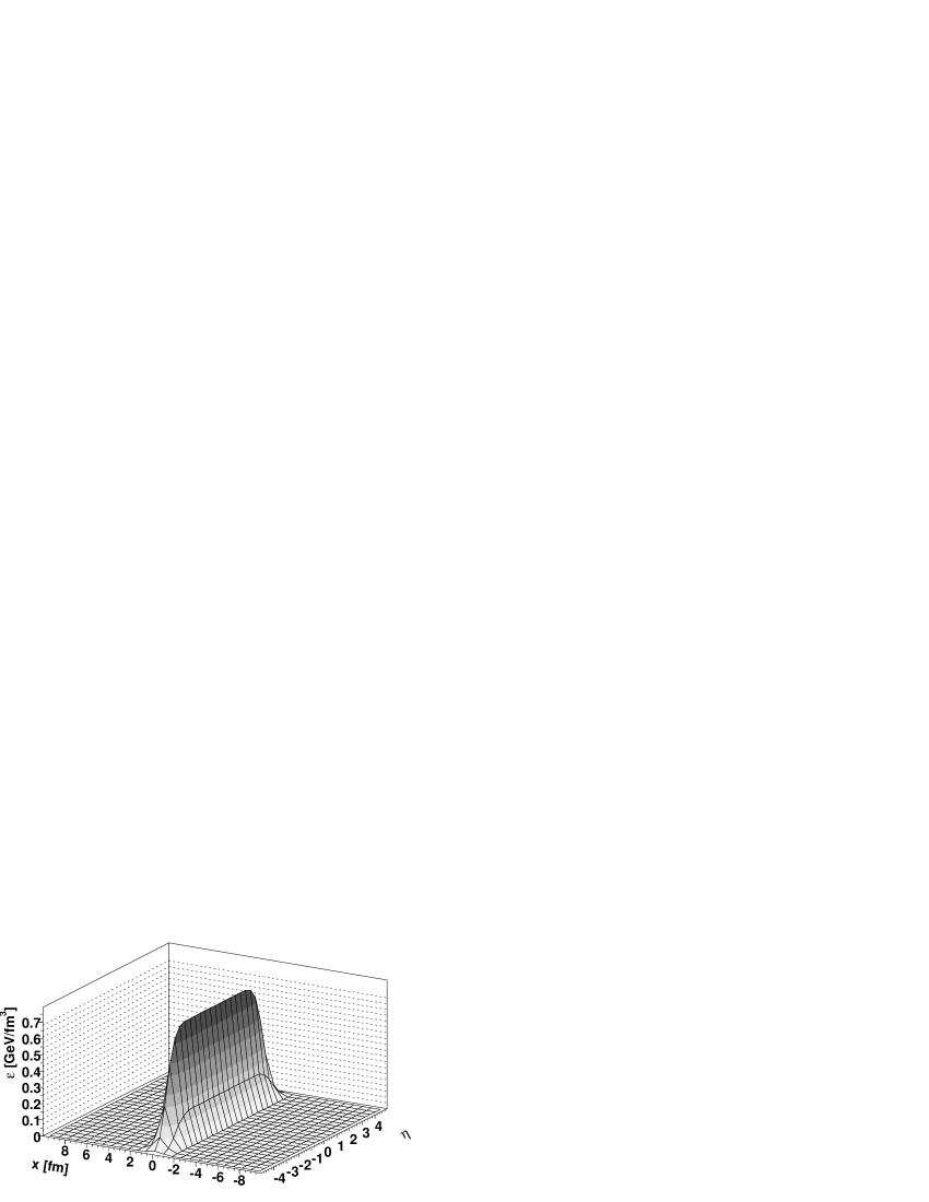
Figure 14: Energy density in the $x-\eta$ plane at $y=0$ for a single string of energy 50 GeV.

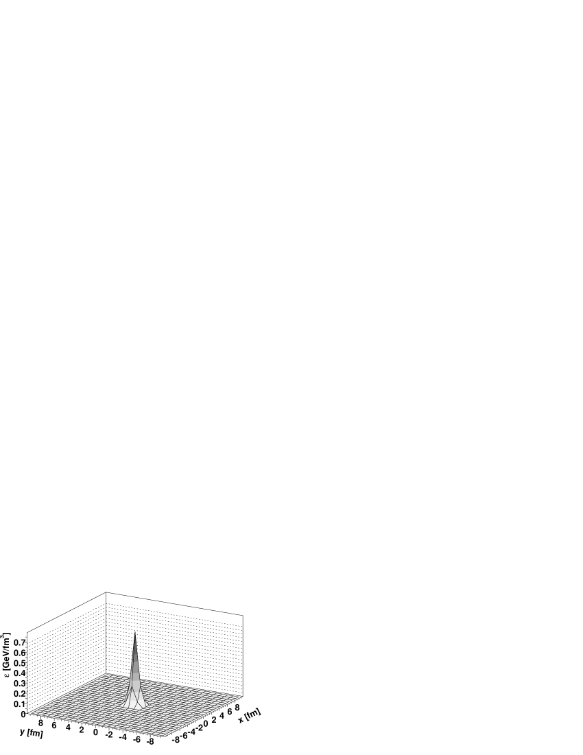
Figure 15: Energy density in the $x-y$ plane at $\eta=0$ for a single string of energy 50 GeV.

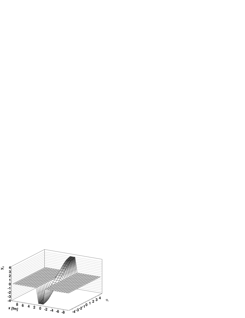
Figure 16: Rapidity field in the $x-\eta$ plane at $y=0$ for a single string of energy 50 GeV.

Kinky strings show a very similar behavior. Due to the transverse momenta introduced via the kinks, the cylindrical symmetry is slightly distorted, and we observe as well very small but finite values for the transverse components of the velocity fields.Since the results are so close to the simple string discussed above, we do not show the figures here.

Next we consider proton-proton scattering at 50 GeV.

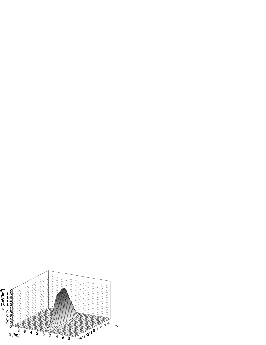
Figure 17: Energy density in the $x-\eta$ plane at $y=0$ for a proton-proton collision at 50 GeV.

Figure 18: Energy density in the $x-y$ plane at $\eta=0$ for a proton-proton collision at 50 GeV.

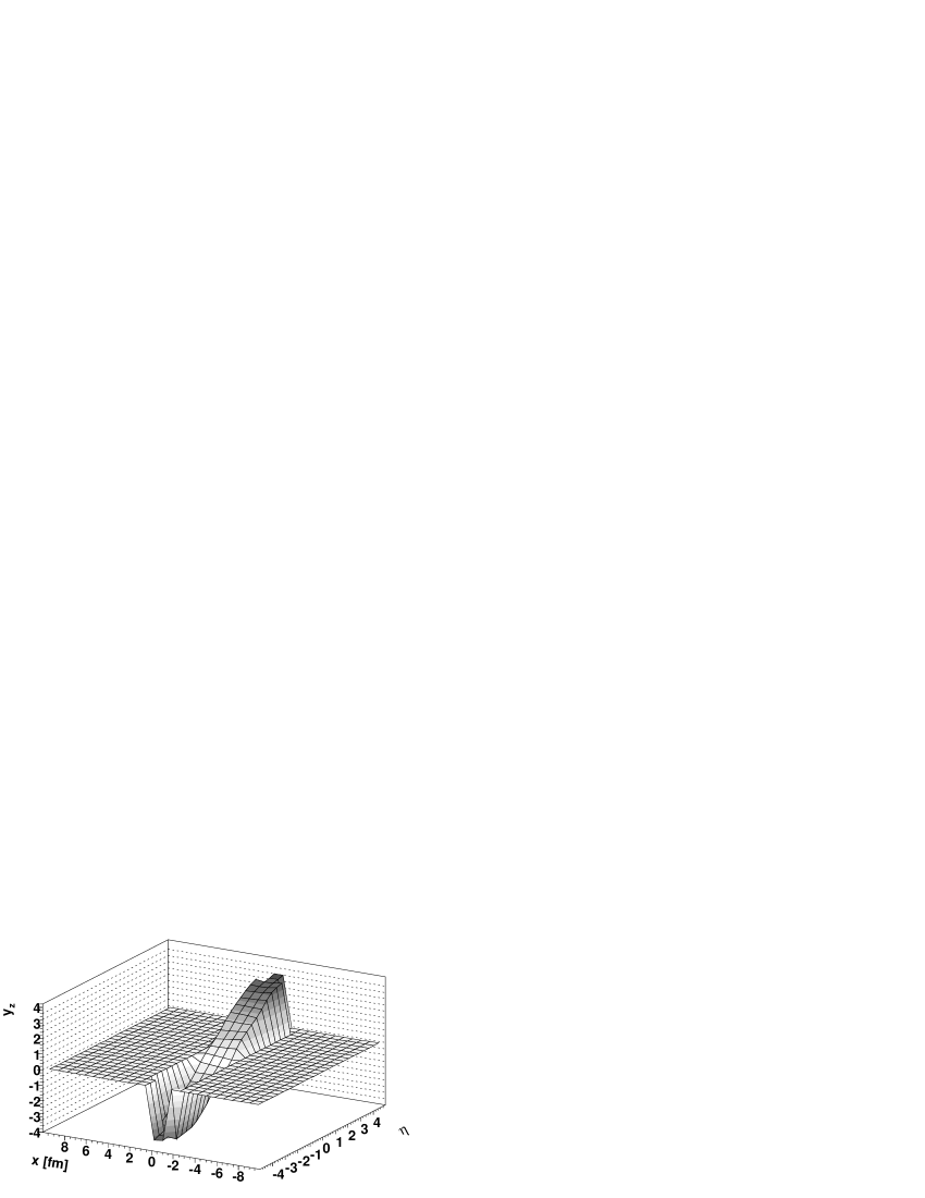
Figure 19: Rapidity field in the $x-\eta$ plane at $y=0$ for a proton-proton collision at 50 GeV.

Here we have usually several strings, the minimum number being two, plus two remnants (which may be strings in case of high mass excitation). In the example considered here, we have altogether four strings, with respective energies of 17.2 GeV, 9.3 GeV, 7.6 GeV and 15.8 GeV. Since the strings have different masses and are not sitting in the cms system, the energy density $\epsilon(x,y,\eta)$ as a function of $x$ and $\eta$ for $y=0$ does not show such a flat behavior as in the case of a pure string, as seen in fig. 17, but we observe a peak at $\eta=0$, whose value is roughly 2.5 times bigger than the one for a string. However, the energy density as a function of $x$ and $y$ for $\eta=0$ shows as well a narrow peak around $x=y=0$, as shown in fig. 18, and the rapidity field $y_{z}(x,y,\eta)$ is roughly equal to $\eta$ , see fig. 19.

Let us consider gold-gold collisions at RHIC (200 AGeV). In fig. 20,

Figure 20: Energy density in the $x-\eta$ plane at $y=0$ for a central gold-gold collision at 200 AGeV.

we show the energy density $\epsilon(x,y,\eta)$ as a function of $x$ and $\eta$ for $y=0$. For a fixed value of $x$, we observe a similar shape as for proton-proton scattering: a broad distribution with a smooth peak around zero. Of course, the magnitude is much bigger. Considering, however, the variation with $x$ for given $\eta$, we observed large fluctuations: pronounced peaks followed by deep valleys. If we regard the energy density as a function of $x$ and $y$ for $\eta=0$, as shown in fig. 21,

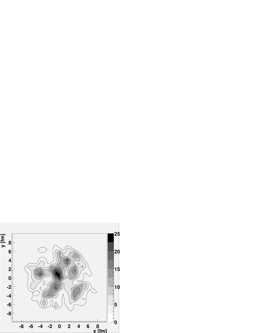
Figure 21: Energy density in the $x-y$ plane at $\eta=0$ for a central gold-gold collision at 200 AGeV.

we observe correspondingly several peaks overlaying the general roughly rotationally symmetric structure, which increases towards the center. To investigate the origin of these fluctuations, we show in fig. 22 the distribution of the number of

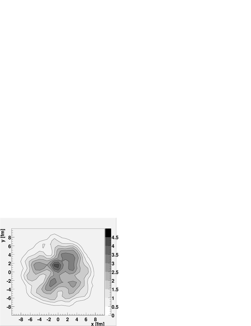
Figure 22: Projected nucleon density in the $x-y$ plane for a central gold-gold collision at 200 AGeV.

nucleons (projectile plus target) projected to the plane $z=0$, in units nucleons per $\mathrm{fm}^{2}$. From a spherically symmetric nuclear density, we expect a rotationally symmetric distribution of this projection, increasing towards the center ($x=y=0$). This is also what one observes, roughly. But looking more closely, we clearly observe large fluctuations with pronounced peaks. And even more, these peaks correspond exactly to the peaks in the energy density distribution, which proves that the fluctuations in energy density are due to geometrical fluctuations in the distribution of nucleons.

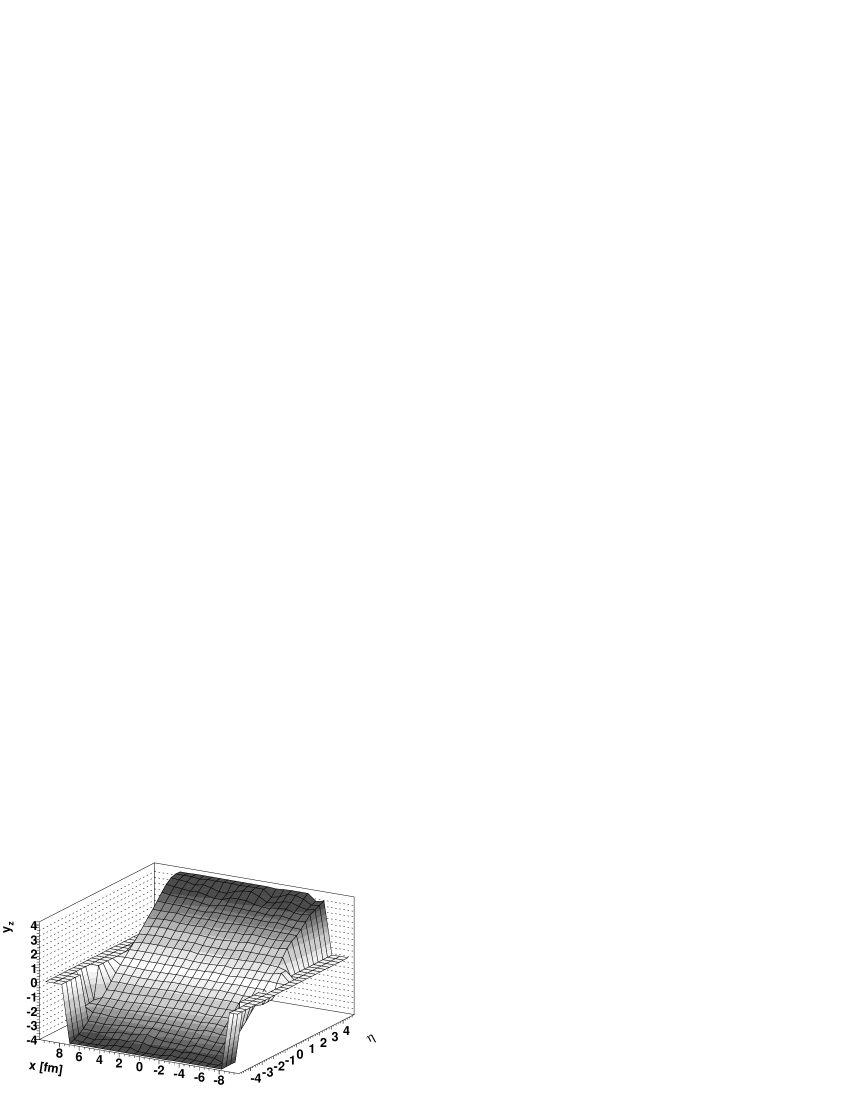
Figure 23: Rapidity field in the $x-\eta$ plane at $y=0$ for a central gold-gold collision at 200 AGeV.

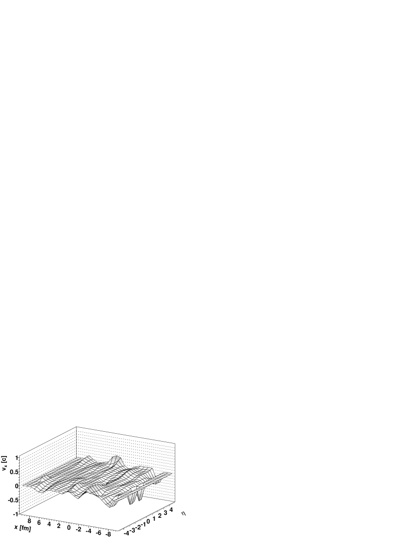
Figure 24: Velocity field ($x$-component) in the $x-\eta$ plane at $y=0$ for a central gold-gold collision at 200 AGeV.

We finally consider rapidity and velocity fields: in fig. 23 the rapidity field $y_{z}(x,y,\eta)$ and in fig. 24 the $x$ component $v_{x}(x,y,\eta)$ of the velocity field, both as a function of $x$ and $\eta$ for $y=0$. We observe roughly $y_{z}=\eta$ and $v_{x}$ close to zero. So the velocity field is practically purely longitudinal and shows the so-called “Bjorken scaling” ($y_{z}=\eta$).

7 Summary

We presented a new way to calculate macroscopic quantities like energy density or velocity (or rapidity) fields at an early stage of a nucleus-nucleus collision at ultra-relativistic energies. The calculation is based on a sophisticated treatment of the primary interactions, when the two nuclei are traversing each other, using the parton-based Gribov-Regge model neXus. The important point is an appropriate treatment of soft partons, which contribute substantially and which are usually completely neglected. In neXus, soft and hard physics are considered consistently: hard partons are treated explicitly based on pQCD, soft ones are included implicitly, using the string picture. This allows a quite reliable calculation of the above-mentioned macroscopic quantities.

We analyzed single strings, proton-proton scattering and heavy ion collisions. In the latter case, we find almost perfect “Bjorken scaling”: the rapidity $y_{z}$ coincides with the space-time rapidity $\eta$, whereas the transverse flow is practically zero. This is often employed as initial condition for hydrodynamical treatments. However, the $\eta$ dependence of the energy density does not show a well defined plateau corresponding to “boost invariance”. Furthermore, the distribution of the energy density in the transverse plane shows typically a very “bumpy” structure, which fluctuates considerably from event to event.

This work has been funded in part by the IN2P3/CNRS (PICS 580) and the Russian Foundation of Basic Researches (RFBR-98-02-22024). H.J.D. acknowledges support from NASA grant number NAG-9246.

References

- [1] K. Werner, H. Drescher, E. Furler, M. Hladik, and S. Ostapchenko, Semihard processes in nuclear collisions, in Proc. of the "3rd International Conference on Physics and Astrophysics of Quark-Gluon Plasma", Jaipur, India, March 17-21, 1997, 1997.
- [2] H. J. Drescher, M. Hladik, S. Ostapchenko, and K. Werner, Nucl. Phys. A661, 604 (1999), hep-ph/9906428.
- [3] H. J. Drescher, M. Hladik, S. Ostapchenko, T. Pierog, and K. Werner, (2000), hep-ph/0007198, to be published in Physics Reports.
- [4] V. N. Gribov, Sov. Phys. JETP 26, 414 (1968).
- [5] M. Baker and K. A. Ter-Martirosyan, Phys. Rep. 28, 1 (1976).
- [6] V. A. Abramovskii and G. G. Leptoukh, Sov.J.Nucl.Phys. 55, 903 (1992).
- [7] A. B. Kaidalov and K. A. Ter-Martirosyan, Phys. Lett. 117B, 247 (1982).
- [8] A. Capella, U. Sukhatme, C.-I. Tan, and J. Tran Thanh Van, Phys. Rept. 236, 225 (1994).
- [9] B. Andersson, G. Gustafson, G. Ingelman, and T. Sjostrand, Phys. Rept. 97, 31 (1983).
- [10] Y. Nambu, Proc. Intl. Conf. on Symmetries and Quark Models Wayne State Univ., 1969.
- [11] C. Rebbi, Phys. Rept. 12, 1 (1974).
- [12] J. Scherk, Rev. Mod. Phys. 47, 123 (1975).