RUB-TP2-20/00

Abstract

We show that in the large $N_{c}$ limit four-quark twist-4 distributions in the pion can be expressed in terms of twist-2 pion distribution amplitude. This allows us to compute the isospin-2 structure function of the pion $F_{2}^{I=2}(x_{B})$ in the large $N_{c}$ limit. The method can be easily applied to other mesons as well.

1. Matrix elements of four-quark operators appear e.g. in twist-4 contributions to the structure functions of deep–inelastic scattering [1, 2], or in the description of non-leptonic weak decays [3]. In this paper we consider the specific example of isospin-2 pion structure functions $F_{2}(x_{B})$

$$F_{2}^{I=2}=F_{2}^{\pi^{+}}+F_{2}^{\pi^{-}}-2F_{2}^{\pi^{0}}\,.$$ (1)

In this particular isospin combination of structure functions the contribution of twist-2 operators cancels out exactly and twist-4 contributions are dominant. It is remarkable that in the large $N_{c}$ limit the twist-4 distribution function of quarks in the pion can be reduced to a convolution of twist-2 pion distribution amplitudes.

2. One can read the contribution of four-quark twist-4 operators to $F_{2}$ from [4, 5] (correcting obvious misprints)

$$\frac{1}{x_{B}}F_{2}^{twist-4}(x_{B})=\frac{1}{Q^{2}}\int dx_{1}dxdx_{2}\,x_{B}$$

$$\times\left\{\left[\Delta(x_{2},x_{1},x)+\Delta(y_{2},y_{1},x)\right]T_{qq}^{(+)}(x_{1},x,x_{2})\right.$$

$$\left.-\left[\Delta(x_{2},y_{1},x)+\Delta(y_{2},x_{1},x)\right]T_{qq}^{(-)}(x_{1},x,x_{2})\right\}\,.$$ (2)

Here $y_{1}\equiv x-x_{1},\ y_{2}\equiv x-x_{2}$. We use the function $\Delta$ from ref. [4]

$$\Delta(x_{1},x_{2},x_{3})=-\frac{1}{\pi}{\rm Im}\Biggl{[}\frac{1}{x_{1}-x_{B}+i0}\,\frac{1}{x_{2}-x_{B}+i0}\,\frac{1}{x_{3}-x_{B}+i0}\Biggr{]}\,.$$ (3)

The functions $T_{qq}^{(\pm)}(x_{1},x,x_{2})$ are defined as follows

$$T_{qq}^{(\pm)}(x_{1},x,x_{2})=T_{qq}(x_{1},x,x_{2})\pm\tilde{T}_{qq}(x_{1},x,x_{2})$$ (4)

with $T_{qq}$, $\tilde{T}_{qq}$ given by

$$\left.\begin{array}[]{c}T_{qq}(x_{1},x,x_{2})\\ \tilde{T}_{qq}(x_{1},x,x_{2})\end{array}\right\}=g^{2}\frac{p^{+}}{4}\int\frac{dz_{1}^{-}}{2\pi}\,\frac{dz_{2}^{-}}{2\pi}\,\frac{dz^{-}}{2\pi}$$

$$\times\exp\left\{ip^{+}\left[x_{1}z_{1}^{-}+(x-x_{1})z^{-}-(x-x_{2})z_{2}^{-}\right]\right\}$$

$$\times\langle p|T\left\{\left[\bar{\psi}(0)\Gamma t^{B}\psi(z_{2}^{-})\right]\left[\bar{\psi}(z^{-})\Gamma t^{B}\psi(z_{1}^{-})\right]\right\}|p\rangle\,.$$ (5)

Here $g$ is the QCD coupling constant, $t^{B}=\frac{1}{2}\lambda^{B}$ are generators of the color group and

$$\Gamma=\left\{\begin{array}[]{cc}\gamma^{+}Q_{e}&{\rm for\ }T_{qq}\\ \gamma_{5}\gamma^{+}Q_{e}&{\rm for\ }\tilde{T}_{qq}\end{array}\right.\,,$$ (6)

where $Q_{e}$ is the quark electric charge matrix. The light-cone components of a vector $V^{\mu}$ are defined as $V^{\pm}=\frac{1}{\sqrt{2}}(V^{0}\pm V^{3})$.

3. Generically the meson matrix elements of four-quark twist-4 operators are not related to matrix elements of two-quark operators. Here we show that in the limit of large number of colors $N_{c}$ the matrix elements of four-quark operators can be expressed in terms of marix elements of two-quark operators. This observation allows us to express twist-4 contribution to $F_{2}(x)$ of the pion in terms of twist-2 distribution amplitudes.

A simple analysis of leading in $N_{c}$ Feynman diagrams [6], corresponding to the meson matrix element

$$\langle M_{1}|(\bar{\psi}O_{1}\psi)(\bar{\psi}O_{2}\psi)|M_{2}\rangle$$ (7)

with matrices $O_{i}$ being unity in the color subspace, shows that this matrix elements can be factorized in the limit of large number of colors as

$$\langle M_{1}|(\bar{\psi}O_{1}\psi)(\bar{\psi}O_{2}\psi)|M_{2}\rangle\stackrel{{\scriptstyle N_{c}\rightarrow\infty}}{{\longrightarrow}}\langle M_{1}|M_{2}\rangle\langle 0|(\bar{\psi}O_{1}\psi)(\bar{\psi}O_{2}\psi)|0\rangle$$

$$+\langle M_{1}|(\bar{\psi}O_{1}\psi)|0\rangle\,\langle 0|(\bar{\psi}O_{2}\psi)|M_{2}\rangle+\langle M_{1}|(\bar{\psi}O_{2}\psi)|0\rangle\,\langle 0|(\bar{\psi}O_{1}\psi)|M_{2}\rangle\,.$$ (8)

Let us define the connected part of the matrix element as follows

$$\langle M_{1}|(\bar{\psi}O_{1}\psi)(\bar{\psi}O_{2}\psi)|M_{2}\rangle_{connected}$$

$$\equiv\langle M_{1}|(\bar{\psi}O_{1}\psi)(\bar{\psi}O_{2}\psi)|M_{2}\rangle-\langle M_{1}|M_{2}\rangle\langle 0|(\bar{\psi}O_{1}\psi)(\bar{\psi}O_{2}\psi)|0\rangle\,.$$ (9)

If mesons $M_{1}$ and $M_{2}$ have different momenta or different internal quantum numbers then $\langle M_{1}|M_{2}\rangle=0$ and there is no difference between the matrix elements and its connected part. But if $|M_{1}\rangle=|M_{2}\rangle$ then the nonconnected matrix element $\langle M_{1}|(\bar{\psi}O_{1}\psi)(\bar{\psi}O_{2}\psi)|M_{2}\rangle$ is divergent and we must consider the connected part. Now the factorization (8) takes the form

$$\langle M_{1}|(\bar{\psi}O_{1}\psi)(\bar{\psi}O_{2}\psi)|M_{2}\rangle_{connected}$$

$$\stackrel{{\scriptstyle N_{c}\rightarrow\infty}}{{\longrightarrow}}\langle M_{1}|(\bar{\psi}O_{1}\psi)|0\rangle\,\langle 0|(\bar{\psi}O_{2}\psi)|M_{2}\rangle+\langle M_{1}|(\bar{\psi}O_{2}\psi)|0\rangle\,\langle 0|(\bar{\psi}O_{1}\psi)|M_{2}\rangle\,.$$ (10)

We want to investigate the large $N_{c}$ behavior of the pion distribution functions. They are defined in terms of matrix elements

$$\langle M_{1}|T\left\{\left[\bar{\psi}(z_{1}^{\prime})\Gamma_{1}t^{B}\psi(z_{1})\right]\left[\bar{\psi}(z_{2}^{\prime})\Gamma_{2}t^{B}\psi(z_{2})\right]\right\}|M_{2}\rangle\,.$$ (11)

We remind that

$${\rm Sp}(t^{A}t^{B})=\frac{1}{2}\delta^{AB}\,,$$ (12)

$$\sum\limits_{B}t_{ij}^{B}t_{kl}^{B}=\frac{1}{2}\left(\delta_{il}\delta_{jk}-\frac{1}{N_{c}}\delta_{ij}\delta_{kl}\right)\,.$$ (13)

In the large $N_{c}$ limit this reduces to

$$\sum\limits_{B}t_{ij}^{B}t_{kl}^{B}\rightarrow\frac{1}{2}\delta_{il}\delta_{jk}\,.$$ (14)

Hence for any color singlet matrices $\Gamma_{1,2}$ we have

$$\langle M_{1}|T\left\{\left[\bar{\psi}(z_{1}^{\prime})\Gamma_{1}t^{B}\psi(z_{1})\right]\left[\bar{\psi}(z_{2}^{\prime})\Gamma_{2}t^{B}\psi(z_{2})\right]\right\}|M_{2}\rangle$$

$$\stackrel{{\scriptstyle N_{c}\rightarrow\infty}}{{\longrightarrow}}-\frac{1}{2}\langle M_{1}|T\left\{{\rm Sp}\left[\psi(z_{2})\otimes\bar{\psi}(z_{1}^{\prime})\right]\Gamma_{1}\left[\psi(z_{1})\otimes\bar{\psi}(z_{2}^{\prime})\right]\Gamma_{2}\right\}|M_{2}\rangle\,.$$ (15)

We stress that here in $\bar{\psi}(z_{1}^{\prime})\otimes\psi(z_{2})$ the tensor product refers to the spin flavor indices while the color indices are contracted. The trace Sp also refers only to spin-flavor indices.

Applying the large $N_{c}$ factorization formula (10) to the matrix element in the rhs of (15) one obtains

$$\langle M_{1}|T\left\{\left[\bar{\psi}(z_{1}^{\prime})\Gamma_{1}t^{B}\psi(z_{1})\right]\left[\bar{\psi}(z_{2}^{\prime})\Gamma_{2}t^{B}\psi(z_{2})\right]\right\}|M_{2}\rangle_{connected}$$

$$\stackrel{{\scriptstyle N_{c}\rightarrow\infty}}{{\longrightarrow}}-\frac{1}{2}{\rm Sp}\left\{\langle M_{1}|T\left[\psi(z_{2})\otimes\bar{\psi}(z_{1}^{\prime})\right]|0\rangle\,\Gamma_{1}\,\langle 0|T\left[\psi(z_{1})\otimes\bar{\psi}(z_{2}^{\prime})\right]|M_{2}\rangle\,\Gamma_{2}\right\}$$

$$-\frac{1}{2}{\rm Sp}\left\{\langle 0|T\left[\psi(z_{2})\otimes\bar{\psi}(z_{1}^{\prime})\right]|M_{2}\rangle\,\Gamma_{1}\,\langle M_{1}|T\left[\psi(z_{1})\otimes\bar{\psi}(z_{2}^{\prime})\right]|0\rangle\,\Gamma_{2}\right\}\,.$$ (16)

Now we apply the general large $N_{c}$ eq. (16) to matrix elements entering in definitions of twist-4 parton distributions (5). We obtain the following result for these functions

$$T_{qq}^{(+)}(x_{1},x,x_{2})\equiv\left[T_{qq}(x_{1},x,x_{2})+\tilde{T}_{qq}(x_{1},x,x_{2})\right]$$

$$=-g^{2}\frac{F_{\pi}^{2}}{8}\left[\delta(x_{1}-x_{2}-1)\phi_{\pi}(x_{1}-x)\phi_{\pi}(x_{1})+\delta(x_{2}-x_{1}-1)\phi_{\pi}(x_{2}-x)\phi_{\pi}(x_{2})\right]$$

$$\times\left(-\frac{4}{9}\delta^{ab}+\delta^{a3}\delta^{b3}\right)\,.$$ (17)

Here $\phi_{\pi}(x)$ is the pion twist-2 distribution amplitude defined as

$$\frac{1}{F_{\pi}}\int\frac{d\lambda}{2\pi}e^{ix\lambda(P\cdot n)}\langle 0|\bar{\psi}(\lambda n)\hat{n}\gamma_{5}\frac{\tau^{b}}{2}\psi(0)|\pi^{a}(P)\rangle=i\delta^{ab}\phi_{\pi}(x)\,.$$ (18)

Here $F_{\pi}\approx 93$ MeV is the pion decay constant and $a,b$ are isospin indices. Also it is easy to see from definition eqs. (4,5) that at leading order of the $1/N_{c}$ expansion

$$T_{qq}^{(-)}(x_{1},x,x_{2})=0\,.$$ (19)

We see that in the large $N_{c}$ limit the meson twist-4 four-quark distributions are expressible in terms of twist-2 meson distribution amplitudes. Now we are in a position to compute the twist-4 part of $F_{2}(x_{B})$. We insert expressions (17,19) into eq. (2)

$$F_{2}^{twist-4}(x_{B})=-g^{2}\frac{x_{B}^{2}}{Q^{2}}\,\frac{F_{\pi}^{2}}{4}\left(-\frac{4}{9}\delta^{ab}+\delta^{a3}\delta^{b3}\right)$$

$$\times\left\{2\phi_{\pi}(x_{B})\int dx_{1}\phi_{\pi}(x_{1})\frac{1}{x_{1}}\right.$$

$$\left.-\int dx_{1}dy_{1}\phi_{\pi}(y_{1})\phi_{\pi}(x_{1})\delta(x_{1}-y_{1}-x_{B})\left[\frac{1}{(1-y_{1})y_{1}}+\frac{1}{(1-x_{1})x_{1}}\right]\right\}\,.$$ (20)

From this equation we can easily compute pion isospin-2 structure function

$$F_{2}^{I=2}=\left[F_{2}^{twist-4}\right]^{\pi^{+}}+\left[F_{2}^{twist-4}\right]^{\pi^{-}}-2\left[F_{2}^{twist-4}\right]^{\pi^{0}}\,.$$ (21)

Here we have taken into account that the twist-2 contributions are cancelled in the rhs of eq. (1). The isospin factor of eq. (17) yelds

$$\left(-\frac{4}{9}\delta^{ab}+\delta^{a3}\delta^{b3}\right)^{\pi^{+}}+\left(-\frac{4}{9}\delta^{ab}+\delta^{a3}\delta^{b3}\right)^{\pi^{-}}-2\left(-\frac{4}{9}\delta^{ab}+\delta^{a3}\delta^{b3}\right)^{\pi^{0}}$$

$$=\left(-\frac{4}{9}\right)+\left(-\frac{4}{9}\right)-2\left(-\frac{4}{9}+1\right)=-2\,.$$ (22)

Therefore the final expression for $F_{2}^{I=2}(x_{B})$ has the form

$$F_{2}^{I=2}(x_{B})=g^{2}\frac{x_{B}^{2}}{Q^{2}}\,\frac{F_{\pi}^{2}}{2}\left\{\phi_{\pi}(x_{B})\int_{0}^{1}dz\frac{\phi_{\pi}(z)}{z(1-z)}\right.$$

$$\left.-\int_{0}^{1-x_{B}}dz\phi_{\pi}(z)\ \phi_{\pi}(x_{B}+z)\left[\frac{1}{z(1-z)}+\frac{1}{(x_{B}+z)(1-x_{B}-z)}\right]\right\}\,.$$ (23)

4. Using the large $N_{c}$ relation (23) one can see that our result obeys the normalization constraint

$$\int\limits_{0}^{1}dx_{B}\ F_{2}^{I=2}(x_{B})=g^{2}\frac{F_{\pi}^{2}}{2Q^{2}}$$ (24)

independently of the shape of pion distribution amplitude $\phi_{\pi}(x)$. We see that the first Mellin moment of $F_{2}^{I=2}(x_{B})$ in the large $N_{c}$ limit is given solely in terms of the pion decay constant $F_{\pi}$ and not sensitive to the details of internal structure of the pion. Recently this moment was computed in the lattice QCD [7] with the results

$$\int\limits_{0}^{1}dx_{B}\ F_{2}^{I=2}(x_{B}) = 0.27(10)\ g^{2}\frac{F_{\pi}^{2}}{Q^{2}}\,.$$ (25)

This calculation gives about two times smaller result for the first Mellin moment of $F_{2}^{I=2}(x_{B})$ than our model independent large $N_{c}$ result. Taking into account various approximations standing behind our result (24) [leading order of the $1/N_{c}$ expansion] and the lattice result (25) [quenched approximation, extrapolation in light quark masses etc.] we find that the agreement between the two values is quite reasonable. Note that in contrast to the euclidean lattice calculations which can access the Mellin moments of parton distribution our approach allows us to compute the shape of the twist-4 distributions in mesons.

Let us now compute the third Mellin moment of $F_{2}^{I=2}(x_{B})$. This moment in the large $N_{c}$ limit is sensitive to the form of the pion distribution amplitude $\phi_{\pi}(x)$. To demonstrate this we expand the pion distribution amplitude in Gegenbauer series

$$\phi_{\pi}(x)=6x(1-x)\biggl{[}1+\sum_{n=2}^{\infty}a_{n}C_{n}^{3/2}(2x-1)\biggr{]}\,,$$ (26)

where $C_{n}^{3/2}(2x-1)$ are Gegenbauer polynomials. It is a matter of a simple calculation to see that the third Mellin moment of $F_{2}^{I=2}(x_{B})$ is sensitive only to the coefficient $a_{2}$ in the Gegenbauer expansion of the pion distribution amplitude (26)

$$\int\limits_{0}^{1}dx_{B}\ x_{B}^{2}F_{2}^{I=2}(x_{B})=g^{2}\frac{F_{\pi}^{2}}{Q^{2}}\ \frac{3}{10}\biggl{(}1+a_{2}\biggr{)}\,.$$ (27)

Generically the $N$th Mellin moment (for odd $N$) can be expressed in terms of Gegenbauer coefficients up to order $N-1$.

Using the general large $N_{c}$ expression (23) we compute the twist-4 structure function $F_{2}^{I=2}(x_{B})$ for the asymptotic pion distribution amplitude

$$\phi_{\pi}(x)=6x(1-x)\,.$$ (28)

The result (see Fig. 1) is given by

$$F_{2}^{I=2}(x_{B})=6\frac{F_{\pi}^{2}}{Q^{2}}\,g^{2}x_{B}^{2}(1-x_{B})(-1+2x_{B}+2x_{B}^{2})\,.$$ (29)

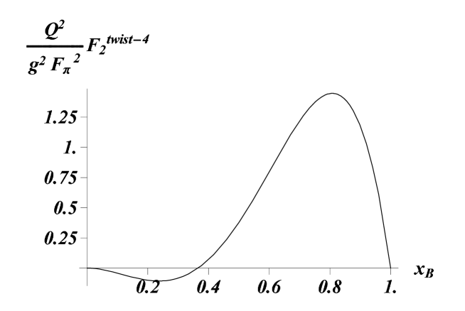
Figure 1: The result for $\frac{Q^{2}}{g^{2}F_{\pi}^{2}}F_{2}^{I=2}(x_{B})$ in the large $N_{c}$ limit for the case of the asymptotic pion distribution amplitude.

We see that function $F_{2}^{I=2}(x_{B})$ is concentrated at relatively large values of $x_{B}$. Let us note that the isospin-2 pion structure function should have at least one zero due to the general sum rule

$$\int_{0}^{1}\frac{dx_{B}}{x_{B}^{2}}\ F_{2}^{I=2}(x_{B})=0\,,$$ (30)

which directly follows from eq. (2) and holds already at finite $N_{c}$.

We have demonstrated that in the large $N_{c}$ limit the higher twist quark-antiquark correlations in mesons are expressible completely in terms of their twist-2 distribution amplitudes. This model-independent result provides an illustration of general relations between higher twist structure functions and hadron wave functions as recently discussed by S.J. Brodsky [8].

Acknowledgements
We are grateful to A. Belitsky, J. Collins, M. Franz, L.N. Lipatov, H.-Ch. Kim, V.Yu. Petrov, O.V. Teryaev, and C. Weiss for useful discussions. The work is supported in parts by DFG, BMBF, and RFBR.

References

[1]
E. V. Shuryak and A. I. Vainshtein,
Nucl. Phys. B199 (1982) 451;
Nucl. Phys. B201 (1982) 141.
[2]
R. L. Jaffe and M. Soldate,
Phys. Lett. B105 (1981) 467;
Phys. Rev. D26 (1982) 49.
[3]
M. A. Shifman, A. I. Vainshtein and V. I. Zakharov,
Sov. Phys. JETP 45 (1977) 670.
[4] R.K. Ellis, W. Furmanski, R. Petronzio, Nucl. Phys.
B212 (1983) 29.
[5]
J. Qiu and G. Sterman,
Nucl. Phys. B353 (1991) 105.
[6] G. ’t Hooft, Nucl. Phys. B72 (1974) 461.
[7] S. Capitani et al., Nucl. Phys.
B570 (2000) 393;
S. Capitani et al.,
“Four-quark operators in hadrons,” hep-lat/0010043.
[8]
S. J. Brodsky, “Dynamical higher-twist and high phenomena: A
window to quark-quark correlations in QCD,” hep-ph/0006310.