Weyl symmetric representation of hadronic flux tubes
in the dual Ginzburg-Landau theory

Abstract

Hadronic flux-tube solutions describing the mesonic and the baryonic states within the dual Ginzburg-Landau (DGL) theory are investigated by using the dual lattice formulation in the Weyl-symmetric approach. The shape of the flux tubes is determined by placement of the color-electric Dirac-string singularity treated as a connected stack of quantized plaquettes in the dual lattice formulation. The Weyl symmetric profiles of the hadronic flux tubes are obtained by using the manifestly Weyl invariant representation of the dual gauge field.

I Introduction

The investigation of the dynamics of an Abrikosov vortex in the ordinary superconductor is an important subject to understand superconductivity. Now, we encounter quite a similar situation in the study of the QCD vacuum and the hadron structure, since studies of lattice QCD in the maximally Abelian gauge [1, 2, 3] show numerical evidence of Abelian dominance [4, 5, 6] and monopole condensation [7, 8, 9, 10] for the nonperturbative vacuum of QCD. It means that the QCD vacuum can be considered as the dual superconductor [11, 12] described by the dual Ginzburg-Landau (DGL) theory [13, 14]. In this vacuum, the color-electric flux is squeezed into an almost one dimensional object like a string due to the dual Meissner effect caused by monopole condensation. The various hadronic objects like the meson and the baryon are formed with the flux tubes existing in this picture. Hence it is very important to investigate the flux-tube dynamics in the QCD vacuum.

The DGL theory can be obtained by using the Abelian projection [15]. This scheme reduces the SU($N$) gauge theory to [U(1)]^N-1 Abelian gauge theory including color-magnetic monopoles. The symmetry [U(1)]^N-1 corresponds to the maximal torus subgroup of SU($N$). Here, the dual gauge field is introduced by the Zwanziger formalism, which makes the electro-magnetic duality manifest in the presence of both electric charge and magnetic charge [16]. The summation over monopole world lines in four-dimensional space time can be rewritten as the theory of a complex scalar field which interacts with the dual gauge field [17]. Assuming monopole condensation, we finally get a Ginzburg-Landau type Lagrangian with [U(1)]² dual gauge symmetry as an effective theory of nonperturbative QCD [13, 14]. According to the fact that QCD is a SU(3) gauge theory, there appear three different types of the Abelian color charges in the DGL theory, both in the electric sector and the magnetic sector, due to the Abelian projection. The color-electric charge and the color-magnetic charge are defined in the weight vector and the root vector diagram, respectively, of the SU(3) algebra such as to satisfy the Dirac quantization condition. These charges possess the global Weyl symmetry, which is permutation invariance among color labels of these charges, so that the Weyl invariance is an important aspect of the color-singlet criterion.

In this paper, we study hadronic flux-tube solutions corresponding to mesonic and baryonic states in the [U(1)]² DGL theory, which are given by various kinds of combination of the color-electric charges. The baryonic state, which is composed of three different types of the color-electric charge, is a characteristic new element of [U(1)]² DGL theory. When we obtain the solution, we pay special attention to the Weyl symmetry, since the color-singlet state must be invariant under the Weyl transformation. This can be achieved by using the manifestly Weyl symmetric representation of the dual gauge field. We also study the usual Cartan representation with 3- and 8- basis for comparison [18].

We first start from the U(1) DGL theory (dual Abelian Higgs model [19]) in order to get acquaintance with the general features of DGL theory. The dual lattice formulation is introduced to obtain the various shapes of the flux-tube solution. In the one-potential form of the DGL Lagrangian in contrast to Zwanziger’s two-potential form, there appears a nonlocal term which leads to the string-like singularity inside the flux tube. We call this color-electric Dirac string. The lattice formulation is useful to treat the Dirac string singularity, since it is not defined on the dual lattice but on the ordinary lattice. Next, we investigate the [U(1)]² DGL theory by using a similar but extended dual lattice formulation. We discuss the various representations of the dual gauge field including the Weyl symmetric representation. Finally, we apply these formulation to systematically obtain the mesonic and the baryonic flux configurations [See, Fig. 1].

II The U(1) DGL theory (dual Abelian Higgs model)

In order to warm up for the [U(1)]² DGL theory in the next section, we start from the U(1) DGL theory with external quark sources, which is regarded to represent the SU(2) gluodynamics in the Abelian projection. In this section, we mention some essential structures of the dual lattice formulation for solving the non linear field equations for flux tubes. In the presence of both electric and magnetic charges, we have at least two forms of the Lagrangian, the Zwanziger form [16] containing electric and magnetic vector potentials and the Blagojevic and Senjanovic (BS) form [20]. Although the Zwanziger form is useful to see the duality between the electric sector and the magnetic sector, we adopt in this paper the BS form since in its one-potential form, written only in terms of the dual gauge field, the flux-tube solutions are easy to see.

A The general feature

The U(1) DGL theory is given by the Lagrangian

$${\cal L}_{\rm U(1)\;DGL}=-\frac{1}{4}{}^{*\!}F_{\mu\nu}^{2}(B,j)+\left|\left(\partial_{\mu}+i\hat{g}B_{\mu}\right)\chi\right|^{2}-\hat{\lambda}\left(|\chi|^{2}-\hat{v}^{2}\right)^{2},$$ (1)

where $B_{\mu}$ and $\chi$ are the dual gauge field and the complex scalar monopole field, respectively. The dual gauge coupling is $\hat{g}$, and $\hat{\lambda}$ characterizes the strength of monopole self interaction. The monopole condensate $\hat{v}$ determines the mass scale of the system. The dual field strength tensor ${}^{*\!}F_{\mu\nu}$ has the form

$${}^{*\!}F_{\mu\nu}(B,j)=\partial_{\mu}B_{\nu}-\partial_{\nu}B_{\mu}-\frac{1}{n\cdot\partial}\epsilon_{\mu\nu\alpha\beta}n^{\alpha}j^{\beta}.$$ (2)

Here, the nonlocal term appears as a contribution of the external quark current

$$j_{\mu}=\frac{e}{2}\bar{q}\gamma_{\mu}q,$$ (3)

where the factor $1/2$ is the weight of SU(2) algebra. Accordingly, $e/2$ becomes the Abelian color-electric charge in SU(2) gluodynamics in the Abelian projection. The nonlocal term is written more explicitly as

$$\frac{1}{n\cdot\partial}\varepsilon_{\mu\nu\alpha\beta}n^{\alpha}j^{\beta}(x)=\int d^{4}x^{\prime}\langle x|\frac{1}{n\cdot\partial}|x^{\prime}\rangle\varepsilon_{\mu\nu\alpha\beta}n^{\alpha}j^{\beta}(x^{\prime}),$$ (4)

where $\langle x|\frac{1}{n\cdot\partial}|x^{\prime}\rangle$ is the kernel which satisfies the equation

$$(n\cdot\partial)_{x}\langle x|\frac{1}{n\cdot\partial}|x^{\prime}\rangle=\delta^{(4)}(x-x^{\prime}).$$ (5)

Therefore, the solution is found to be

$$\langle x|\frac{1}{n\cdot\partial}|x^{\prime}\rangle = \left[p\theta((x-x^{\prime})\cdot n)-(1-p)\theta((x^{\prime}-x)\cdot n)\right]\delta^{(3)}(\vec{x}_{\perp}-\vec{x}^{\prime}_{\perp}).$$ (6)

Here $p$ is an arbitrary real number and $\delta^{(3)}(x)$ is the $\delta$-function defined on a three dimensional hyper-surface which has the normal vector $n_{\mu}$, so that $\vec{x}_{\perp}$ and $\vec{x}^{\prime}_{\perp}$ are three-vectors (generically not spatial) which are perpendicular to $n_{\mu}$. One finds that this nonlocal term represents the string-like singularity, known as the color-electric Dirac string. But now, there is only one type of color in U(1) DGL theory. When we extend this idea to the [U(1)]² DGL theory, we will have three types of color-electric Dirac strings.

In the one-potential form of the U(1) DGL theory, the dual gauge field includes another color-electric Dirac string attached to the color-electric charge of a quark, which is canceled by the color-electric Dirac string in the nonlocal term. In other words, the color-electric charge of the quark is defined by the cancellation of the color-electric Dirac string in the dual field tensor [21]. Usually, such a singularity is considered to come from the phase of the monopole field, which is of course possible since they are related by singular dual gauge transformation. However, when we include the quark (color-electric charge) source in the theory, it seems natural to regard that the dual gauge field $B_{\mu}$ itself has a singular part from the beginning.

It should be noted that the color-electric Dirac string is “ dual ” to the original magnetic Dirac string which is attached to a magnetic monopole in the Abelian gauge theory like QED. One may remember that the direction of a magnetic Dirac string can be varied by a singular Abelian gauge transformation, and hence, the magnetic Dirac string is unphysical in the sense that one cannot detect it. In our case, however, the symmetry which is responsible for the direction of the color-electric Dirac string is the dual gauge symmetry, achieved by a set of transformation :

$$\chi\to\chi e^{if},\quad\chi^{*}\to\chi^{*}e^{-if},\quad B_{\mu}\to B_{\mu}-\frac{1}{\hat{g}}\partial_{\mu}f,$$ (7)

$$-\frac{1}{\hat{g}}[\partial_{\mu},\partial_{\nu}]f-\frac{1}{n\cdot\partial}\varepsilon_{\mu\nu\alpha\beta}n^{\alpha}j^{\beta}\to\frac{1}{n^{\prime}\cdot\partial}\varepsilon_{\mu\nu\alpha\beta}n^{{}^{\prime}\alpha}j^{\beta},$$ (8)

where the dual gauge fixing function can be singular ($[\partial_{\mu},\partial_{\nu}]f\neq 0$). The last relation in (8) determines the new direction of the color-electric Dirac string $n_{\mu}^{\prime}$. This dual gauge symmetry would be broken by monopole condensation $\langle 0|\chi|0\rangle=\hat{v}$. This is the so-called dual Higgs mechanism, which is realized by inserting $\chi=\left(\hat{v}+\phi/\sqrt{2}\right)e^{i\eta}\;$ (where $\phi,\eta\in\Re$) into the U(1) DGL Lagrangian as

$${\cal L}_{\rm U(1)\;DGL} = -\frac{1}{4}{}^{*\!}F_{\mu\nu}^{2}(B^{\prime},j)+\frac{1}{2}m_{B}^{2}B_{\mu}^{{}^{\prime}2}+\frac{1}{2}\left[(\partial_{\mu}\phi)^{2}-m_{\chi}^{2}\phi^{2}\right]$$ (10)

$$+\hat{g}^{2}B_{\mu}^{{}^{\prime}2}\left(\sqrt{2}\hat{v}\phi+\frac{\phi^{2}}{2}\right)-\hat{\lambda}\left(\sqrt{2}\hat{v}\phi^{3}+\frac{\phi^{4}}{4}\right),$$

where the phase of the monopole field $\eta$ is absorbed into the dual gauge field as $B^{\prime}_{\mu}=B_{\mu}+\partial_{\mu}\eta/\hat{g}$, and accordingly, the dual gauge field and the monopole field acquire the masses $m_{B}\equiv\sqrt{2}\hat{g}\hat{v}$ and $m_{\chi}\equiv 2\sqrt{\hat{\lambda}}\hat{v}$, respectively. In that case, only the region where the field $\chi\approx 0$ resembles the normal phase in the dual superconductor vacuum, which means that the color-electric field can survive only near the region $\chi\approx 0$. Then, the color-electric Dirac string has a physical meaning, since the “ normal region ” follows the color-electric Dirac string so as to minimize the energy of the system forming the color-electric flux tube. It means that the shape and the size of this normal region are determined by the direction $n_{\mu}$ and length, respectively. The width of the flux tube is characterized by the inverse masses $m_{B}^{-1}$ and $m_{\chi}^{-1}$, which correspond to the penetration depth of the color-electric field and the coherence length of the monopole field, respectively. The vacuum property, namely the type of dual superconductivity, is governed by the ratio of these lengths, the so-called Ginzburg-Landau (GL) parameter

$$\hat{\kappa}\equiv\frac{m_{B}^{-1}}{m_{\chi}^{-1}}=\frac{\sqrt{2\hat{\lambda}}}{\hat{g}}.$$ (11)

Here, $\hat{\kappa}=1$ is the critical case, the so-called Bogomol’nyi limit, and the vacuum is classified into two types divided by this limit: $\hat{\kappa}<1$ belongs to the type-I vacuum and $\hat{\kappa}>1$ is the type-II vacuum. The profile functions connecting the normal phase in the center of the flux tube with the dual superconducting phase outside are classically determined by the field equations

$$\partial^{\nu}{}^{*\!}F_{\mu\nu}=-i\hat{g}\left(\chi^{*}\partial_{\mu}\chi-\chi\partial_{\mu}\chi^{*}\right)+2\hat{g}^{2}B_{\mu}\chi^{*}\chi\equiv k_{\mu},$$ (12)

$$\left(\partial_{\mu}+i\hat{g}B_{\mu}\right)^{2}\chi=-2\hat{\lambda}\chi(\chi^{*}\chi-\hat{v}^{2}),$$ (13)

where $k_{\mu}$ is the monopole supercurrent which circulates in a transition region, confining the normal phase inside the dual superconducting phase. Solving these field equations, the boundary condition are determined by the position of the color-electric Dirac string, and this information is included in the dual field strength tensor as a nonlocal term. In the following subsection, we explain the dual lattice formulation to solve such non linear equations and see how this formulation enables us to obtain various shapes of the flux-tube solutions.

B The dual lattice formulation

In order to formulate the U(1) DGL theory on the dual lattice, taking into account (3), it is convenient to write the nonlocal term as

$$\frac{1}{n\cdot\partial}\varepsilon_{\mu\nu\alpha\beta}n^{\alpha}j^{\beta}\equiv\frac{e}{2}\Sigma_{\mu\nu},$$ (14)

where $\Sigma_{\mu\nu}$ denotes the singular field strength. By using the relation (4) and (6), one finds that $\Sigma_{\mu\nu}$ satisfies

$$\int_{S}\Sigma_{\mu\nu}d\sigma^{\mu\nu}=\pm 1,$$ (15)

where $S$ is a certain surface which is pierced by the color-electric Dirac string and the sign depends on the direction of the singular flux $\Sigma_{\mu\nu}$. This is the Dirac quantization condition. Accordingly, this also leads to the flux quantization condition of the color-electric flux induced by the dual gauge field.

As long as we are interested in a three-dimensional static system, we can start from the Euclidean metric instead of the Minkowski metric. Then, the U(1) DGL Lagrangian is written as

$${\cal L}_{\rm U(1)DGL}=+\frac{1}{4}{}^{*\!}F_{\mu\nu}^{2}(B,\Sigma)+\left|\left(\partial_{\mu}+i\hat{g}B_{\mu}\right)\chi\right|^{2}+\hat{\lambda}\left(|\chi|^{2}-\hat{v}^{2}\right)^{2},$$ (16)

where

$${}^{*\!}F_{\mu\nu}(B,\Sigma)=\partial_{\mu}B_{\nu}-\partial_{\nu}B_{\mu}-\frac{e}{2}\Sigma_{\mu\nu}.$$ (17)

Now, we formulate this on the dual lattice. Let the dual gauge field be defined on links as $B_{x,\mu}$, the monopole field on sites as $\chi_{x}$, and the dual field strength tensor and the color-electric Dirac string term on plaquettes as ${}^{*\!}F_{x,\mu\nu}$ and $\Sigma_{x,\mu\nu}$. The color-electric charge and anticharge are attached to the ends of the color-electric Dirac string. We go over to dimensionless fields by the transformation :

$$B_{x,\mu}\to\frac{\hat{B}_{x,\mu}}{a\hat{g}},\quad\chi_{x}\to\hat{v}\hat{\chi}_{x},\quad\Sigma_{x,\mu\nu}\to\frac{\hat{\Sigma}_{x,\mu\nu}}{a^{2}},$$ (18)

where $a$ is dual lattice spacing, which has the dimension of length and can be reinserted when needed. Accordingly, the scale is absorbed into the definition of masses of the dual gauge field $m_{B}\equiv\sqrt{2}\hat{g}\hat{v}$, and the monopole field $m_{\chi}\equiv 2\sqrt{\hat{\lambda}}\hat{v}$. Then, the action on the dual lattice is given by

$$S=\sum_{x}\hat{\beta}\left[\frac{1}{2}\sum_{\mu<\nu}{}^{*\!}\hat{F}_{x,\mu\nu}^{2}+\frac{\hat{m}_{B}^{2}}{2}\sum_{\mu}\left|\hat{\chi}_{x}-e^{i\hat{B}_{x,\mu}}\hat{\chi}_{x+\hat{\mu}}\right|^{2}+\frac{\hat{m}_{B}^{2}\hat{m}_{\chi}^{2}}{8}\left(|\hat{\chi}_{x}|^{2}-1\right)^{2}\right],$$ (19)

where $\hat{\beta}\equiv 1/\hat{g}^{2}$, $\hat{m}_{B}\equiv m_{B}\cdot a$ and $\hat{m}_{\chi}\equiv m_{\chi}\cdot a$ [22]. The dimensionless dual field strength with the external source is given by

$${}^{*\!}\hat{F}_{x,\mu\nu}=\hat{B}_{x,\mu}+\hat{B}_{x+\hat{\mu},\nu}-\hat{B}_{x+\hat{\nu},\mu}-\hat{B}_{x,\nu}-2\pi\hat{\Sigma}_{x,\mu\nu},$$ (20)

where the relation between the color-electric charge and the color-magnetic charge, the Dirac quantization condition, $eg=4\pi$ is used. The integral form of the color-electric flux quantization condition (15) is then replaced by putting

$$\hat{\Sigma}_{x,\mu\nu}=\pm 1,$$ (21)

on just a single plaquette in the $\mu\nu$ plane. In the dual lattice formulation, the kinetic term of the monopole field is written as

$$(\partial_{\mu}+i\hat{g}B_{\mu})\chi \to \frac{\hat{v}}{a}\left(U_{x,\mu}\hat{\chi}_{x+\hat{\mu}}-\hat{\chi}_{x}\right),$$ (22)

where $U_{x,\mu}$ is a (compact) link variable,

$$U_{x,\mu}=\exp\;(ia\hat{g}B_{x,\mu})=\exp\;(i\hat{B}_{x,\mu}).$$ (23)

In the static three-dimensional system, we only need space-like links $\mu$ or $\nu=1,2,3$. Note that four-dimensional Monte Carlo simulation of U(1) DGL theory in Euclidean metric is possible if we add the time-like link contribution.

The field equation on the lattice is obtained when we formulate the cooling procedure, which aims to minimize the action (19). We require that the first derivative of the action with respect to the dual gauge field and the monopole field becomes zero. For the dual gauge field $\hat{B}_{x,i=1,2,3}$, this condition leads to

$$\frac{\partial S}{\partial\hat{B}_{x,i}}=\hat{\beta}\left({}^{*\!}\hat{F}_{x,ij}+{}^{*\!}\hat{F}_{x-\hat{j},ji}+{}^{*\!}\hat{F}_{x,ik}+{}^{*\!}\hat{F}_{x-\hat{k},ki}+m_{B}^{2}b_{x,i}^{(2)}\right)\equiv\hat{\beta}X_{x,i},$$ (24)

(25)

which corresponds to Eq.(12) in the continuum limit. Here we have defined

$$b_{x,i}^{(1)} \equiv \hat{\chi}_{x}^{R}\left(\hat{\chi}_{x+\hat{i}}^{R}\cos\hat{B}_{x,i}-\hat{\chi}_{x+\hat{i}}^{I}\sin\hat{B}_{x,i}\right)+\hat{\chi}_{x}^{I}\left(\hat{\chi}_{x+\hat{i}}^{R}\sin\hat{B}_{x,i}+\hat{\chi}_{x+\hat{i}}^{I}\cos\hat{B}_{x,i}\right),$$ (26)

$$b_{x,i}^{(2)} \equiv \hat{\chi}_{x}^{R}\left(\hat{\chi}_{x+\hat{i}}^{R}\sin\hat{B}_{x,i}+\hat{\chi}_{x+\hat{i}}^{I}\cos\hat{B}_{x,i}\right)-\hat{\chi}_{x}^{I}\left(\hat{\chi}_{x+\hat{i}}^{R}\cos\hat{B}_{x,i}-\hat{\chi}_{x+\hat{i}}^{I}\sin\hat{B}_{x,i}\right).$$ (27)

The labels $i,j,k=1,2,3$ should be taken cyclically. We find that the four terms of the dual field strength tensor ${}^{*\!}\hat{F}_{x,ij}\sim{}^{*\!}\hat{F}_{x-\hat{k},ki}$ in (25) are nothing else but the sum of plaquettes which are attached to the link at $x$ pointing into $i$-direction. The superscript of the monopole field $R,I$ denote its real and its imaginary part. The candidate value of the dual gauge potential, which locally satisfies the dual lattice field equations $X_{x,i}=0$, is obtained by a relaxation step taking into account the second derivative of the action, a la Newton and Raphson as

$$\hat{B}_{x,i}\to\hat{B}_{x,i}^{\prime} = \hat{B}_{x,i}-\left(\frac{\partial^{2}S}{\partial\hat{B}_{x,i}^{2}}\right)^{-1}\frac{\partial S}{\partial\hat{B}_{x,i}}$$ (28)

$$= \hat{B}_{x,i}-\frac{X_{x,i}}{4+\hat{m}_{B}^{2}b_{x,i}^{(1)}}.$$ (29)

For the monopole field, similarly, the local solution is given by the update

$$\hat{\chi}_{x}^{R}\to\hat{\chi}_{x}^{R\;^{\prime}} = \hat{\chi}_{x}^{R}-\frac{X_{x}^{R}}{6+\frac{1}{2}\hat{m}_{\chi}^{2}\left(\hat{\chi}_{x}^{R\;2}+\hat{\chi}_{x}^{I\;2}-1\right)}$$ (31)

$$+\frac{\hat{m}_{\chi}^{2}\hat{\chi}_{x}^{R}\left(\hat{\chi}_{x}^{R}X_{x}^{R}+\hat{\chi}_{x}^{I}X_{x}^{I}\right)}{\biggl{\{}6+\frac{1}{2}\hat{m}_{\chi}^{2}\left(\hat{\chi}_{x}^{R\;2}+\hat{\chi}_{x}^{I\;2}-1\right)\biggr{\}}\biggl{\{}6+\frac{1}{2}\hat{m}_{\chi}^{2}\left(\hat{\chi}_{x}^{R\;2}+\hat{\chi}_{x}^{I\;2}-1\right)+\hat{m}_{\chi}^{2}\left(\hat{\chi}_{x}^{R\;2}+\hat{\chi}_{x}^{I\;2}\right)\biggr{\}}},$$

$$\hat{\chi}_{x}^{I}\to\hat{\chi}_{x}^{I\;^{\prime}} = \hat{\chi}_{x}^{I}-\frac{X_{x}^{I}}{6+\frac{1}{2}\hat{m}_{\chi}^{2}\left(\hat{\chi}_{x}^{R\;2}+\hat{\chi}_{x}^{I\;2}-1\right)}$$ (34)

$$+\frac{\hat{m}_{\chi}^{2}\hat{\chi}_{x}^{I}\left(\hat{\chi}_{x}^{R}X_{x}^{R}+\hat{\chi}_{x}^{I}X_{x}^{I}\right)}{\biggl{\{}6+\frac{1}{2}\hat{m}_{\chi}^{2}\left(\hat{\chi}_{x}^{R\;2}+\hat{\chi}_{x}^{I\;2}-1\right)\biggr{\}}\biggl{\{}6+\frac{1}{2}\hat{m}_{\chi}^{2}\left(\hat{\chi}_{x}^{R\;2}+\hat{\chi}_{x}^{I\;2}-1\right)+\hat{m}_{\chi}^{2}\left(\hat{\chi}_{x}^{R\;2}+\hat{\chi}_{x}^{I\;2}\right)\biggr{\}}},$$

where

$$X_{x}^{R} = 6\hat{\chi}_{x}^{R}-\sum_{i=1}^{3}\left\{\left(\hat{\chi}_{x+\hat{i}}^{R}\cos\hat{B}_{x,i}-\hat{\chi}_{x+\hat{i}}^{I}\sin\hat{B}_{x,i}\right)+\left(\hat{\chi}_{x-\hat{i}}^{R}\cos\hat{B}_{x-\hat{i},i}+\hat{\chi}_{x-\hat{i}}^{I}\sin\hat{B}_{x-\hat{i},i}\right)\right\}$$ (37)

$$+\frac{1}{2}\hat{m}_{\chi}^{2}\hat{\chi}_{x}^{R}\left(\hat{\chi}_{x}^{R\;2}+\hat{\chi}_{x}^{I\;2}-1\right),$$

$$X_{x}^{I} = 6\hat{\chi}_{x}^{I}-\sum_{i=1}^{3}\left\{\left(\hat{\chi}_{x+\hat{i}}^{R}\sin\hat{B}_{x,i}+\hat{\chi}_{x+\hat{i}}^{I}\cos\hat{B}_{x,i}\right)+\left(\hat{\chi}_{x-\hat{i}}^{R}(-\sin\hat{B}_{x-\hat{i},i})+\hat{\chi}_{x-\hat{i}}^{I}\cos\hat{B}_{x-\hat{i},i}\right)\right\}$$ (40)

$$+\frac{1}{2}\hat{m}_{\chi}^{2}\hat{\chi}_{x}^{I}\left(\hat{\chi}_{x}^{R\;2}+\hat{\chi}_{x}^{I\;2}-1\right).$$

The dual lattice field equation for the monopole field are $X_{x}^{R}=X_{x}^{I}=0$, which corresponds to Eq. (13) in the continuum limit.

One finds that the behavior of the classical profile does not depend on the coupling $\hat{\beta}$, since this is factored out from the field equation. Hence, one can set any $\hat{\beta}$ to study the behavior of profile. At the same time, this implies that it is not necessary to specify the lattice spacing $a$. Once the masses $m_{B}$ and $m_{\chi}$ are provided in physical units, the lattice spacing $a$ is known to characterize thickness and length of the flux tube.

It is noted that when we discuss the magnitude of profiles or the classical string tension of the flux tube, $\hat{\beta}$ should be taken into account. In such case, $a$ also becomes important, since the dimensionful physical quantities are recovered by using this $a$.

C The solution

Now, the boundary condition of the dual lattice field equations becomes very easy to handle, since all we have to do is to place a set of configurations of plaquettes $\hat{\Sigma}_{x,\mu\nu}\neq 0$ which is pierced by the color-electric Dirac string in the three dimensional space. For instance, if we assume that a straight color-electric Dirac string is placed on the $z$ axis, which means that the quark and the anti-quark are placed on the $z$ axis, the only non-vanishing plaquette is $\hat{\Sigma}_{x,12}$, where $x=(0,0,x^{3})$ and $x^{3}$ belongs to the region between a quark and an anti-quark. A schematic figure is shown in Fig. 2(a), where the non-vanishing plaquettes are shaded. They form a connected stack of plaquettes dual to the color-electric Dirac string connecting $q$ and $\bar{q}$. Here, $\hat{\Sigma}_{x,\mu\nu}=+1$ $(-1)$ means that the color-electric Dirac string is regarded piercing the $\mu\nu$-plane at $x$ to $\mu\wedge\nu$ ($-\mu\wedge\nu$) direction.

In Fig. 3 we show the profiles of the color-electric field, the color-magnetic current which circulates around the flux tube, and the modulus of the monopole field. Here a $32^{3}$ dual lattice is used, and the mass parameters are taken as $\hat{\beta}=1$, $\hat{m}_{B}=\hat{m}_{\chi}=0.5$. The quark and the antiquark position are taken as $(x,y,z)=(0,0,-8)$ and $(0,0,8)$, respectively. The color-electric field is given by the space-space components of the dual field strength tensor (20), ${}^{*\!}\hat{F}_{x,ij}$ $(i,j=1,2,3)$. The color-magnetic current is minus of the last term of $X_{x,i=1,2,3}$ in (25), $-\hat{m}_{B}^{2}b_{x,i}^{(2)}$, which corresponds to $k_{\mu}$ in (12) in the continuum limit. The length of the arrows in these figures show the relative strength of fields. In the figure of the color-electric field, one can observe the Coulombic behaviors of the field at (near) the position of the quark (source) and the antiquark (sink). Here, in order to obtain the vector variables defined on sites from the color-electric fields on plaquettes and the color-magnetic currents on links, the appropriate averages like ${}^{*\!}\hat{F}^{\rm fig}_{x,ij}\equiv({}^{*\!}\hat{F}_{x,ij}+{}^{*\!}\hat{F}_{x+\hat{k},ij})/2$, where $(i,j,k:cyclic)$, etc. are associated with centers of cubes. This is also where the quark and the antiquark are located. Note that the parameter set used here is optimal for a $32^{3}$ dual lattice and intended to compare with Ref. [22], where the relation of the flux-tube profile between the classical solution of U(1) DGL theory and that of the Abelian projected SU(2) lattice gauge theory [23] is discussed.

The relation $\hat{m}_{B}=\hat{m}_{\chi}$ implies that the vacuum is at the Bogomol’nyi limit, just between type-I and type-II vacuum. The inter-quark potential is shown in Fig. 4. One finds that the slope of the linear part of the potential, which is the string tension, obeys the analytic result on the Bogomol’nyi limit, as $\sigma^{L}=2\pi\hat{v}^{2}\cdot a^{2}=\hat{\beta}\pi\hat{m}_{B}^{2}\sim 0.78$ [24, 25]. Here, the superscript “ ^L ” denotes the dimensionless string tension. Note that the force always contains a Coulomb self-energy, which corresponds to a constant term in the potential $V(R/a)$. If we choose a finer dual lattice, smaller $a$, the self energy becomes large, and accordingly, the constant takes a larger value. In such case, we could observe the fine structure of the short-distance behavior of the potential. In this paper, we only pay attention to the long distance region.

It is worth emphasizing that the dual lattice formulation presented here is also applicable to the “ bending ” flux tube [See Fig. 2(b)]. If we assume that the bending is restricted in 1-3 plane, that means that a $x^{1}$-component of the color-electric Dirac string appears, i.e. some terms $\hat{\Sigma}_{x,23}$ have non-vanishing value, $\pm 1$. In this case, the sign of this plaquette is similarly treated as discussed above. In this sense, the dual lattice formulation is quite useful to obtain various shapes of the flux-tube solutions in U(1) DGL theory numerically. In the next section, we investigate the [U(1)]² DGL theory with the similar technique. In the [U(1)]² DGL theory, there appears a flux-tube structure which includes three valence quarks corresponding to the baryonic state. In order to study such a flux configuration, we need the skill to treat the bending flux tube.

III The [U(1)]² DGL theory

In this section, we analyze the [U(1)]² DGL theory by using a similar technique as in the previous section. The main difference from the U(1) DGL theory is now that the dual gauge symmetry is extended to [U(1)]², which corresponds to Abelian projected SU(3) gluodynamics. Accordingly, there appear three different types of color-electric charge and color-magnetic charge, respectively. Among these charges, we have the global Weyl symmetry, which is permutation invariance of the color charges.

A The general feature

The [U(1)]² DGL Lagrangian in the one-potential form similar to the U(1) case is given by

$${\cal L}_{\rm[U(1)]^{2}DGL} = -\frac{1}{4}{}^{*\!}\vec{F}_{\mu\nu}^{2}(\vec{B},\vec{j})+\sum_{i=1}^{3}\left[\left|\left(\partial_{\mu}+ig\vec{\epsilon}_{i}{\cdot}\vec{B}_{\mu}\right)\chi_{i}\right|^{2}-\lambda\left(\left|\chi_{i}\right|^{2}-v^{2}\right)^{2}\right],$$ (41)

where the dual field tensor has the form

$${}^{*\!}\vec{F}_{\mu\nu}(\vec{B},\vec{j})=\partial_{\mu}\vec{B}_{\nu}-\partial_{\nu}\vec{B}_{\mu}-\frac{1}{n\cdot\partial}\varepsilon_{\mu\nu\alpha\beta}n^{\alpha}\vec{j}^{\beta}.$$ (42)

In this Lagrangian, $\vec{B}_{\mu}$ and $\chi_{i}$ denote the two-component dual gauge field and the three-component complex scalar monopole field. The interaction between quarks through the dual gauge field and with the monopole field originates from the existence of a quark current $\vec{j}_{\mu}=e\bar{q}\gamma_{\mu}\vec{H}q$ in the nonlocal term, where $\vec{H}=(T_{3},T_{8})$. Since the quark field is regarded as a fundamental representation of SU(3) group, this has a form

$$q=\left(\begin{array}[]{c}q_{1}\\ q_{2}\\ q_{3}\end{array}\right),$$ (43)

where the labels 1, 2, 3 correspond to the three types of the color-electric charge red ($R$), blue ($B$) and green ($G$). By using the relation

$$\vec{H}=(T_{3},T_{8})=\left(\begin{array}[]{ccc}\vec{w}_{1}&0&0\\ 0&\vec{w}_{2}&0\\ 0&0&\vec{w}_{3}\end{array}\right),$$ (44)

where $\vec{w}_{j}$ are the weight vectors of the SU(3) algebra,

$$\vec{w}_{1}=\left(\frac{1}{2},\frac{1}{2\sqrt{3}}\right),\quad\vec{w}_{2}=\left(-\frac{1}{2},\frac{1}{2\sqrt{3}}\right),\quad\vec{w}_{3}=\left(0,-\frac{1}{\sqrt{3}}\right),$$ (45)

we obtain an explicit form of the quark current,

$$\vec{j}_{\mu}=e\sum_{j=1}^{3}\vec{w}_{j}\;\bar{q}_{j}\gamma_{\mu}q_{j}.$$ (46)

We find that the color-electric charge is given by $e\vec{w}_{j}$. The nonlocal term can be written in the similar way as U(1) DGL theory as

$$\frac{1}{n\cdot\partial}\varepsilon_{\mu\nu\alpha\beta}n^{\alpha}\vec{j}^{\beta} = \frac{1}{n\cdot\partial}\varepsilon_{\mu\nu\alpha\beta}n^{\alpha}\cdot e\sum_{j=1}^{3}\vec{w}_{j}\;\bar{q}_{j}\gamma^{\beta}q_{j}.$$ (47)

$$= e\sum_{j=1}^{3}\vec{w}_{j}\cdot\frac{1}{n\cdot\partial}\varepsilon_{\mu\nu\alpha\beta}n^{\alpha}\bar{q}_{j}\gamma^{\beta}q_{j}$$ (48)

$$\equiv e\sum_{j=1}^{3}\vec{w}_{j}\Sigma_{j\;\mu\nu}.$$ (49)

Here, one finds that $\Sigma_{j\;\mu\nu}$ describes the color-electric Dirac string singularity attached to the color-electric charge of $e\vec{w}_{j}$, which satisfies a similar quantization condition in integral form like (15). In this case, we have

$$\int_{S}\Sigma_{j\;\mu\nu}d\sigma^{\mu\nu}=\pm 1,$$ (50)

where $S$ is a certain surface which is pierced once by the color-electric Dirac string.

The color-magnetic charge of the monopole is defined by $g\vec{\epsilon}_{i}$, where $\vec{\epsilon}_{i}$ are the root vectors of the SU(3) algebra,

$$\vec{\epsilon}_{1}=\left(-\frac{1}{2},\frac{\sqrt{3}}{2}\right),\quad\vec{\epsilon}_{2}=\left(-\frac{1}{2},-\frac{\sqrt{3}}{2}\right),\quad\vec{\epsilon}_{3}=\left(1,0\right),$$ (51)

where the labels 1, 2, 3 correspond to dual red (${}^{*\!}R$), dual blue (${}^{*\!}B$) and dual green (${}^{*\!}G$). Here, “ ^∗ ” denotes dual. Both the gauge coupling $e$ and the dual gauge coupling $g$ are related by the Dirac quantization condition $eg=4\pi$. It might be worthwhile to remember that the relation of the root vector and the weight vector of the SU(3) algebra is given by

$$\vec{\epsilon}_{i}\cdot\vec{w}_{j}=\frac{1}{2}\left(\begin{array}[]{ccc}0&1&-1\\ -1&0&1\\ 1&-1&0\end{array}\right)=\frac{1}{2}\sum_{k=1}^{3}\epsilon_{ijk}\equiv\frac{1}{2}m_{ij},$$ (55)

where $m_{ij}$ is an integer which takes 0 or $\pm 1$.

The typical scale of the [U(1)]² DGL theory is determined by taking into account the dual Higgs mechanism as the U(1) DGL theory. By inserting $\chi_{i}=\left(v+\phi_{i}/\sqrt{2}\right)e^{i\eta_{i}}$ (where $\phi_{i},\eta_{i}\in\Re$) into the [U(1)]² DGL Lagrangian (41), we get

$${\cal L}_{\rm[U(1)]^{2}\;DGL} = -\frac{1}{4}{}^{*\!}\vec{F}_{\mu\nu}^{2}(\vec{B}^{\prime},\vec{j})+\frac{1}{2}m_{B}^{2}\vec{B}_{\mu}^{{}^{\prime}2}+\sum_{i=1}^{3}\frac{1}{2}\left[(\partial_{\mu}\phi_{i})^{2}-m_{\chi}^{2}\phi_{i}^{2}\right]$$ (57)

$$+\sum_{i=1}^{3}\left[g^{2}(\vec{\epsilon}_{i}\cdot\vec{B}_{\mu}^{\prime})^{2}\left(\sqrt{2}v\phi_{i}+\frac{\phi_{i}^{2}}{2}\right)-\lambda\left(\sqrt{2}v\phi_{i}^{3}+\frac{\phi_{i}^{4}}{4}\right)\right],$$

where the phase of the monopole field $\eta_{i}$ is absorbed into the dual gauge field $\vec{B}_{\mu}^{\prime}$, as $\vec{\epsilon}_{i}\cdot\vec{B}_{\mu}^{\prime}=\vec{\epsilon}_{i}\cdot\vec{B}_{\mu}+\partial_{\mu}\eta_{i}/g$, and accordingly the dual gauge field and the monopole field acquire the masses, $m_{B}=\sqrt{3}gv$, $m_{\chi}=2\sqrt{\lambda}v$, respectively. The GL parameter is then given by

$$\kappa\equiv\frac{m_{B}^{-1}}{m_{\chi}^{-1}}=\frac{2\sqrt{\lambda}}{\sqrt{3}g}.$$ (58)

As explained in U(1) DGL theory, $\kappa=1$ is the case of special interest, the Bogomol’nyi limit [26, 27].

B Various representations of the dual gauge field

The color-electric charge of the quark is given by three components as $R$, $B$ and $G$, which is spanned by the weight vector of SU(3) algebra. The color-magnetic charge of the monopole is defined by components as ${}^{*\!}R$, ${}^{*\!}B$ and ${}^{*\!}G$, which is spanned by the root vector of SU(3) algebra. Now, we are interested in the color-singlet state corresponding to the meson and the baryon, which should be invariant under the exchange of the color charges. Hence, it is important to pay attention to the Weyl symmetry in the DGL theory. However, since the dual gauge field $\vec{B}_{\mu}$ which connects the color-electric charge and the color-magnetic charge has only two components in the sense of Cartan decomposition, and accordingly, the independent color-electric flux has two components, we cannot observe the Weyl symmetric structure in the color-electric flux tube itself. This fact makes it difficult to see the Weyl invariant structure of hadronic states. In order to investigate the Weyl symmetric structure of the flux tube in the DGL theory, it would be favorable to represent the dual gauge field in a Weyl symmetric way.

In this subsection, we write the [U(1)]² DGL Lagrangian in various representations of the dual gauge field, among which the Weyl symmetric representation of the dual gauge field is also discussed. We first pay attention to the original Cartan representation of the dual gauge field with two components. Next, we will discuss other two possible representations of the dual gauge field, the color-electric representation and the color-magnetic representation, which are achieved by spanning the dual gauge field with the weight vector and the root vector, respectively.

1 Cartan 3-8 representation

The two-component dual gauge field $\vec{B}_{\mu}$ can be written as

$$\vec{B}_{\mu}\equiv\frac{1}{g}\left(B^{3}_{\mu},\frac{B^{8}_{\mu}}{\sqrt{3}}\right).$$ (59)

The factor $\sqrt{3}$ is to make 3- and 8- components symmetric. The dual field strength tensor becomes

$${}^{*\!}\vec{F}_{\mu\nu} = \frac{1}{g}\Biggl{(}\partial_{\mu}B_{\nu}^{3}-\partial_{\nu}B_{\mu}^{3}-2\pi(\Sigma_{1\;\mu\nu}-\Sigma_{2\;\mu\nu}),$$ (61)

$$\frac{1}{\sqrt{3}}\left\{\partial_{\mu}B_{\nu}^{8}-\partial_{\nu}B_{\mu}^{8}-2\pi(\Sigma_{1\;\mu\nu}+\Sigma_{2\;\mu\nu}-2\Sigma_{3\;\mu\nu})\right\}\Biggr{)}$$

$$\equiv \frac{1}{g}\left({}^{*\!}F_{\mu\nu}^{3},\frac{{}^{*\!}F_{\mu\nu}^{8}}{\sqrt{3}}\right),$$ (62)

where we have used $eg=4\pi$ to get the factor $2\pi$ in front of $\Sigma_{j\;\mu\nu}$. The [U(1)]² DGL Lagrangian is written as

$${\cal L}_{\rm[U(1)]^{2}DGL}^{3-8} = -\frac{1}{4g^{2}}({}^{*\!}F_{\mu\nu}^{3})^{2}-\frac{1}{12g^{2}}({}^{*\!}F_{\mu\nu}^{8})^{2}$$ (66)

$$+\left|\left(\partial_{\mu}+i\frac{1}{2}\left(-B_{\mu}^{3}+B_{\mu}^{8}\right)\right)\chi_{1}\right|^{2}-\lambda\left(\left|\chi_{1}\right|^{2}-v^{2}\right)^{2}$$

$$+\left|\left(\partial_{\mu}+i\frac{1}{2}\left(-B_{\mu}^{3}-B_{\mu}^{8}\right)\right)\chi_{2}\right|^{2}-\lambda\left(\left|\chi_{2}\right|^{2}-v^{2}\right)^{2}$$

$$+\left|\left(\partial_{\mu}+iB_{\mu}^{3}\right)\chi_{3}\right|^{2}-\lambda\left(\left|\chi_{3}\right|^{2}-v^{2}\right)^{2}.$$

Note that the Lagrangian (66) is invariant under the [U(1)]² dual gauge transformation,

$$\chi_{i}\to\chi_{i}e^{if_{i}},\quad\chi^{*}_{i}\to\chi^{*}_{i}e^{-if_{i}}\quad\quad(i=1,2,3),$$ (67)

$$(B_{\mu}^{3},\;B_{\mu}^{8})\to\left(B_{\mu}^{3}-\partial_{\mu}f_{3},\;B_{\mu}^{8}-(\partial_{\mu}f_{1}-\partial_{\mu}f_{2})\right),$$ (68)

where the phases $f_{i}$ fulfill the constraint $\sum_{i=1}^{3}f_{i}=0$ [13, 14].

The field equations are given by

$$\frac{1}{g^{2}}\partial^{\nu}{}^{*\!}F_{\mu\nu}^{3} = +\frac{i}{2}\left(\chi_{1}^{*}\partial_{\mu}\chi_{1}-\chi_{1}\partial_{\mu}\chi_{1}^{*}\right)-\frac{1}{2}\left(-B_{\mu}^{3}+B_{\mu}^{8}\right)\chi_{1}^{*}\chi_{1}$$ (71)

$$+\frac{i}{2}\left(\chi_{2}^{*}\partial_{\mu}\chi_{2}-\chi_{2}\partial_{\mu}\chi_{2}^{*}\right)-\frac{1}{2}\left(-B_{\mu}^{3}-B_{\mu}^{8}\right)\chi_{2}^{*}\chi_{2}$$

$$-i\left(\chi_{3}^{*}\partial_{\mu}\chi_{3}-\chi_{3}\partial_{\mu}\chi_{3}^{*}\right)+2B_{\mu}^{3}\chi_{3}^{*}\chi_{3},$$

$$\frac{1}{3g^{2}}\partial^{\nu}{}^{*\!}F_{\mu\nu}^{8} = -\frac{i}{2}\left(\chi_{1}^{*}\partial_{\mu}\chi_{1}-\chi_{1}\partial_{\mu}\chi_{1}^{*}\right)+\frac{1}{2}\left(-B_{\mu}^{3}+B_{\mu}^{8}\right)\chi_{1}^{*}\chi_{1}$$ (73)

$$+\frac{i}{2}\left(\chi_{2}^{*}\partial_{\mu}\chi_{2}-\chi_{2}\partial_{\mu}\chi_{2}^{*}\right)-\frac{1}{2}\left(-B_{\mu}^{3}-B_{\mu}^{8}\right)\chi_{2}^{*}\chi_{2},$$

$$\left(\partial_{\mu}+\frac{i}{2}\left(-B_{\mu}^{3}+B_{\mu}^{8}\right)\right)^{2}\chi_{1} = -2\lambda\chi_{1}\left(\chi_{1}^{*}\chi_{1}-v^{2}\right),$$ (74)

$$\left(\partial_{\mu}+\frac{i}{2}\left(-B_{\mu}^{3}-B_{\mu}^{8}\right)\right)^{2}\chi_{2} = -2\lambda\chi_{2}\left(\chi_{2}^{*}\chi_{2}-v^{2}\right),$$ (75)

$$\left(\partial_{\mu}+iB_{\mu}^{3}\right)^{2}\chi_{3} = -2\lambda\chi_{3}\left(\chi_{3}^{*}\chi_{3}-v^{2}\right).$$ (76)

From these field equations, we find the boundary conditions : If ${}^{*\!}F_{\mu\nu}^{3}$ and ${}^{*\!}F_{\mu\nu}^{8}$ have a non-vanishing nonlocal term $\Sigma_{j\;\mu\nu}$, the dual gauge field $B_{\mu}^{3}$ and $B_{\mu}^{8}$ also have the singular part. At the place where the dual gauge field is singular, the monopole field is required to disappear. At large distance from the singularity, the monopole field $\chi_{i}$ approaches the vacuum expectation value $v$ and the dual gauge field asymptotically vanishes, $B_{\mu}^{3}=B_{\mu}^{8}=0$. These field equations are to be solved by using the dual lattice formulation, and one will find that these boundary conditions are realized.

2 Color-electric representation

The dual gauge field can be expressed by using the weight vector $\vec{w}_{j}$, where the label $j=1,2,3$ corresponds to the color-electric charge, $R$, $B$ and $G$. In this sense, we call this the color-electric representation of the dual gauge field, which is defined by

$$\vec{B}_{\mu}\equiv\sqrt{\frac{2}{g_{e}^{2}}}\sum_{j=1}^{3}\vec{w}_{j}B_{j\;\mu}^{e},$$ (77)

where

$$g_{e}\equiv\frac{3}{\sqrt{2}}g,\quad B_{j\;\mu}^{e}\equiv\sqrt{2}g^{e}\vec{w}_{j}\cdot\vec{B}_{\mu}.$$ (78)

Note that now the dual gauge field is written as a three-component field, however all of them are not independent since $\sum_{j=1}^{3}B_{j\;\mu}^{e}=0$. The dual field strength tensor has the form

$${}^{*\!}\vec{F}_{\mu\nu}=\sqrt{\frac{2}{g_{e}^{2}}}\sum_{j=1}^{3}\vec{w}_{j}\left(\partial_{\mu}B_{j\;\nu}^{e}-\partial_{\nu}B_{j\;\mu}^{e}-2\pi\Sigma_{j\;\mu\nu}\right),$$ (79)

where $eg=4\pi$ is used. Then, we get the Lagrangian

$${\cal L}_{\rm[U(1)]^{2}DGL}^{\rm electric} = -\frac{1}{4g_{e}^{2}}\sum_{j=1}^{3}\left({}^{*\!}F_{j\;\mu\nu}^{e}\right)^{2}$$ (81)

$$+\sum_{i=1}^{3}\left[\left|\left(\partial_{\mu}+i\frac{1}{3}\sum_{j=1}^{3}m_{ij}B_{j\;\mu}^{e}\right)\chi_{i}\right|^{2}-\lambda\left(\left|\chi_{i}\right|^{2}-v^{2}\right)^{2}\right],$$

where

$${}^{*\!}F_{j\;\mu\nu}^{e}\equiv\partial_{\mu}B_{j\;\nu}^{e}-\partial_{\nu}B_{j\;\mu}^{e}-2\pi\left(2\Sigma_{j\;\mu\nu}-\sum_{k=1}^{3}m_{jk}^{2}\Sigma_{k\;\mu\nu}\right).$$ (82)

Here, we have used the relations

$$g\vec{\epsilon}_{i}{\cdot}\vec{B}_{\mu}=g\vec{\epsilon}_{i}{\cdot}\sqrt{\frac{2}{g_{e}^{2}}}\sum_{j=1}^{3}\vec{w}_{j}B_{j\;\mu}^{e}=\frac{1}{3}\sum_{j=1}^{3}m_{ij}B_{j\;\mu}^{e},$$ (83)

$$\vec{\epsilon}_{i}=\vec{w}_{j}-\vec{w}_{k}\quad(i,j,k:cyclic).$$ (84)

Apparently, the Lagrangian (81) is invariant under the [U(1)]³ dual gauge transformation, which is defined by

$$\chi_{i}\to\chi_{i}e^{if_{i}},\quad\chi^{*}_{i}\to\chi^{*}_{i}e^{-if_{i}},$$ (85)

$$B_{j\;\mu}^{e}\to B_{j\;\mu}^{e}+\sum_{i=1}^{3}m_{ji}\partial_{\mu}f_{i},$$ (86)

where $i,j=1,2,3$. However, this does not mean an increase of the gauge degrees of freedom because of the constraint $\sum_{j=1}^{3}B_{j\;\mu}^{e}=0$.

The field equations for $j=1,2,3$ and $i=1,2,3$ are given by

$$\frac{1}{g_{e}^{2}}\partial^{\nu}{}^{*\!}F_{j\;\mu\nu}^{e}=\sum_{i=1}^{3}m_{ij}\left[-\frac{i}{3}\left(\chi_{i}^{*}\partial_{\mu}\chi_{i}-\chi_{i}\partial_{\mu}\chi_{i}^{*}\right)+2\sum_{k=1}^{3}m_{ik}B_{k\;\mu}^{e}\chi_{i}^{*}\chi_{i}\right],$$ (87)

$$\left(\partial_{\mu}+i\frac{1}{3}\sum_{j=1}^{3}m_{ij}B_{j\;\mu}^{e}\right)^{2}\chi_{i}=-2\lambda\chi_{i}(\chi_{i}^{*}\chi_{i}-v^{2}).$$ (88)

We find that each field equation has U(1) structure, apart from the matrix structure in labels $i$ and $j$. The boundary condition is given by a similar discussion as in the Cartan representation of the dual gauge field. The main difference is that the dual gauge field represented here experiences the color-electric Dirac string singularity in a Weyl symmetric way. The dual lattice formulation will make this situation clear.

3 Color-magnetic representation

The dual gauge field can also be spanned by using the root vector $\vec{\epsilon}_{i}$, where the label $i=1,2,3$ corresponds to the monopole charge, ${}^{*\!}R$, ${}^{*\!}B$ and ${}^{*\!}G$. In this sense, we call this the color-magnetic representation of the dual gauge field [27], defined by

$$\vec{B}_{\mu}\equiv\sqrt{\frac{2}{3g_{m}^{2}}}\sum_{i=1}^{3}\vec{\epsilon}_{i}B_{i\;\mu}^{m},$$ (89)

where

$$g_{m}\equiv\sqrt{\frac{3}{2}}g,\quad\quad B_{i\;\mu}^{m}\equiv\sqrt{\frac{2}{3}}g_{m}\vec{\epsilon}_{i}\cdot\vec{B}_{\mu}.$$ (90)

Note that all $B_{i\;\mu}^{m}$ are not independent since $\sum_{i=1}^{3}B_{i\;\mu}^{m}=0$. The dual field strength tensor is written as

$${}^{*\!}\vec{F}_{\mu\nu}=\sqrt{\frac{2}{3g_{m}^{2}}}\sum_{i=1}^{3}\vec{\epsilon}_{i}\left(\partial_{\mu}B_{i\;\nu}^{m}-\partial_{\nu}B_{i\;\mu}^{m}-2\pi\sum_{j=1}^{3}m_{ij}\Sigma_{j\;\mu\nu}\right),$$ (91)

where we use $eg=4\pi$. Hence, the Lagrangian with the color-magnetic representation of the dual gauge field is given by

$${\cal L}_{\rm[U(1)]^{2}DGL}^{\rm magnetic} = \sum_{i=1}^{3}\Biggl{[}-\frac{1}{4g_{m}^{2}}\left({}^{*\!}F_{i\;\mu\nu}^{m}\right)^{2}+\left|\left(\partial_{\mu}+iB_{i\;\mu}^{m}\right)\chi_{i}\right|^{2}-\lambda\left(\left|\chi_{i}\right|^{2}-v^{2}\right)^{2}\Biggr{]},$$ (92)

where

$${}^{*\!}F_{i\;\mu\nu}^{m}\equiv\partial_{\mu}B_{i\;\nu}^{m}-\partial_{\nu}B_{i\;\mu}^{m}-2\pi\sum_{j=1}^{3}m_{ij}\Sigma_{j\;\mu\nu}.$$ (93)

Here, we have used the relations

$$\vec{w}_{i}=-\frac{1}{3}\left(\vec{\epsilon}_{j}-\vec{\epsilon}_{k}\right)\quad(i,j,k:cyclic).$$ (94)

Since the Lagrangian (92) has a quite similar form as the U(1) DGL theory, except for the labels $i$ and $j$, one finds that the dual gauge symmetry becomes very easy to observe,

$$\chi_{i}\to\chi_{i}e^{if_{i}},\quad\chi^{*}_{i}\to\chi^{*}_{i}e^{-if_{i}},\quad B_{i\;\mu}^{m}\to B_{i\;\mu}^{m}-\partial_{\mu}f_{i}\quad\quad(i=1,2,3),$$ (95)

and accordingly the Lagrangian (92) has the extended dual gauge symmetry [U(1)]³ with a constraint $\sum_{i=1}^{3}B_{i\;\mu}^{m}=0$. This is the same as in the color-electric representation of the dual gauge field.

The field equations for $i=1,2,3$ have the form

$$\frac{1}{g_{m}^{2}}\partial^{\nu}{}^{*\!}F_{i\;\mu\nu}^{m}=-i\left(\chi_{i}^{*}\partial_{\mu}\chi_{i}-\chi_{i}\partial_{\mu}\chi_{i}^{*}\right)+2B_{i\;\mu}^{m}\chi_{i}^{*}\chi_{i},$$ (96)

$$\left(\partial_{\mu}+iB_{i\;\mu}^{m}\right)^{2}\chi_{i}=-2\lambda\chi_{i}(\chi_{i}^{*}\chi_{i}-v^{2}),$$ (97)

which is exactly the same as the field equation in the U(1) DGL theory, replicated with respect to the index $i$. In this sense, the boundary conditions can be taken similarly as the U(1) case. Therefore, the color-magnetic representation of the dual gauge field is particularly simple as compared with other representations.

C The solution

In order to solve the field equation with various representations of the dual gauge field, we adopt the dual lattice formulation with the U(1) DGL theory, but extended to more degrees of freedom. In this subsection, we first investigate the mesonic flux tube, and next the baryonic flux tube. We use the words “ mesonic ” or “ baryonic ” to distinguish the real color-singlet hadron from the classical state that we deal with in this paper. For instance, if we want to obtain real meson or baryon state, we need to consider the quantum state given by

$$|meson\rangle = \frac{1}{\sqrt{3}}\left(|R\bar{R}\rangle+|B\bar{B}\rangle+|G\bar{G}\rangle\right),$$ (98)

$$|baryon\rangle = \frac{1}{\sqrt{6}}\left(|RBG\rangle+|BGR\rangle+|GRB\rangle-|RGB\rangle-|GBR\rangle-|BRG\rangle\right),$$ (99)

where $R\bar{R}$ denotes $R-\bar{R}$ flux tube, and so forth. In the classical solution, we can only treat a piece of these states. However, even then it is necessary to pay attention to the Weyl symmetry, since all states can be reduced to the same classical state for the meson and the baryon, respectively.

1 Mesonic flux tube ($q$-$\bar{q}$ system)

Since the three types of the color-electric charge are represented by non-vanishing plaquettes $\hat{\Sigma}_{x,1\;\mu\nu}$, $\hat{\Sigma}_{x,2\;\mu\nu}$ and $\hat{\Sigma}_{x,3\;\mu\nu}$, the mesonic state corresponding to $|R\bar{R}\rangle$, $|B\bar{B}\rangle$ and $|G\bar{G}\rangle$ are given by some stacks of connected plaquettes of each color. For example, if we want to consider the straight $R-\bar{R}$ flux-tube system, all we have to do is to put only one of the color-electric Dirac string plaquette $\hat{\Sigma}_{x,1\;\mu\nu}\neq 0$ like Fig. 2(a), whereas $\hat{\Sigma}_{x,2\;\mu\nu}=\hat{\Sigma}_{x,3\;\mu\nu}=0$ for all over the three dimensional space. For the $B-\bar{B}$ flux-tube system, we set $\hat{\Sigma}_{x,2\;\mu\nu}\neq 0$ and $\hat{\Sigma}_{x,3\;\mu\nu}=\hat{\Sigma}_{x,1\;\mu\nu}=0$, for the $G-\bar{G}$ flux-tube system, $\hat{\Sigma}_{x,3\;\mu\nu}\neq 0$ and $\hat{\Sigma}_{x,1\;\mu\nu}=\hat{\Sigma}_{x,2\;\mu\nu}=0$.

In Figs. 5-10, we show the profiles of the color-electric field and corresponding monopole current of $R-\bar{R}$, $B-\bar{B}$, and $G-\bar{G}$ flux-tube system for various representation of the dual gauge field, the Cartan representation, the color-electric representation, and the color-magnetic representation, respectively. We find that the last two representations enable us to see the Weyl symmetric structure of the flux tube. The Dirac string structures in the dual gauge field with various representations is summarized schematically in Table. 1.

The profile of the monopole field is shown in Fig. 11. One finds that this does not depend on the choice of the representation of the dual gauge field, since the monopole field is defined on the SU(3) root vector. That is the reason why this distribution is similar to the color-electric field in the color-magnetic representation of the dual gauge field. The inter-quark potential is shown in Fig. 12, which, of course, does not depend on the representation. The parameter set used here is the same as in the U(1) case. We took $\beta\equiv 1/g^{2}=1$, $\hat{m}_{B}=\hat{m}_{\chi}=0.5$. This set is simply to see the behavior of the profiles and to compare the string tension of the potential with the analytical value in the Bogomol’nyi limit, $\sigma^{L}=4\pi v^{2}\cdot a^{2}=4\beta\pi\hat{m}_{B}^{2}/3$ [26, 27]. One finds that the analytical string tension is reproduced by the numerical potential in Fig. 12. In order to get quantitatively realistic results, we need more information about the parameter set of U(1)² DGL theory from QCD.

It is worth noting that in the mesonic case, we can reduce the [U(1)]² DGL theory to the U(1) DGL theory [28]. Let us see this in the $R-\bar{R}$ system with the Cartan representation of the dual gauge field, as an example. Other systems and other representations can be treated similarly. Here, we already know the profiles of the color-electric flux tube and the contribution of the dual gauge field and the monopole field as shown in Figs. 5 and 11. Thus, one can take $B_{\mu}^{3}=B_{\mu}^{8}\equiv B_{\mu}$ and $\chi_{1}=v$, $\chi_{2}\equiv\chi^{*}$, $\chi_{3}\equiv\chi$. The [U(1)]² DGL Lagrangian (66) is reduced to the form,

$${\cal L}_{\rm[U(1)]^{2}DGL}^{3-8} = -\frac{1}{3g^{2}}\left(\partial_{\mu}B_{\nu}-\partial_{\nu}B_{\mu}-2\pi\Sigma_{1\;\mu\nu}\right)^{2}$$ (101)

$$+2\left[\left|\left(\partial_{\mu}+iB_{\mu}\right)\chi\right|^{2}-\lambda\left(\left|\chi\right|^{2}-v^{2}\right)^{2}\right].$$

The redefinitions of the couplings and the fields

$$g\equiv\frac{2}{\sqrt{3}}\hat{g},\quad\lambda\equiv 2\hat{\lambda},\quad v\equiv\frac{1}{\sqrt{2}}\hat{v},\quad B_{\mu}\to\hat{g}B_{\mu},\quad\chi\to\frac{\chi}{\sqrt{2}},\quad$$ (102)

lead to the Lagrangian of U(1) DGL theory as is given in (1).

2 Baryonic flux tube ($q$-$q$-$q$ system)

We solve the field equations in the presence of three types of the color-electric charges. Since these color-electric charges are defined in the weight vector diagram of SU(3) algebra, and the color-electric Dirac strings which are attached to these charges carry the same quantity, respectively, these Dirac strings can join at a certain point to cancel each other ($\sum_{j=1}^{3}e\vec{w}_{j}=0$), which we call a junction. Here, we consider the simple case that the three types of the color-electric charge are placed on the corners of a regular triangle. The non-vanishing plaquettes $\hat{\Sigma}_{x,1\;\mu\nu}$, $\hat{\Sigma}_{x,2\;\mu\nu}$ and $\hat{\Sigma}_{x,3\;\mu\nu}$ are properly included so as to minimize the length of the color-electric Dirac string, which corresponds to the energy minimization condition. Then, the position of the junction is given by the Fermat point [18]. As a result, we get a typical $Y$-shaped flux-tube object in U(1)² DGL theory, i.e. the baryonic flux tube.

In Figs. 13-15, we show the profiles of the color-electric field corresponding to the Cartan, the color-electric, and the color-magnetic representations of the dual gauge field. The Weyl symmetric structure can be observed in the last two representations. The monopole field does not depend on which representation is chosen, for the same reason as in the discussion of the mesonic flux tube, which is shown in Fig. 16. One finds that all of these profiles faithfully reflect the structure of the color-electric Dirac string. The potential is obtained analogously to the mesonic system, which is shown in Fig. 17. Here, parametrizing the potential of the linear part as

$$V(\mbox{\boldmath$x$}_{1},\mbox{\boldmath$x$}_{2},\mbox{\boldmath$x$}_{3})\sim\sigma^{L}\sum_{i=1}^{3}|\mbox{\boldmath$x$}_{i}-\mbox{\boldmath$x$}_{J}|,$$ (103)

where $\mbox{\boldmath$x$}_{i}$ and $\mbox{\boldmath$x$}_{J}$ denote the position of the quarks and of the junction on the dual lattice, respectively, we can extract the string tension $\sigma^{L}$. One finds that this is almost reproduced by the analytical one, since $\sigma^{L}\sim 1.0\sim 4\beta\pi\hat{m}_{B}^{2}/3$. It is interesting to note that while each profile of the color-electric field in the color-electric representation has similar form to the 8-flux in the Cartan representation, the color-electric field in the color-magnetic representation provides the 3-flux type structure. It is, of course, possible to study the energy and the field distribution corresponding to different shapes of baryonic flux tube in a static configuration.

IV Summary and discussion

We have studied the classical flux-tube solutions for the mesonic and the baryonic states within the dual Ginzburg-Landau (DGL) theory by using the dual lattice formulation in the Weyl symmetric approach. The color-electric Dirac string singularity, which determines the filament core inside the flux tube, has been treated as a connected stack of quantized plaquettes which lead to the phase $\pm 2\pi$ in the dual lattice formulation. This formulation is flexible to reproduce various shapes of the flux tube just by putting the quantized plaquettes which are pierced by a color-electric Dirac string of any form. We have found that the manifestly Weyl symmetric approach, in particular, the color-magnetic representation of the dual gauge field is the most convenient one to investigate flux-tube solutions in the [U(1)]² DGL theory, since this gives a quite similar form with the U(1) case [27].

In this paper we have concentrated on formulating a simple method to investigate the qualitative properties of the classical flux-tube solution in the U(1) and [U(1)]² DGL theory. This work can be extended to the study of the flux tube in the quantized DGL theory by using the Monte Carlo method in four dimensional Euclidean space time. Then, also the effect of string fluctuations becomes a possible topic of investigation. Even without string fluctuations, we can discuss more quantitative properties of the hadronic flux tubes, based on a quantum DGL theory. This is under preparation. The application of this formulation to the flux-tube ring solution as the glueball state [29] is also interesting.

A crucial criterion for a viable confinement mechanism is the ability to reproduce the Casimir scaling of the forces at intermediate distances between static charges in different representation, $F_{R_{i}}/F_{R_{j}}=C_{2}(R_{i})/C_{2}(R_{j})$ with $C_{2}$ as the eigenvalue of the quadratic Casimir operator $\lambda_{j}^{2}$ in the representations $R_{i}$ and $R_{j}$, respectively. For the ratio of adjoint to fundamental charges in SU(3) gauge theory, this would give $\sigma_{\mathrm{a}dj}/\sigma_{\mathrm{f}und}=9/4$. Casimir scaling is in the discussion since the first lattice indications for it appeared in the eighties [30], and at that time it was challenging for the bag model [31]. Enhanced attention recently, due to the lively discussion of competing confinement mechanisms, in Ref. [32] the string tensions of the fundamental and the adjoint representations were computed and the ratio came out to be nearly 2, which was close to 9/4. On the other hand, in Ref. [33] they have studied the ratio of entire potentials including Coulomb and constant terms in addition to the linear term and the ratio turns out to be very close to 9/4. All detailed and microscopic mechanisms of confinement find it hard to explain this observation, while it is more natural from the point of view of the semi-phenomenological Stochastic Vacuum Model [34].

Discussing the Abelian projection in terms of $\lambda_{3}$ and $\lambda_{8}$ would suggest to evaluate $\sigma_{\mathrm{a}dj}/\sigma_{\mathrm{f}und}$ with diagonal gluons only, giving a ratio 3. This makes it hard to understand why Casimir scaling should hold in Abelian projected gluodynamics. Considering the DGL theory just at a phenomenological level, it would be sufficient to restrict it exclusively to mesonic, baryonic, glueball and perhaps to exotic states, and it would be inappropriate to apply it to the so-called gluelump bound states made of infinitely heavy adjoint charges. However, because of the current interest, it might be amusing to consider briefly how this kind of string would be represented within the DGL theory. Although this theory, as an effective theory of gluodynamics with external charges, is constructed referring to Abelian projection, we are free to look at the Casimir problem afresh.

In fact, the DGL theory is rather promising to discuss the Casimir scaling problem without extra effort. To see this, we recall that the DGL theory represents the mesonic string as degenerate $R-\bar{R}$, $B-\bar{B}$ and $G-\bar{G}$ colored states. In the same spirit it is natural to represent gluelump strings as stretching out between pairs of adjoint charges, each of them being made out of quark and antiquark as $B\bar{G}-\bar{B}G$, $G\bar{R}-\bar{G}R$, and $R\bar{B}-\bar{R}B$ states. Thus, it is rather a string formed by two pairs with their respective Dirac strings superposed. In the Bogomol’nyi limit one directly gets the ratio $\sigma_{\mathrm{a}dj}/\sigma_{\mathrm{f}und}$ using the manifest Weyl invariant formulation of the DGL theory [27]. In this limiting case the ratio is equal to 2, reflecting the presence of two independent color-electric Dirac strings inside the adjoint flux tube. Entering the type-II dual superconductor parameter range, the ratio will increase, while decreasing towards the type-I region. Our studies show that the ratio of string tensions depends only on the ratio between dual vector and monopole mass, via $\kappa=m_{\chi}/m_{B}$. It has been conjectured that the ratio 9/4 is reproduced in a certain type-II vacuum.

TABLE I.: The color-electric Dirac string structure in the dual gauge field in $q$-$\bar{q}$ system for various representations (for Figs. 5-11) is schematically summarized. Here, $\uparrow$ and $\downarrow$ correspond to the one Dirac string singularity. If we circulate around these singularities as counter-clockwise way, they lead to the phase $+2\pi$ and $-2\pi$, respectively. Notice that $\Uparrow=2\times\uparrow$ and $\Downarrow=2\times\downarrow$.

	3-8 basis			electric basis				magnetic basis
	$B_{\mu}^{3}$	$B_{\mu}^{8}$		$B_{1\;\mu}^{e}$	$B_{2\;\mu}^{e}$	$B_{3\;\mu}^{e}$		$B_{1\;\mu}^{m}$	$B_{2\;\mu}^{m}$	$B_{3\;\mu}^{m}$
$R-\bar{R}$	$\downarrow_{c}$	$\downarrow_{c}$		$\Downarrow_{e}$	$\uparrow_{e}$	$\uparrow_{e}$		$0$	$\uparrow_{m}$	$\downarrow_{m}$
$B-\bar{B}$	$\uparrow_{c}$	$\downarrow_{c}$		$\uparrow_{e}$	$\Downarrow_{e}$	$\uparrow_{e}$		$\downarrow_{m}$	$0$	$\uparrow_{m}$
$G-\bar{G}$	$0$	$\Uparrow_{c}$		$\uparrow_{e}$	$\uparrow_{e}$	$\Downarrow_{e}$		$\uparrow_{m}$	$\downarrow_{m}$	$0$

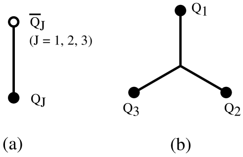
FIG. 1.: The possible combinations of the color-electric charge in the hadronic flux tubes, corresponding to (a) the meson and (b) the baryon.

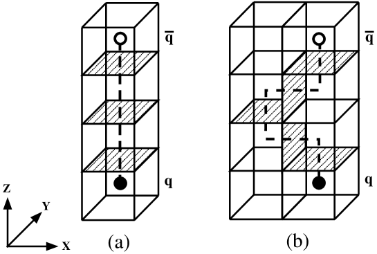
FIG. 2.: The color-electric Dirac string dual to singular plaquettes (shaded) ending in external charges.

FIG. 3.: The profile of the color-electric field in the $x$-$z$ plane at $y=0$ (left), the color-magnetic current in the $x$-$y$ plane at $z=0$ (right-upper), and the monopole field in the $x$-$z$ plane at $y=0$ (right-lower) of the mesonic flux tube in the U(1) DGL theory. The quark and the antiquark are placed at $(x,y,z)=(0,0,-8)$ and $(0,0,8)$, respectively.

FIG. 4.: The quark-antiquark potential in the U(1) DGL theory, where $R/a$ denotes the $q$-$\bar{q}$ distance. The parameter set is taken as $\hat{\beta}=1$, $\hat{m}_{B}=\hat{m}_{\chi}=0.5$.

FIG. 5.: The profiles of the color-electric field in the Cartan representation for 3- (left) and 8- (right) components in the $R-\bar{R}$ (upper), the $B-\bar{B}$ (middle), and the $G-\bar{G}$ (lower) systems in the $x$-$z$ plane at $y=0$. The quark and the antiquark are placed at $(x,y,z)=(0,0,-10)$ and $(0,0,10)$, respectively.

FIG. 6.: The profiles of the color-magnetic current in the Cartan representation for 3- (left) and 8- (right) components in the $R-\bar{R}$ (upper), the $B-\bar{B}$ (middle), and the $G-\bar{G}$ (lower) systems in the $x$-$y$ plane at $z=0$. The quark and the antiquark are placed at $(x,y,z)=(0,0,-10)$ and $(0,0,10)$, respectively.

FIG. 7.: The profiles of the color-electric field in the color-electric representation, expressed on the weight vectors of the SU(3) algebra, $\vec{w}_{1}$ (left), $\vec{w}_{2}$ (center), and $\vec{w}_{3}$ (right) in the $R-\bar{R}$ (upper), the $B-\bar{B}$ (middle), and the $G-\bar{G}$ (lower) systems in the $x$-$z$ plane at $y=0$. The quark and the antiquark are placed at $(x,y,z)=(0,0,-10)$ and $(0,0,10)$, respectively.

FIG. 8.: The profiles of the color-magnetic current in the color-electric representation, expressed on the weight vectors of the SU(3) algebra, $\vec{w}_{1}$ (left), $\vec{w}_{2}$ (center), and $\vec{w}_{3}$ (right) in the $R-\bar{R}$ (upper), the $B-\bar{B}$ (middle), and the $G-\bar{G}$ (lower) systems in the $x$-$y$ plane at $z=0$. The quark and the antiquark are placed at $(x,y,z)=(0,0,-10)$ and $(0,0,10)$, respectively.

FIG. 9.: The profiles of the color-electric field in the color-magnetic representation, expressed on the root vectors of the SU(3) algebra, $\vec{\epsilon}_{1}$ (left), $\vec{\epsilon}_{2}$ (center), and $\vec{\epsilon}_{3}$ (right) in the $R-\bar{R}$ (upper), the $B-\bar{B}$ (middle), and the $G-\bar{G}$ (lower) systems in the $x$-$z$ plane at $y=0$. The quark and the antiquark are placed at $(x,y,z)=(0,0,-10)$ and $(0,0,10)$, respectively.

FIG. 10.: The profiles of the color-magnetic current in the color-magnetic representation, expressed on the root vectors of the SU(3) algebra, $\vec{\epsilon}_{1}$ (left), $\vec{\epsilon}_{2}$ (center), and $\vec{\epsilon}_{3}$ (right) in the $R-\bar{R}$ (upper), the $B-\bar{B}$ (middle), and the $G-\bar{G}$ (lower) systems in the $x$-$y$ plane at $z=0$. The quark and the antiquark are placed at $(x,y,z)=(0,0,-10)$ and $(0,0,10)$, respectively.

FIG. 11.: The profiles of the monopole field of $|\chi_{1}|$ (left), $|\chi_{2}|$ (center), and $|\chi_{3}|$ (right) in the $R-\bar{R}$ (upper), the $B-\bar{B}$ (middle), and the $G-\bar{G}$ (lower) systems in the $x$-$z$ plane at $y=0$. The quark and the antiquark are placed at $(x,y,z)=(0,0,-10)$ and $(0,0,10)$, respectively.

FIG. 12.: The quark-antiquark potential in the [U(1)]² DGL theory, where $R/a$ denotes the $q$-$\bar{q}$ distance. The parameter set is taken as $\beta=1$, $\hat{m}_{B}=\hat{m}_{\chi}=0.5$.

FIG. 13.: The profiles of the color-electric field in the Cartan representation for 3- (upper) and 8- (lower) components in the baryonic flux tube in the $x$-$z$ plane at $y=0$. The junction and the quarks are located at $(x,y,z)=(0,0,0)$, and $R(0,0,9)$, $B(9,0,-5)$, $G(-9,0,-5)$, respectively.

FIG. 14.: The profiles of the color-electric field in the color-electric representation, expressed on the weight vectors of the SU(3) algebra, $\vec{w}_{1}$ (upper), $\vec{w}_{2}$ (middle), and $\vec{w}_{3}$ (lower) in the baryonic flux-tube system in the $x$-$z$ plane at $y=0$. The junction and the quarks are located at $(x,y,z)=(0,0,0)$, and $R(0,0,9)$, $B(9,0,-5)$, $G(-9,0,-5)$, respectively.

FIG. 15.: The profiles of the color-electric field in the color-magnetic representation, expressed on the root vectors of the SU(3) algebra, $\vec{\epsilon}_{1}$ (upper), $\vec{\epsilon}_{2}$ (middle), and $\vec{\epsilon}_{3}$ (lower) in the baryonic flux-tube system in the $x$-$z$ plane at $y=0$. The junction and the quarks are located at $(x,y,z)=(0,0,0)$, and $R(0,0,9)$, $B(9,0,-5)$, $G(-9,0,-5)$, respectively.

FIG. 16.: The profiles of the Higgs field of $|\chi_{1}|$ (upper), $|\chi_{2}|$ (middle), and $|\chi_{3}|$ (lower) in the baryonic flux-tube system in the $x$-$z$ plane at $y=0$. The junction and the quarks are located at $(x,y,z)=(0,0,0)$, and $R(0,0,9)$, $B(9,0,-5)$, $G(-9,0,-5)$, respectively.

FIG. 17.: The three-quark potential in the [U(1)]² DGL theory, where $R_{i}=|\mbox{\boldmath$x$}_{i}-\mbox{\boldmath$x$}_{J}|$. The parameter set is taken as $\beta=1$, $\hat{m}_{B}=\hat{m}_{\chi}=0.5$.

REFERENCES

• [1] A. S. Kronfeld, G. Schierholz, and U.-J. Wiese, Nucl. Phys. B293, 461 (1987).
• [2] F. Brandstaeter, U.-J. Wiese, and G. Schierholz, Phys. Lett. B272, 319 (1991).
• [3] V. G. Bornyakov, E.-M. Ilgenfritz, M. L. Laursen, V. K. Mitrjushkin, M. Müller-Preussker, A. J. van der Sijs and A. M. Zadorozhnyi, Phys. Lett. B261, 116 (1991).
• [4] T. Suzuki and I. Yotsuyanagi, Phys. Rev. D42, 4257 (1990).
• [5] G. S. Bali, V. Bornyakov, M. Müller-Preussker, and K. Schilling, Phys. Rev. D54, 2863 (1996).
• [6] K. Amemiya and H. Suganuma, Phys. Rev. D60, 114509 (1999).
• [7] T. L. Ivanenko, A. V. Pochinsky, and M. I. Polikarpov, Nucl. Phys. Proc. Suppl. 30, 565 (1993).
• [8] H. Shiba and T. Suzuki, Phys. Lett. B351, 519 (1995); N. Arasaki, S. Ejiri, S. Kitahara, Y. Matsubara, and T. Suzuki, ibid. B395, 275 (1997).
• [9] L. D. Debbio, A. D. Giacomo, G. Paffuti, and P. Pieri, Phys. Lett. B355, 255 (1995).
• [10] M. N. Chernodub, M. I. Polikarpov, and A. I. Veselov, Phys. Lett. B399, 267 (1997).
• [11] Y. Nambu, Phys. Rev. D10, 4262 (1974).
• [12] S. Mandelstam, Phys. Rept. 23C, 245 (1976).
• [13] T. Suzuki, Prog. Theor. Phys. 80, 929 (1988); S. Maedan and T. Suzuki, ibid. 81, 229 (1989).
• [14] H. Suganuma, S. Sasaki, and H. Toki, Nucl. Phys. B435, 207 (1995);
S. Sasaki, H. Suganuma, and H. Toki, Prog. Theor. Phys. 94, 373 (1995).
• [15] G. ’t Hooft, Nucl. Phys. B190, 455 (1981).
• [16] D. Zwanziger, Phys. Rev. D3, 880 (1971).
• [17] K. Bardakci and S. Samuel, Phys. Rev. D18, 2849 (1978).
• [18] S. Kamizawa, Y. Matsubara, H. Shiba, and T. Suzuki, Nucl. Phys. B389, 563 (1993).
• [19] H. B. Nielsen and P. Olesen, Nucl. Phys. B61, 45 (1973).
• [20] M. Blagojevic and P. Senjanovic, Nucl. Phys. B161, 112 (1979).
• [21] J. S. Ball and A. Caticha, Phys. Rev. D37, 524 (1988).
• [22] F. V. Gubarev, E.-M. Ilgenfritz, M. I. Polikarpov, and T. Suzuki, Phys. Lett. B468, 134 (1999).
• [23] G. S. Bali, C. Schlichter, and K. Schilling, Prog. Theor. Phys. Suppl. 131, 645 (1998).
• [24] E. B. Bogomol’nyi, Sov. J. Nucl. Phys. 24, 449 (1976).
• [25] H. J. de Vega and F. A. Schaposnik, Phys. Rev. D14, 1100 (1976).
• [26] M. N. Chernodub, Phys. Lett. B474, 73 (2000).
• [27] Y. Koma and H. Toki, Phys. Rev. D62, 054027 (2000).
• [28] H. Ichie, H. Suganuma, and H. Toki, Phys. Rev. D54, 3382 (1996);
H. Monden, H. Suganuma, H. Ichie, and H. Toki, Phys. Rev. C57, 2564 (1998).
• [29] Y. Koma, H. Suganuma, and H. Toki, Phys. Rev. D60, 074024 (1999).
• [30] C. Bernard, Nucl. Phys. B219, 341 (1983); J. Ambjorn, P. Olesen, and C. Peterson, Nucl. Phys. B240, 189 (1984).
• [31] T. H. Hansson, Phys. Lett. B166, 343 (1986).
• [32] S. Deldar, Phys. Rev. D62, 034509 (2000).
• [33] G. S. Bali, Phys. Rev. D62, 114503 (2000).
• [34] V. I. Shevchenko and Yu. A. Simonov, Phys. Rev. Lett. 85, 1811 (2000).