Jisuke Kubo and Masanori Nunami

Institute for Theoretical Physics, Kanazawa University, Kanazawa 920-1192, Japan

Abstract

Assuming that the recent result obtained from the Monte Carlo simulations on the nonperturbative existence of the pure $SU(2)$ Yang-Mills theory in five dimensions can be applied to a more general class of higher-dimensional gauge theories , we derive the conditions imposed by the nontriviality requirement on the theories. We find that the supersymmetric grand unified theories with extra dimensions prefer a large value ($\mathrel{\mathchoice{\vbox{\offinterlineskip\halign{$\m@th\displaystyle\hfil#\hfil$\cr>\crcr\sim\crcr} }}{\vbox{\offinterlineskip\halign{$\m@th\textstyle\hfil#\hfil$\cr>\crcr\sim\crcr} }}{\vbox{\offinterlineskip\halign{$\m@th\scriptstyle\hfil#\hfil$\cr>\crcr\sim\crcr} }}{\vbox{\offinterlineskip\halign{$\m@th\scriptscriptstyle\hfil#\hfil$\cr>\crcr\sim\crcr} }}}2$) of $\tan\beta$ of the minimal supersymmetric standard model, in accord with today’s possible observation of the Higgs particle at LEP2.

PACS number: 11.10.Hi, 11.10.Kk, 12.10.Dm, 12.60.Jv

1 Introduction

In recent years a variety of theories having large extra space-time dimensions have been considered [1, 2, 3, 4, 5, 6, 7]. It has been found that certain theoretical problems such as the unification of the fundamental forces and the hierarchy problem may be solved by introducing large extra dimensions (see Ref. [8, 9] for review). So far it is only a theoretical speculation that we live in more than four space-time dimensions, and experimental indications for the existence of extra dimensions are currently searched [8, 10].

It is widely believed that any interacting gauge theory in more than four dimensions, being perturbatively unrenormalizable, is a cutoff theory, and that for a certain range of energy scale it can be an effective theory of a more fundamental theory such as string theory. Is it possible to control the quantum corrections in gauge theories in more than four dimensions? Is it ensured that the massive Kaluza-Klein excitations below the compactification scale really decouple so that its effective theory below that scale becomes a four-dimensional renormalizable theory? How can we answer these questions? The investigation of the nonperturbative existence of gauge theories in higher dimensions is, therefore, not only an academic problem, but also a fundamental problem if the fundamental theory of particle physics is formulated in more than four dimensions. Recently, the pure $SU(2)$ lattice gauge theory in five dimensions has been investigated [11], where the extra dimension is assumed to be compactified on a circle with the radius of $R$. It has been found there that the scaling behavior of the Creutz ratio measured in the four-dimensional subspace indicates that the compactified theory with a nonvanishing string tension can exist nonperturbatively. That is, the investigation indicates that the theory is a cutoff-free theory. Interestingly, this observation is consistent with the existence of the nontrivial ultraviolet fixed point that can be found analytically in the $\epsilon$-expansion method [12].

It is well conceivable that not only the pure $SU(2)$ Yang-Mills theory in five dimensions can exist nonperturbatively, but also a more general class of higher-dimensional Yang-Mills theories containing bosonic and fermionic matter fields in various representations. Unfortunately, because of the lack of computer power, these investigations based on lattice gauge theories are limited, and phenomenologically interesting higher-dimensional unified gauge models will not be accessible within the framework of lattice gauge theory in near future. We therefore assume that the fact [11] that the lattice $\beta$ function of the gauge coupling can be well approximated by the one-loop form can be extended to other cases, and that the existence of an ultraviolet fixed point can be investigated on the basis of the one-loop $\beta$ functions. In doing so we would like to derive the conditions imposed by the requirement of the nontriviality of the higher-dimensional unified gauge theories. We expect phenomenological consequences from this requirement, as the upper bound of the Higgs mass of the standard model (SM) can be obtained from the nontriviality requirement of the model [13].

In Sect. II we start by summarizing the results from the Monte Carlo simulations in the pure $SU(2)$ Yang-Mills theory in five dimensions to make clear our assumptions about the nontriviality of a more general class of higher-dimensional Yang-Mills theories. In Sect III we will derive the conditions for a supersymmetric grand unified theory (SUSY GUT) to be nontrivial, and apply in Sect. IV this result to a concrete model based on the gauge group $SU(5)$ in $4+\delta$ dimensions. We will find that the nonperturbative existence of the model requires a large value ($\mathrel{\mathchoice{\vbox{\offinterlineskip\halign{$\m@th\displaystyle\hfil#\hfil$\cr>\crcr\sim\crcr} }}{\vbox{\offinterlineskip\halign{$\m@th\textstyle\hfil#\hfil$\cr>\crcr\sim\crcr} }}{\vbox{\offinterlineskip\halign{$\m@th\scriptstyle\hfil#\hfil$\cr>\crcr\sim\crcr} }}{\vbox{\offinterlineskip\halign{$\m@th\scriptscriptstyle\hfil#\hfil$\cr>\crcr\sim\crcr} }}}2$) of $\tan\beta$ of the minimal supersymmetric standard model (MSSM), and that this is a general feature of SUSY GUTs with extra dimensions, suggesting that today’s possible observation of the Higgs particle with the mass $\sim 115$ GeV at LEP2 [14] could be an indication for the existence of extra dimensions.

2 The lattice result and its generalization

As mentioned in Introduction, the pure $SU(2)$ lattice gauge theory in five dimensions has been investigated in Ref. [11], where an extra dimension is compactified on a circle with the radius $R$. There, anisotropic lattices [15, 16, 17, 18] have been insensitively used to extract maximally the compactification effects, and it has been observed that the first order phase transition which exists in the uncompactified case [19, 20, 21] changes its nature at a certain compactification radius, and becomes of second order. Moreover, it has become possible [11], through compactification, to compute the $\beta$ function of the gauge coupling, which in turn shows its power-law running, and has been found that the observed power law behavior fits well to the one-loop form suggested in perturbation theory [22, 6]. Of course, the nonperturbative existence of a theory or the existence of an nontrivial ultraviolet fixed point in the theory should not depend on whether some extra dimensions are compactified or not. We therefore believe that the compactification that has been assumed in the above mentioned investigations based on the lattice regularization is only technically indispensable, and that the theory exists nonperturbatively whether the extra dimension is compactified or not.

It is natural to assume that not only the pure $SU(2)$ Yang-Mills theory in five dimensions can exist nonperturbatively, but also a wide class of higher-dimensional Yang-Mills theories. Thought out this paper we assume that the fact that the lattice $\beta$ function of the gauge coupling in the pure $SU(2)$ Yang-Mills theory in five dimensions can be well approximated by its one-loop form can be extended to other higher-dimensional Yang-Mills theories, and that the existence of an ultraviolet fixed point can be investigated on the basis of the one-loop $\beta$ functions in these theories.

Let us explain more in detail our assumption in the case of the pure $SU(N_{C})$ Yang-Mills theory in $D$ dimensions, where we assume that $\delta=D-4$ dimensions are compactified on a circle with the radius of $R$. Let $g_{DYM}$ be the gauge coupling of the theory. Then the dimensionless, four-dimensional gauge coupling of the compactified theory is defined as

$$g = (2\pi R)^{-\delta/2}g_{DYM}~{}.$$ (1)

The compactified theory has an infinite tower of the massive Kaluza-Klein states (at least at the classical level). We think of integrating out these massive modes down to the cutoff energy $\Lambda$ and define an effective theory at $\Lambda$. So, at the quantum level, the dimensionless gauge coupling $g$ is the effective gauge coupling and is a function of $\Lambda$. The $\beta$ function of $g$,

$$\Lambda\frac{dg}{d\Lambda} = \beta_{g}^{(1)}+\cdots~{},$$ (2)

takes in the one-loop order the form [6]

$$\beta_{g}^{(1)} = -\frac{1}{16\pi^{2}}~{}b_{0}~{}(R\Lambda)^{\delta}~{}X_{\delta}~{}g^{3}~{},~{}b_{0}=\frac{22-1}{6}N_{C}~{}.$$ (3)

The coefficient $X_{\delta}$ is a regularization-dependent constant [22, 23, 24], and in the proper time regularization scheme employed in Ref. [6] it is given by

$$X_{\delta}=\frac{\pi^{\delta/2}}{\Gamma(1+\delta/2)}~{}.$$ (4)

We have added to $b_{0}$ the contribution ($-(1/6)N_{C}$ in $b_{0}$) coming from the scalar in the adjoint representation. The power law $(R\Lambda)^{\delta}$ expresses the fact that the lager the cutoff $\Lambda$ is the more states are circulating in a loop. This power-like growing of the number of states can be absorbed into a redefinition of the coupling

$$\hat{g} = (2\pi R\Lambda)^{\delta/2}~{}g=\Lambda^{\delta/2}~{}g_{DYM}~{},$$ (5)

whose $\beta$ function becomes

$$\Lambda\frac{d\hat{g}}{d\Lambda} = \hat{\beta}_{g}^{(1)}+\cdots=\frac{\delta}{2}~{}\hat{g}-\frac{1}{16\pi^{2}}~{}b_{0}~{}~{}\frac{X_{\delta}~{}}{(2\pi)^{\delta}}~{}\hat{g}^{3}+\cdots.$$ (6)

We see now that the $\beta$ function of $\hat{g}$ can have a nontrivial ultraviolet fixed point at

$$(\hat{g}^{*})^{2} = \frac{\delta}{2}~{}\frac{16\pi^{2}}{b_{0}}\frac{(2\pi)^{\delta}}{X_{\delta}}~{}.$$ (7)

The data obtained from the Monte Carlo simulations for the pure $SU(2)$ gauge theory in five dimensions [11] indicate that the ultraviolet fixed point (7) in this case is indeed a real one. Eq. (6) suggests that the redefined, dimensionless gauge coupling $\hat{g}$, rather than $g$, can be regarded as the effective expansion parameter. Our central assumption is thus that one can decide on the nonperturbative existence of a higher-dimensional Yang-Mills theory from the investigation of the ultraviolet fixed points in the space of the effective expansion parameters at the one-loop level.

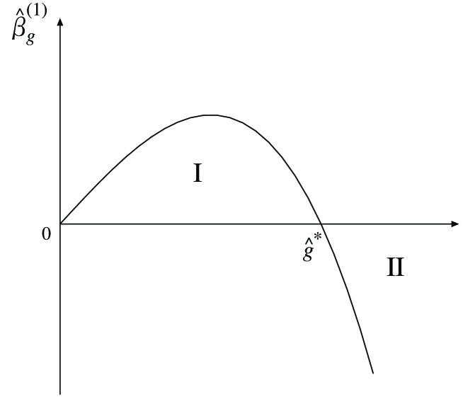
Figure 1: The generic form of $\hat{\beta}_{g}^{(1)}$.

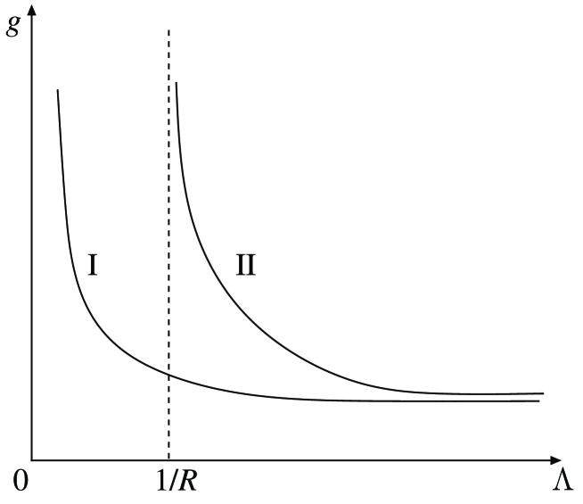
Figure 2: The evolution of the gauge coupling in two phases. Phase I is the decoupling phase, while phase II is the strongly interacting phase.

The generic form of the $\beta$ function $\hat{\beta}^{(1)}_{g}$ [see Eq. (6)] is shown in Fig. 1, in which two phases are indicated by I and II. The renormalization group (RG) flow of the gauge coupling $g$ in two phases are different, as shown in Fig. 2. As the energy scale $\Lambda$ decreases from a higher value, the flow of the phase II develops into a “Landau” pole near the compactification scale $\sim 1/R$, while the coupling in phase I has no such singularity near $\sim 1/R$. That is, the theory in phase II will become strongly interacting near $\sim 1/R$, and it will be unlikely that the massive Kaluza-Klein excitations (which seem to exist at the classical level) decouple . Only if the theory is in phase I there will be a chance for the massive Kaluza-Klein excitations to decouple and hence to have a renormalizable, low-energy effective theory below $\sim 1/R$. We regard this as a constraint on the gauge coupling. So the theory should be in phase I; in the decoupling phase.

3 Nontriviality of SUSY GUTs with extra dimensions

We assume that $\delta=D-4$ dimensions are compactified on an orbifold $S^{1}/Z_{2}$ of a fixed radius $R$. We denote the $D$-dimensional coordinates by $z_{M}~{}(M=1,\dots,D)$, while the four-dimensional ones by $x_{\mu}~{}(\mu=1,\dots,4)$ and the $\delta$-dimensional ones by $y_{a}~{}(a=1,\dots,\delta)$. A generic field $\phi(z)$, bosonic or fermionic, satisfying the periodic boundary condition

$$\phi(x,y) = \phi(x,y+2\pi R)~{}$$ (8)

with the parity property under $y_{a}\to-y_{a}$

$$\phi = \phi~{}|_{y_{a}\to-y_{a}}~{}~{}\mbox{for}~{}~{}a\in E_{+}~{}~{}\mbox{and}~{}~{}\phi=-\phi~{}|_{y_{a}\to-y_{a}}~{}~{}\mbox{for}~{}~{}a\in E_{-}$$ (9)

can be expanded as

$$\phi(x,y) = ~{}\sum_{{\bf n}=0}^{\infty}~{}~{}\sum_{{\bf m}=1}^{\infty}~{}\phi_{{\bf n},{\bf m}}(x)~{}\Pi_{a\in E_{+}}~{}\cos(n_{a}y_{a}/R)~{}\Pi_{b\in E_{-}}~{}\sin(m_{b}y_{b}/R)~{},$$ (10)

where we have divided $E=\{a=1,\dots,\delta\}$ into $E_{+}$ and $E_{-}$ corresponding to the parity property of $\phi$. The coefficients $\phi_{{\bf n},{\bf m}}(x)$ exhibit the Kaluza-Klein tower, and $\phi_{{\bf 0},{\bf 0}}(x)$ is the zero mode, which is absent if $\phi$ has an odd parity. The Kaluza-Klein modes other than the zero mode are massive $\sim O(1/R)$ in four dimensions. Since we consider GUTs, a certain set of the zero modes also become massive after a spontaneous symmetry breaking of the unifying gauge group $G$. Their masses are of the order of the spontaneous symmetry breaking or of the GUT scale $M_{G}$. The presence of the fields that exist only at a lower-dimensional boundary, the boundary fields, is allowed in the case of the orbifold compactification. Here we restrict ourselves only to the boundary fields that are located at our four-dimensional Minkowski space. They have no Kaluza-Klein massive partners, and they count among the zero modes.

Our main assumptions in considering SUSY GUTs are that (i) in the zero mode sector of the Kaluza-Klein tower, softly broken, four-dimensional $N=1$ supersymmetry is realized and (ii) the massive Kaluza-Klein modes form $N=2$ supermultiplets. The first assumption can be simply satisfied thanks to the orbifold compactification, and the second one can also be easily satisfied because a simple supersymmetry in higher dimensions always contains more than one supersymmetry in four dimensions. Correspondingly, the matter supermultiplets of the zero mode sector are $N=1$ chiral supermultiplets,

$$\Phi_{I} = (\phi_{I}~{},~{}\psi_{I})~{},$$ (11)

where $\phi_{I}~{}(\psi_{I})$ is the scalar (fermionic) component, and $I$ stands for color and flavor. The most general (cubic) form of the Yukawa term of the zero mode sector at the four-dimensional boundary takes the form

$$S_{0}^{Y} = \int d^{4}x~{}\frac{1}{2}~{}\sum_{I,J,K}Y^{IJK}~{}\psi_{I}\psi_{J}\phi_{K}~{}+\mbox{h.c.},$$ (12)

where the Yukawa couplings $Y^{IJK}$ are assumed to be completely symmetric in the indices. Although we have to add a set of certain terms to the above action $S_{0}^{Y}$ to make the boundary theory supersymmetric and gauge invariant, the complete space of the dimensionless couplings of the boundary theory, by virtue of $N=1$ supersymmetry, is spanned by the gauge coupling $g$ and the Yukawa couplings $Y^{IJK}$: That is, no additional dimensionless couplings are present.

If the contributions of the massive Kaluza-Klein modes to the RG functions ($\beta$ functions and anomalous dimensions $\gamma$) are suppressed, we have the well-known four-dimensional formulae [27]:

$$\beta^{(1)}_{g} = \frac{g^{3}}{16\pi^{2}}\,[\,\sum_{a}\,l(R_{a})-3\,C_{2}(G)\,]~{}$$ (13)

at one-loop, where $l(R_{a})$ is the Dynkin index of the representation $R_{a}$ and $C_{2}(G)$ is the quadratic Casimir of the adjoint representation of the gauge group $G$. The $\beta$ functions of $Y^{IJK}$ are related to the anomalous dimensions $\gamma_{I}^{(1)\,J}$ as [27]

$$\beta_{Y}^{(1)IJK} = \sum_{P}~{}Y^{IJP}\,\,\gamma_{P}^{(1)\,K}+(K\leftrightarrow I)+(K\leftrightarrow J)~{},$$ (14)

$$\gamma_{I}^{(1)\,J} = \frac{1}{16\pi^{2}}~{}[\,\frac{1}{2}\sum_{P,Q}~{}Y_{IPQ}Y^{JPQ}-2\delta^{J}_{I}\,g^{2}\,C_{2}(I)\,]~{},$$ (15)

where $C_{2}(I)$ is the quadratic Casimir of the representation $R_{I}$, and $Y^{IJK}=(Y_{IJK})^{*}$.

The Kaluza-Klein tower modifies the RG functions to the form that describes the power-law behavior of the couplings. The inclusion of the contribution of the massive Kaluza-Klein modes to the RG functions is straightforward, because they form $N=2$ supermultiplets by assumption and we may use the nonrenormalization theorem for $N=2$ supersymmetry [28]. Among the zero modes, there are those that have no massive partner modes, and they do not contribute to the power law behavior of the couplings. Therefore, their contributions to the RG functions in the $\Lambda\to\infty$ limit are much smaller compared with those coming from the infinite tower of the massive modes, i.e.,

$$\beta_{g}^{(1)} \simeq \frac{g^{3}}{16\pi^{2}}\,[\,\sum_{a^{\prime}}\,l(R_{a^{\prime}})-2\,C_{2}(G)\,]~{}X_{\delta}~{}(\Lambda R)^{\delta}~{},$$ (16)

$$\beta_{Y}^{(1)IJK} \simeq \frac{1}{16\pi^{2}}\,[~{}\frac{1}{2}~{}\sum_{P,L,M}{}^{\prime}~{}Y^{IJP}Y_{PLM}Y^{KLM}-2\sum_{P}{}^{\prime}~{}Y^{IJP}\,\delta_{P}^{K}~{}g^{2}\,C_{2}(K)$$ (17)

$$+(K\leftrightarrow I)+(K\leftrightarrow J)~{}]~{}X_{\delta}~{}(\Lambda R)^{\delta}~{},$$

where $X_{\delta}$ is given in Eq. (4). Here $\sum_{a^{\prime}}$ denotes the sum over $N=2$ hypermultiplets, and $\sum{}^{\prime}$ denotes the sum in which only the possibilities that contribute to the power law behavior are included. In deriving the $\beta$ functions (16) and (17), we have used the fact that the contributions of each excited Kaluza-Klein state to the anomalous dimension has the same form as a massless mode contribution [6].

Now according to the discussion in the previous section, we go over to the effective expansion parameters: As for the gauge coupling, it is defined in Eq. (5), and similarly we can find them for the Yukawa couplings. It is however more convenient to work with

$$\tilde{Y}^{IJK} = \frac{Y^{IJK}}{g}=\frac{Y^{IJK}(2\pi R\Lambda)^{\delta/2}}{g(2\pi R\Lambda)^{\delta/2}}=\frac{\hat{Y}^{IJK}}{\hat{g}}~{},$$ (18)

which yields the following system of the $\beta$ functions at large $\Lambda$:

$$\hat{\beta}_{g} = \Lambda\frac{d\hat{g}}{d\Lambda}=\frac{\delta}{2}\hat{g}-\frac{\hat{g}^{3}}{16\pi^{2}}\,[\,2\,C_{2}(G)\sum_{a^{\prime}}-\,l(R_{a^{\prime}})\,]~{}\frac{X_{\delta}}{(2\pi)^{\delta}}+\cdots~{},$$ (19)

$$\tilde{\beta}_{Y}^{IJK} = \Lambda\frac{d\tilde{Y}^{IJK}}{d\Lambda}=\hat{g}^{2}~{}[~{}-\tilde{Y}^{IJK}S(IJK)+(~{}\frac{1}{2}~{}\sum_{P,L,M}{}^{\prime}~{}\tilde{Y}^{IJP}\tilde{Y}_{PLM}\tilde{Y}^{KLM}~{})$$ (20)

$$+(K\leftrightarrow I)+(K\leftrightarrow J)~{}]~{}\frac{X_{\delta}}{(2\pi)^{\delta}}+\cdots~{},$$

where $\cdots$ stands for higher order contributions, and

$$\tilde{Y}^{IJK}S(IJK) = \tilde{Y}^{IJK}(\,\sum_{a^{\prime}}\,l(R_{a^{\prime}})-2\,C_{2}(G)\,)$$ (21)

$$+[~{}2\sum_{P}{}^{\prime}~{}\tilde{Y}^{IJP}\,\delta_{P}^{K}\,C_{2}(K)~{}]+[K\leftrightarrow I]+[K\leftrightarrow J]~{}.$$

Note that the sum in Eq. (21) (though it is proportional to $\tilde{Y}^{IJK}$) is not equal to $2\tilde{Y}^{IJK}(C_{2}(I)+C_{2}(J)+C_{2}(K))$, because the sum $\sum_{P}{}^{\prime}$ is taken over only the possibilities that contribute to the power law behavior.

From the $\beta$ functions (19) and (20) we see that

$$\tilde{Y}^{IJK} = 0$$ (22)

is an ultraviolet stable fixed point, if

$$S(IJK) > 0~{}~{}\mbox{for all}~{}~{}I,J,K~{}~{}\mbox{and}~{}~{}2\,C_{2}(G)-\sum_{a^{\prime}}\,l(R_{a^{\prime}})>0~{}$$ (23)

are satisfied. According to our assumption, the theory exists nonperturbatively if the conditions (23) are satisfied. If $S(IJK)>0$, on the other hand, there will be a certain set of infrared fixed points. That is, the stable manifold (the set of points in the space of $\tilde{Y}^{IJK}$ that can be initial points of a RG flow approaching the ultraviolet fixed point (22) ) must be a subspace of the space of $\tilde{Y}^{IJK}$. Therefore, the requirement of the nonperturbative existence implies that the Yukawa couplings at the GUT scale $M_{G}$ should be in the stable manifold. If all the Yukawa couplings are small compared with the unified gauge coupling, this condition can be easily satisfied. If however some of the Yukawa couplings, e.g. the top quark Yukawa coupling, are comparable with the unified gauge coupling in the magnitude, this condition can be a severe condition. The situation depends on the model considered of course. In the next section we consider a concrete gauge model based on the gauge group $SU(5)$ and discuss how the requirements coming from the nontriviality can be satisfied.

4 Application to the minimal SUSY $SU(5)$ GUT

4.1 The model and its nontriviality

The three generations of quarks and leptons are accommodated by six chiral $N=1$ superfields $\Psi^{i}({\bf 10})$ and $\Phi^{i}(\overline{\bf 5})$, where $i$ runs over the three generations. The superfield $\Sigma({\bf 24})$ is used to break $SU(5)$ down to $SU(3)_{\rm C}\times SU(2)_{\rm L}\times U(1)_{\rm Y}$, and $H({\bf 5})$ and $\overline{H}({\overline{\bf 5}})$ (which form an $N=2$ hypermultiplet) are two Higgs superfields appropriate for electroweak symmetry breaking. We assume that the matter superfields $\Psi^{i}({\bf 10})$ and $\Phi^{i}(\overline{\bf 5})$ are boundary fields so that they have no Kaluza-Klein excitations, and that the $4+\delta$-dimensional bulk theory is an $N=2$ supersymmetric Yang-Mills theory based on $G=SU(5)$ that contains a hypermultiplet in the fundamental representation of $G$. The cubic part of the boundary superpotential is given by

$$W = \sum_{i,j}^{3}\frac{G_{U}^{ij}}{4}\,\epsilon^{\alpha\beta\gamma\delta\tau}\,\Psi^{(i)}_{\alpha\beta}\Psi^{(j)}_{\gamma\delta}H_{\tau}+\sum_{i,j}^{3}\sqrt{2}\,G_{D}^{ij}\,\Phi^{(i)\alpha}\Psi^{(j)}_{\alpha\beta}\overline{H}^{\beta}+\frac{g_{\lambda}}{3}\,\Sigma_{\alpha}^{\beta}\Sigma_{\beta}^{\gamma}\Sigma_{\gamma}^{\alpha}~{},$$ (24)

where $\alpha,\beta,\ldots$ are the $SU(5)$ indices, and $G_{U}^{ij}$ and $G_{D}^{ij}$ are the Yukawa couplings. The $\overline{H}\Sigma H$ term is a part of the $N=2$ gauge interaction and belongs to the bulk action. To make the theory realistic, we have to have the correct pattern of spontaneous symmetry breaking of gauge symmetries, soft-supersymmetry-breaking (SSB) terms, and neutrino masses and their mixing. Note that only operators with dimensions less than four are responsible to satisfy these phenomenologically important requirements. Since however the contribution of these low-dimensional operators to the high energy behavior of the theory decreases with an increasing energy scale $\Lambda$, we ignore them in the following discussions.

Given the model, it is straightforward to compute the one-loop RG functions. We find that the one-loop anomalous dimensions of the chiral superfields are given by

$$16\pi^{2}~{}\gamma_{10} = [\,-\frac{36}{5}\,g^{2}+3\,G_{U}^{{\dagger}}G_{U}+2\,G_{D}^{{\dagger}}G_{D}\,]~{}X_{\delta}~{}(R\Lambda)^{\delta}~{},$$ (25)

$$16\pi^{2}~{}\gamma_{\bar{5}} = [\,-\frac{24}{5}\,g^{2}+4\,G_{D}^{{\dagger}}G_{D}\,]~{}X_{\delta}~{}(R\Lambda)^{\delta}~{},$$ (26)

$$16\pi^{2}~{}\gamma_{H} = 3\,\mbox{Tr}G_{U}G_{U}^{{\dagger}}~{},$$ (27)

$$~{}16\pi^{2}~{}\gamma_{\bar{H}} = 4\,\mbox{Tr}G_{D}G_{D}^{{\dagger}}~{},$$ (28)

$$16\pi^{2}~{}\gamma_{24} = [\,\frac{21}{5}\,g^{2}_{\sigma}-9\,g^{2}\,]~{}X_{\delta}~{}(R\Lambda)^{\delta}~{},$$ (29)

where $X_{\delta}$ is defined in Eq. (4). Using Eqs. (16) and (17) we then obtain the one-loop $\beta$ functions of the Yukawa couplings, where we use the fact that the anomalous dimensions of the Higgs supermultiplets vanish thanks to $N=2$ supersymmetry. Since we are interested in the $\Lambda\to\infty$ limit, only leading contributions in the limit,

$$16\pi^{2}~{}\beta_{g} \simeq -9g^{3}~{}X_{\delta}~{}(R\Lambda)^{\delta}~{},$$ (30)

$$~{}16\pi^{2}~{}\beta_{U} \simeq G_{U}~{}[\,-\frac{72}{5}\,g^{2}+6\,G_{U}^{{\dagger}}G_{U}+4\,G_{D}^{{\dagger}}G_{D}\,]~{}X_{\delta}~{}(R\Lambda)^{\delta}~{},$$ (31)

$$~{}16\pi^{2}~{}\beta_{D} \simeq G_{D}~{}[\,-12\,g^{2}+3\,G_{U}^{{\dagger}}G_{U}+6\,G_{D}^{{\dagger}}G_{D}\,]~{}X_{\delta}~{}(R\Lambda)^{\delta}~{},$$ (32)

$$16\pi^{2}~{}\beta_{\sigma} \simeq g_{\sigma}~{}[\,-27\,g^{2}+\frac{63}{5}\,g^{2}_{\sigma}\,]~{}X_{\delta}~{}(R\Lambda)^{\delta}~{},$$ (33)

should be considered. According to the discussion of the previous section, we now go over to the tide-couplings [defined in Eq. (18)], and find that the corresponding one-loop $\beta$ functions in the $\Lambda\to\infty$ limit can be written as

$$16\pi^{2}~{}\tilde{\beta}_{U}/\hat{g}^{2} = \tilde{G}_{U}~{}[\,-\frac{27}{5}\,+6\,\tilde{G}_{U}^{{\dagger}}\tilde{G}_{U}+4\,\tilde{G}_{D}^{{\dagger}}\tilde{G}_{D}\,]~{}\frac{X_{\delta}}{(2\pi)^{\delta}}~{},$$ (34)

$$16\pi^{2}~{}\tilde{\beta}_{D}/\hat{g}^{2} = \tilde{G}_{D}~{}[\,-3\,+3\,\tilde{G}_{U}^{{\dagger}}\tilde{G}_{U}+6\,\tilde{G}_{D}^{{\dagger}}\tilde{G}_{D}\,]~{}\frac{X_{\delta}}{(2\pi)^{\delta}}~{},$$ (35)

$$16\pi^{2}~{}\tilde{\beta}_{\sigma}/\hat{g}^{2} = \tilde{g}_{\sigma}~{}[\,-18+\frac{63}{5}\,\tilde{g}^{2}_{\sigma}\,]~{}\frac{X_{\delta}}{(2\pi)^{\delta}}~{},$$ (36)

where $\hat{g}$ is defined in Eq. (5). Moreover, the phenomenological requirements from the mass of leptons and quarks as well as from the proton decay [29, 30] imply that the Yukawa couplings for the top and bottom quarks, $G_{U}^{33}=G_{t}$ and $G_{D}^{33}=G_{b}$, are the largest couplings compared with the other Yukawa couplings, and therefore, to investigate approximately the high energy behavior of the theory, it is sufficient to consider the following set of the $\beta$ functions:

$$16\pi^{2}~{}\frac{\tilde{\beta}_{t}}{\hat{g}^{2}} = \tilde{G}_{t}~{}[\,-\frac{27}{5}\,+6\,\tilde{G}_{t}^{2}+4\,\tilde{G}_{b}^{2}\,]~{}\frac{X_{\delta}}{(2\pi)^{\delta}}~{},$$ (37)

$$16\pi^{2}~{}\frac{\tilde{\beta}_{b}}{\hat{g}^{2}} = \tilde{G}_{b}~{}[\,-3\,+3\,\tilde{G}_{t}^{2}+6\,\tilde{G}_{b}^{2}\,]~{}\frac{X_{\delta}}{(2\pi)^{\delta}}~{}.$$ (38)

We thus have arrived at a simple system defined by Eqs. (37) and (38) that has four fixed points

$$(~{}\tilde{G}_{t}^{*2},\tilde{G}_{b}^{*2}~{}) = (~{}0,0~{})~{},~{}(~{}\frac{17}{20},\frac{3}{40}~{})~{},(~{}\frac{9}{10},0~{})~{},(~{}0,\frac{1}{2}~{})~{}$$ (39)

in the two-dimensional space of couplings $\tilde{G}_{t}^{2}$ and $\tilde{G}_{b}^{2}$, which are shown in Fig. 3. As we have seen in the previous section, the origin $(~{}0,0~{})$ is an ultraviolet-stable fixed point. The point $(~{}17/20,3/40~{})$ is an infrared stable fixed point (the Pendleton-Ross fixed point [31]), while for the other two points there exist attractive as well as repulsive directions. We find that the direction perpendicular to the $\tilde{G}_{b}^{2}$ axis is the infrared-attractive direction for the fixed point $(~{}9/10,0~{})$, and similarly, the direction perpendicular to the $\tilde{G}_{t}^{2}$ axis is the one for $(~{}0,1/2)$. In Fig. 3 we show some representative RG flows, and as we can see from the figure, the stable manifold is a finite region in the space of $\tilde{G}_{t}^{2}$ and $\tilde{G}_{b}^{2}$. The critical lines that go from the infrared stable point $(~{}17/20,3/40~{})$ toward the end points $(~{}9/10,0~{})$ and $(~{}0,1/2~{})$ define the boundary of the stable manifold. We emphasize that the result above is independent of the number of the extra dimensions $\delta$ and the scale $\Lambda$.

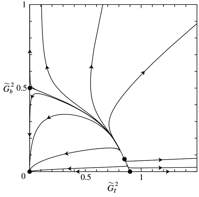
Figure 3: RG flows in the space of $\tilde{G}_{t}^{2}$ and $\tilde{G}_{b}^{2}$. The fixed points are denoted by a bullet.

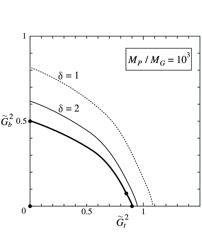
Figure 4: The stable manifold (bounded by the bold line) in the space of $\tilde{G}_{t}^{2}$ and $\tilde{G}_{b}^{2}$. The regions extended by the relaxed nontriviality requirement are also shown; the dotted, straight boundary lines correspond to $\delta=1,2$, respectively. As for $\delta=0$, the whole region in Fig. 4 satisfies the relaxed nontriviality requirement.

The nontriviality requirement above could be to strong; it is a requirement in the $\Lambda\to\infty$ limit. It can be relaxed so as to require for the couplings not to develop into a Landau pole before the Planck scale $M_{P}$. Since the above result on the fixed points (39) is independent on the energy scale $\Lambda$, especially on the actual value of the unification scale $M_{G}$, the ratio $M_{P}/M_{G}$ can take any value greater than $\sim 10^{3}$. Clearly, the smaller the ratio is, the milder is the relaxed nontriviality requirement. In Fig. 4 we show how the allowed region is extended by relaxing of the nontriviality requirement in the case of $M_{P}/M_{G}=10^{3}$. The relaxed condition depends on the number of the extra dimensions $\delta$. We have considered three cases $\delta=0,1$ and $2$ in Fig. 4, where the stable manifold is bounded by the bold line. As we can see from Fig. 4, the extensions for $\delta=1$ and $2$ are very small. This is a consequence of the power law running of the couplings; the couplings evolve faster in extra dimensions as the energy scale varies, and so the Landau pole can be faster reached compared with the case of the logarithmic running. Therefore, the initial point cannot be very far from the stable manifold. As for the logarithmic running ($\delta=0$) , we found that the whole region of Fig. 4 satisfies the relaxed nontriviality requirement ($M_{P}/M_{G}=10^{3}$), justifying our statement above. In the next subsection we would like to investigate phenomenological consequences from the nontriviality requirement.

4.2 The model between $1/R$ and $M_{G}$

To be more specific we assume that the extra dimensions are large, i.e. $1/R<1/10^{16}$ GeV, and that for energies below $1/R$ the MSSM is the effective theory. For the energy scale between $1/R$ and $M_{G}$, the effective theory is exactly the one proposed in Ref. [6], in which only the gauge boson and Higgs supermultiplets of the MSSM have a tower of Kaluza-Klein states and the lepton and quark supermultiplets have no tower of Kaluza-Klein states. Correspondingly, the one-loop $\beta$-functions for the energy scales between $1/R$ and $M_{G}$ become [6]

$$16\pi^{2}\beta_{1} = g_{1}^{3}~{}[6+\frac{6}{5}(X_{\delta}/2)(\Lambda R)^{\delta}]~{},$$ (40)

$$16\pi^{2}\beta_{2} = g_{2}^{3}~{}[4-6(X_{\delta}/2)(\Lambda R)^{\delta}]~{},$$ (41)

$$16\pi^{2}\beta_{3} = g_{3}^{3}~{}[3-12(X_{\delta}/2)(\Lambda R)^{\delta}]~{},$$ (42)

$$16\pi^{2}\beta_{t} = G_{t}~{}[3G_{t}^{2}-\frac{3}{10}g_{1}^{2}-\frac{3}{2}g_{2}^{2}$$ (44)

$$+(X_{\delta}/2)~{}(\Lambda R)^{\delta}(6G_{t}^{2}+2G_{b}^{2}-\frac{17}{15}g_{1}^{2}-3g_{2}^{2}-\frac{32}{3}g_{3}^{2})]~{},$$

$$16\pi^{2}\beta_{b} = G_{b}~{}[3G_{b}^{2}+G_{\tau}^{2}-\frac{3}{10}g_{1}^{2}-\frac{3}{2}g_{2}^{2}$$ (46)

$$+(X_{\delta}/2)~{}(\Lambda R)^{\delta}(2G_{t}^{2}+6G_{b}^{2}-\frac{1}{3}g_{1}^{2}-3g_{2}^{2}-\frac{32}{3}g_{3}^{2})]~{},$$

$$16\pi^{2}\beta_{\tau} = G_{\tau}~{}[3G_{b}^{2}+G_{\tau}^{2}-\frac{3}{10}g_{1}^{2}-\frac{3}{2}g_{2}^{2}$$ (48)

$$+(X_{\delta}/2)~{}(\Lambda R)^{\delta}(6G_{\tau}^{2}-3g_{1}^{2}-3g_{2}^{2})]~{},$$

where $g_{1,2,3}$ are the gauge couplings, $G_{t,b,\tau}$ are the Yukawa couplings for the top, bottom and tau, in the MSSM, respectively. We have neglected other Yukawa couplings, and use has been made of the fact that the anomalous dimensions of the Higgs supermultiplets due to $N=2$ supersymmetry in the excited sector vanish between $1/R$ and $M_{G}$ [28].

4.3 The lower bound of $\tan\beta$

In what follows we will consider only the case with $\delta=1$. Moreover, to simplify the situation, we assume that there exists a uniform SUSY threshold $M_{SUSY}$. We study the evolution of the couplings below $1/R$ at the two-loop level , along with the experimental inputs [33]; the tau mass $M_{\tau}=1.777~{}{\rm GeV}$, the $Z$ gauge boson mass $M_{Z}=91.187~{}{\rm GeV}$, the effective electromagnetic coupling $\alpha^{-1}_{\rm EM}(M_{Z})=127.9$ at $M_{Z}$, and the Weinberg mixing angle $\sin^{2}\theta_{W}(M_{Z})=0.2312$ in the modified minimal subtraction scheme. The experimental value of the physical top mass is given by [33]

$$M_{t} = (174.3\pm 5.1)~{}~{}\mbox{GeV}~{}.$$ (49)

At the SUSY threshold $M_{SUSY}$ we require that the matching conditions,

$$G_{t}^{\rm SM} = G_{t}\,\sin\beta~{},~{}G_{b}^{\rm SM}~{}=~{}G_{b}\,\cos\beta~{},~{}G_{\tau}^{\rm SM}~{}=~{}G_{\tau}\,\cos\beta~{},$$

$$\lambda = \frac{1}{4}(\frac{3}{5}g^{2}_{1}+g^{2}_{2})\,\cos^{2}2\beta~{},$$ (50)

should be satisfied, where $G_{i}^{\rm SM}~{}(i=t,b,\tau)$ are the SM Yukawa couplings and $\lambda$ is the Higgs self-coupling. This is our definition of $\tan\beta$. (There are MSSM threshold corrections to this matching condition [34, 35], which we ignore in the following discussion.) For a given set of the initial values of $G_{t}$ and $G_{b}$ at $M_{G}$, the top quark mass $M_{t}$ is no longer a free parameter and can be computed, where we use the formula [36, 34]

$$M_{t} = m_{t}(M_{t})\,[\,1+\frac{4}{3}\frac{\alpha_{3}(M_{t})}{\pi}+10.95\,(\frac{\alpha_{3}(M_{t})}{\pi})^{2}-0.3\frac{\alpha_{t}(M_{t})}{\pi}\,]~{}.$$ (51)

Here $\alpha_{3}=g_{3}^{2}/4\pi$, $\alpha_{t}=(G_{t}^{SM})^{2}/4\pi$, and $m_{t}(\mu)$ is the running top mass in the modified minimal subtraction scheme and given by

$$m_{t}(\mu) = \frac{1}{\sqrt{2}}G_{t}^{MS}(\mu)\,v(\mu)~{}\mbox{with}~{}~{}v(M_{Z})=246.22~{}\mbox{GeV}~{},$$ (52)

where $v$ is the vacuum expectation value of the SM Higgs field which is made of the two Higgs fields of the MSSM. The mass of the bottom quark can suffer from a large correction from the SSB terms [34, 35]. But we do not take into account them in the present analysis, because we do not consider the SSB terms.

Given all the facilities for the RG evolution of the couplings, we choose a value for $\tan\beta$ with the top mass varying from $170$ to $180$ GeV and let evolve the couplings from $M_{Z}$ to $M_{G}$ (at which the gauge coupling unification and the $b-\tau$ unification is realized). We then calculate the ratio

$$k_{t} = \frac{G_{t}^{2}}{g_{G}^{2}}=\tilde{G}_{t}^{2}$$ (53)

at $M_{G}$ as a function of $\tan\beta$, where $g_{G}$ is the unified gauge coupling. The results are shown in Figs. 5, 6 and 7. In Fig. 5 we vary $\tan\beta$ from $1$ to $60$ with $M_{SUSY}=1$ TeV, where the straight (dotted) line stands for $1/R=10^{14}(10^{5})$ GeV. The range of smaller $\tan\beta$ are plotted in Fig. 6 and 7; Fig. 6 shows the $M_{SUSY}$ dependence for $1/R$ fixed at $10^{14}$ GeV, while Fig. 7 shows the $R$ dependence for $M_{SUSY}$ fixed at $1$ GeV. We see from these figures that the value of $k_{t}$ increases rapidly as $\tan\beta$ approaches $\sim 2$ from larger values, and that this feature does not depend very much on $R$ and $M_{SUSY}$. Comparing this result with Fig. 4 (which shows the region in the $\tilde{G}_{t}^{2}$-$\tilde{G}_{b}^{2}$ plane satisfying the nontriviality requirement), we see that for a small value ($\mathrel{\mathchoice{\vbox{\offinterlineskip\halign{$\m@th\displaystyle\hfil#\hfil$\cr<\crcr\sim\crcr} }}{\vbox{\offinterlineskip\halign{$\m@th\textstyle\hfil#\hfil$\cr<\crcr\sim\crcr} }}{\vbox{\offinterlineskip\halign{$\m@th\scriptstyle\hfil#\hfil$\cr<\crcr\sim\crcr} }}{\vbox{\offinterlineskip\halign{$\m@th\scriptscriptstyle\hfil#\hfil$\cr<\crcr\sim\crcr} }}}2$) of $\tan\beta$, leading to a large value of $k_{t}$, the theory cannot be made nontrivial.

As we have seen in Sect.4.2, the difference between the power law and logarithmic running is how fast the RG evolution develops into a Landau pole as $\Lambda$ increases. Moreover, the more there exist extra dimensions, the faster is the evolution, and hence the closer to the stable manifold is the region satisfying the relaxed nontriviality requirement (see in Fig. 4). From this observation we conclude that the presence of the extra dimensions prefers a large value ($\mathrel{\mathchoice{\vbox{\offinterlineskip\halign{$\m@th\displaystyle\hfil#\hfil$\cr>\crcr\sim\crcr} }}{\vbox{\offinterlineskip\halign{$\m@th\textstyle\hfil#\hfil$\cr>\crcr\sim\crcr} }}{\vbox{\offinterlineskip\halign{$\m@th\scriptstyle\hfil#\hfil$\cr>\crcr\sim\crcr} }}{\vbox{\offinterlineskip\halign{$\m@th\scriptscriptstyle\hfil#\hfil$\cr>\crcr\sim\crcr} }}}2$) of $\tan\beta$. As it is known [37], the mass of the MSSM Higgs depends on $\tan\beta$. The search for the Higgs particle at LEP2 have already excluded the range of $tan\beta$ [33, 38]

$$\left\{\begin{array}[]{l}0.5\sim 2.3\\ 0.7\sim 1.9\end{array}\right.~{}~{}\mbox{for}~{}~{}M_{t}=\left\{\begin{array}[]{l}175\\ 180\end{array}\right.~{}\mbox{GeV}~{}.$$ (58)

So today’s possible observation of the Higgs particle [14] might be an indication of the existence of extra dimensions.

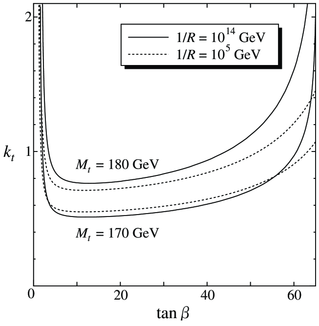
Figure 5: $k_{t}$ as a function of $\tan\beta$ for $1/R=10^{14}$ (straight) and $10^{5}$ (dotted) GeV with $M_{SUSY}=1$ TeV.

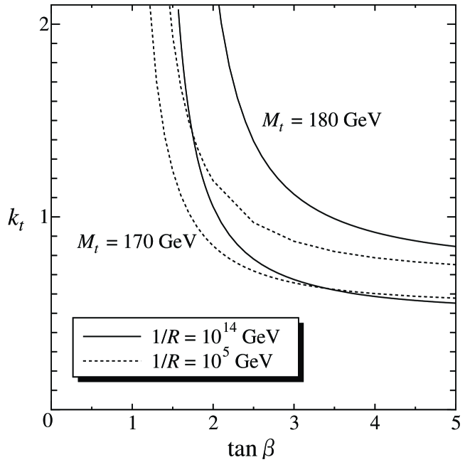
Figure 6: The same as Fig. 5 near $\tan\beta=2$.

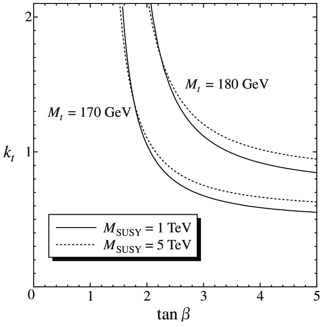
Figure 7: The $M_{SUSY}$ dependence of $k_{t}$ near $\tan\beta=2$ with $1/R=10^{14}$ GeV.

5 Conclusion

Our starting point was to assume that the result obtained from the Monte Carlo simulations on the nonperturbative existence of the Yang-Mills theory in five dimensions [11] can be applied to a more general class of higher-dimensional unified gauge theories. The first nontrivial requirement is that the theory should be in phase I of Fig. 1, because otherwise the massive Kaluza-Klein excitations would not decouple at low energies. Then we have derived the conditions (23) imposed by the nontriviality requirement on the supersymmetric gauge theories containing matter superfields, where we have also considered relaxing the nontriviality requirement. These results have been applied to a concrete SUSY GUT based on $SU(5)$, and we have found, comparing Fig. 4 with Figs. 5, 6 and 7 that the model prefers a large value ($\mathrel{\mathchoice{\vbox{\offinterlineskip\halign{$\m@th\displaystyle\hfil#\hfil$\cr>\crcr\sim\crcr} }}{\vbox{\offinterlineskip\halign{$\m@th\textstyle\hfil#\hfil$\cr>\crcr\sim\crcr} }}{\vbox{\offinterlineskip\halign{$\m@th\scriptstyle\hfil#\hfil$\cr>\crcr\sim\crcr} }}{\vbox{\offinterlineskip\halign{$\m@th\scriptscriptstyle\hfil#\hfil$\cr>\crcr\sim\crcr} }}}2$) of $\tan\beta$. Moreover it has been argued that this is not a model-specific feature, but a general feature of SUSY GUTs with extra dimensions.

Acknowledgments
This work is supported partially by the Ministry of Education, Science and Culture and by the Japan Society for the Promotion of Science. We would like to thank H. Nakano, D. Suematsu and H. Terao for useful discussions.

References

- [1] I. Antoniadis, Phys. Lett. B 246, 377 (1990); I. Antoniadis, C. Muñoz and M. Quirós, Nucl. Phys. B397, 515 (1993).
- [2] E. Witten, Nucl. Phys. B471, 135 (1996); P. Horava and E. Witten, Nucl. Phys. B460, 506 (1996); B475, 94 (1996).
- [3] J.D. Lykken, Phys. Rev. D 54, 3693 (1996).
- [4] N. Arkani-Hamed, S. Dimopoulos and G. Dvali, Phys. Lett. B 429, 263 (1998); Phys. Rev. D 59, 086004 (1999).
- [5] I. Antoniadis, N. Arkani-Hamed, S. Dimopoulos and G. Dvali, Phys. Lett. B 436, 257 (1998).
- [6] K. Dienes, E. Dudas and T. Gherghetta, Phys. Lett. B 436, 311 (1998); Nucl. Phys. B537, 47 (1999).
- [7] L. Randall and R. Sundrum, Phys. Rev. Lett. 83, 3370 (1999); ibid. 83, 4690 (1999); L. Lykken and L. Randall, J. High Energy Phys. 06, 014 (20000).
- [8] I. Antoniadis and K. Benakli, hep-ph/0007226.
- [9] M. Dine, Plenary Talk given at ICEP 2000, Osaka, Japan, July 27-August 2, 2000, hep-th/0010035.
- [10] K. Dienes, hep-ph/0004129; L. Hall, Plenary Talk at ICEP 2000, Osaka, Japan, July 27-August 2, 2000.
- [11] S. Ejiri, J. Kubo and M. Murata, Phys. Rev. D 62, 105025 (2000) .
- [12] M. Peskin, Phys. Lett. 94B, 161 (1980).
- [13] N. Cabibbo, L. Maiani, G. Parisi and R. Petronzio, Nucl. Phys. B158, 295 (1979); R. Dashen and H. Neuberger, Phys. Rev. Lett. 50, 1897 (1983); M. Lindner, Z. Phys. C31, 295 (1986); C. Kolda and H. Murayama, J. High Energy Phys. 0007, 35 (2000), references therein.
- [14] P. McNamara, Talk given at LEPC Seminar, November 3, 2000.
- [15] G. Burgers, F. Karsch, A. Nakamura and I.O. Stamatescu, Nucl. Phys. B304, 587 (1988).
- [16] T.R. Klassen, Nucl. Phys. B533, 557 (1998).
- [17] J. Engels, F. Karsch and T. Scheideler, Nucl. Phys. B564, 303 (2000).
- [18] S. Ejiri, Y. Iwasaki, and K. Kanaya, Phys. Rev. D 58, 094505 (1998).
- [19] M. Creutz, Phys. Rev. Lett. 43, 553 (1979).
- [20] H. Kawai, M. Nio and Y. Okamoto, Prog. Theor. Phys. 88, 341 (1992).
- [21] J. Nishimura, Mod. Phys. Lett. A 11, 3049 (1996).
- [22] T.R. Taylor and G. Veneziano, Phys. Lett. B 212, 47 (1988).
- [23] T. Kobayashi, J. Kubo, M. Mondragon and G. Zoupanos, Nucl. Phys. B550, 99 (1999); J. Kubo, H. Terao and G. Zoupanos, Nucl. Phys. B574, 495 (2000).
- [24] Z. Kakushadze and T. R. Taylor, Nucl. Phys. B562, 78 (1999).
- [25] N. Arkani-Hamed, H. Cheng, B.A. Dobresu and L.J. Hall, Phys. Rev. D 62, 096006 (2000).
- [26] M. Hashimoto, M. Tanabashi and K. Yamawaki, hep-ph/0010260.
- [27] I. Jack and D.R.T. Jones, Phys. Lett. B 333, 372 (1994); S.P. Martin and M.T. Vaughn, Phys. Rev. D 50, 2282 (1994); Y. Yamada, Phys. Rev. D 50, 3537 (1994), and references therein.
- [28] P. Howe, K. Stelle and P. West, Phys. Lett. B 124, 55 (1983); P. Howe, K. Stelle and P.K. Townsend, Nucl. Phys. B236, 125 (1984).
- [29] J. Hisano, H. Murayama and T. Yanagida, Nucl. Phys. B402, 46 (1993).
- [30] J. Kubo, M. Mondragón, M. Olechowski and G. Zoupanos, Nucl. Phys. B479, 25 (1996).
- [31] B. Pendleton and G.G Ross, Phys. Lett. B 98, 291 (1981); M. Lanzagorta and G.G. Ross, Phys. Lett. B 349, 319 (1995).
- [32] W. Zimmermann, Com. Math. Phys. 97, 211 (1985); R. Oehme and W. Zimmermann, Com. Math. Phys. 97, 569 (1985); J. Kubo, K. Sibold and W. Zimmermann, Nucl. Phys. B259, 331 (1985).
- [33] Particle Data Group, Eur. Phys. J. C15, 1 (2000).
- [34] L. Hall, R. Rattazzi and U. Sarid, Phys. Rev. D 50, 7048 (1994); M. Carena, M. Olechowski, S. Pokorski and C.E.M. Wagner, Nucl. Phys. B426, 269 (1994).
- [35] B.D. Wright, hep-ph/9404217.
- [36] H. Arason et al., Phys. Rev. D 46, 3945 (1992); V. Barger, M.S. Berger and P. Ohmann, Phys. Rev. D 47, 1093 (1993), and references therein.
- [37] Y. Okada, M. Yamaguchi and T. Yanagida, Prog. Theor. Phys. 85 1 (1991); H.E. Haber and R. Hempfling, Phys. Rev. Lett. 66, 1815 (1991); J. Ellis, G. Ridolfi and F. Zwirner, Phys. Lett. B 257, 83 (1991); R. Barbieri an M. Frigeni, Phys. Lett. B 258, 395 (1991); M. Carena, H.E. Haber, S. Heinemeyer, W. Hollik, C.E.M. Wagner and G. Weiglein, hep-ph/0001002, and references therein.
- [38] P. Igo-Kemenes, Plenary Talk given at ICEP 2000, Osaka, Japan, July 27-August 2, 2000.