FZJ-IKP(TH)-2000-26

Chiral dynamics in the presence of bound states:
kaon–nucleon interactions revisited

Abstract

We study the S–wave kaon–nucleon interactions for strangeness $S=-1$ in a novel relativistic chiral unitary approach based on coupled channels. Dispersion relations are used to perform the necessary resummation of the lowest order relativistic chiral Lagrangian. A good description of the data in the $K^{-}p$, $\pi\Sigma$ and $\pi\Lambda$ channels is obtained. We show how this method can be systematically extended to higher orders, emphasizing its applicability to any scenario of strong self–interactions where the perturbative series diverges even at low energies. Discussions about the differences to existing approaches employing pseudo–potentials in a regulated Lippmann–Schwinger equation are included. Finally, we describe the resonance content of our meson–baryon amplitudes and discuss its nature.

1. The $\bar{K}N$ ($K^{-}p,\bar{K}^{0}n$) interaction is of interest for nuclear, particle and astrophysics. It is characterized by large rescattering effects between different channels and by the presence of the $\Lambda(1405)$ resonance just below the $\bar{K}N$ threshold. From the theoretical point of view one expects that chiral symmetry severely constrains the interactions between the different channels. However, because of such large rescattering effects, for short unitarity corrections, pure meson–baryon chiral perturbation theory (CHPT) [1, 2, 3, 4, 5, 6] cannot be applied. In particular, the resonance $\Lambda(1405)$ can be never reproduced in such a perturbative framework at any finite order because it is not perturbative in the chiral counting. As a consequence of that, a proper way of resummation of these strong unitarity corrections in the chiral expansion is necessary. A similar situation can be found in the nucleon–nucleon system where the presence of shallow nuclear bound states invalidates the application of perturbative effective field theory techniques. The solution advocated in ref.[7] is to apply the chiral expansion to generate an “effective potential” which is then iterated in a Lippmann-Schwinger equation to calculate the whole S–matrix. Such ideas have been successfully pursued for $\bar{K}N$ scattering based on chiral Lagrangians and coupled channel pseudo–potentials in regulated Lippmann–Schwinger equations, see [10, 11]. In these studies the nonperturbative nature of the strangeness $S=-1$ S–wave kaon–nucleon interaction was clearly established. However, from the theoretical point of view, the methods employed in [10, 11] should further be improved. First, although chiral perturbation theory Lagrangians are used, a direct matching to the proper CHPT amplitudes is not done, an ingredient already stressed a decade ago in a different context [12]. Second, the results presented in [10, 11] show a strong sensitivity to the cut–off or regulator masses. This can be avoided e.g. by employing subtracted dispersion relations, with the added advantage that the subtraction constants can even be taken at some unphysical points, where they can be constrained by chiral symmetry (a nice example for this is the study of higher order corrections in eta decays in [13, 14]). Note that the usefulness of considering a subtraction scheme rather than a cut–off has also been stressed in [15]. By construction, our approach is fully relativistic and thus one never has to make recourse to any expansion in the inverse of the baryon mass, although that can be done if desired. Third, the explicit inclusion of resonance fields in these schemes is not at all obvious. This becomes of importance if one wants to decide whether a resonance is simply generated by the strong meson–baryon dynamics or also has a “preexisting” (quark model) component. Such questions have e.g. been addressed in the context of potential models of varying sophistication, see [16, 17]. We present here a general and alternative scheme to that of introducing a potential [7] in order to still apply chiral Lagrangians to those situations where the perturbative chiral expansion fails because of the strong self–interactions between the relevant degrees of freedom. Note that these strong interactions can even generate poles (e.g. bound states) in the S-matrix as it happens e.g. in some channels of the $\bar{K}N$, nucleon–nucleon and even of the meson–meson systems. The approach is based on coupled channel subtracted dispersion relations and on matching the general expression for the pertinent partial wave amplitudes to the results of any given CHPT calculation in a well defined chiral power counting. The method is suited to include the contributions of explicit resonance fields, if desired. It is a natural extension and reformulation of our previous work on pion–nucleon scattering [18]. Although our approach is more general, in this letter we only show that even starting from the lowest order tree–level amplitudes of the kaon–nucleon system, one can fairly well describe the threshold branching ratios and scattering data as well as the event distributions (note that we have developed an improved method for calculating these event distributions as shown below). We also give a detailed comparison to the existing approaches to underline the remarks made in this introduction.

2. The lowest order ${\cal O}(p)$ SU(3) meson–baryon Lagrangian compatible with chiral symmetry and its breakings, both spontaneous and explicit, and with parity and charge conjugation can be written as:

$${\mathcal{L}}=\langle i\bar{B}\gamma^{\mu}\partial_{\mu}B-m_{0}\bar{B}B+\frac{1}{2}D\,\bar{B}\gamma^{\mu}\gamma_{5}\left\{u_{\mu},B\right\}+\frac{1}{2}F\,\bar{B}\gamma^{\mu}\gamma_{5}[u_{\mu},B]\rangle$$ (1)

where $m_{0}$ stands for the (average) octet baryon mass in the chiral limit. The trace $\langle\ldots\rangle$ runs over the flavor indices and the axial-vector couplings $F$ and $D$ are subject to the constraint $F+D=g_{A}=1.26$. We use the values $D=0.8$ and $F=0.46$ extracted from hyperon decays [19]. Furthermore, we have $u_{\mu}=iu^{\dagger}(\partial_{\mu}U)u^{\dagger}=u_{\mu}^{\dagger}$, $U(\Phi)=u(\Phi)^{2}=\exp(i\sqrt{2}\Phi/F_{0})$, with $F_{0}$ the pseudoscalar decay constant in the chiral limit. The $3\times 3$ flavor–matrices $\Phi$ and $B$ are given by:

$$\Phi=\sum_{i}\frac{\lambda_{i}}{\sqrt{2}}\phi_{i} = \left(\begin{array}[]{ccc}\frac{1}{\sqrt{2}}\pi^{0}+\frac{1}{\sqrt{6}}\eta&\pi^{+}&K^{+}\\ \pi^{-}&-\frac{1}{\sqrt{2}}\pi^{0}+\frac{1}{\sqrt{6}}\eta&K^{0}\\ K^{-}&\bar{K}^{0}&-\frac{2}{\sqrt{6}}\eta\end{array}\right)~{},$$ (5)

$$B=\sum_{i}\frac{\lambda_{i}}{\sqrt{2}}B_{i} = \left(\begin{array}[]{ccc}\frac{1}{\sqrt{2}}\Sigma^{0}+\frac{1}{\sqrt{6}}\Lambda&\Sigma^{+}&p\\ \Sigma^{-}&-\frac{1}{\sqrt{2}}\Sigma^{0}+\frac{1}{\sqrt{6}}\Lambda&n\\ \Xi^{-}&\Xi^{0}&-\frac{2}{\sqrt{6}}\Lambda\end{array}\right)~{},$$ (9)

where the $\lambda_{i}$ are the usual SU(3) Gell-Mann matrices. Notice that for our purpose, it is not necessary to consider in eq.(1) external fields related i.e. to the electroweak interactions. From eq.(1) it is straightforward to write down the lowest order CHPT (i.e. tree level) $\phi_{i}B_{a}\rightarrow\phi_{j}B_{b}$ amplitude, denoted $T(ij,ab)$. It is given by the sum of the diagrams in fig.1:

$$T(ij,ab) = T_{s}(ij,ab)+T_{d}(ij,ab)+T_{c}(ij,ab)~{},$$ (10)

$$T_{s}(ij,ab) = \sum_{k=1}^{8}f_{abk}f_{ijk}\frac{NN^{\prime}}{F_{0}^{2}}\chi_{b}\left[W-m_{0}+\left(\vec{p}\cdot\vec{p}\,^{\prime}+i(\vec{p}\,^{\prime}\times\vec{p})\cdot\vec{\sigma}\right)\frac{W+m_{0}}{(NN^{\prime})^{2}}\right]\chi_{a}~{},$$

$$T_{d}(ij,ab) = -\sum_{k=1}^{8}(Dd_{jkb}+iFf_{jkb})(Dd_{ika}-iFf_{ika})\frac{NN^{\prime}}{F_{0}^{2}}\chi_{b}\left[-2m_{0}+\frac{s+3m_{0}^{2}}{W+m_{0}}\right.$$

$$+ \left.\frac{\vec{p}\cdot\vec{p}\,^{\prime}+i(\vec{p}\,^{\prime}\times\vec{p})\cdot\vec{\sigma}}{(NN^{\prime})^{2}}\left(2m_{0}+\frac{s+3m_{0}^{2}}{W-m_{0}}\right)\right]\chi_{a}~{},$$

$$T_{c}(ij,ab) = -\sum_{k=1}^{8}(Dd_{ikb}+iFf_{ikb})(Dd_{jka}-iFf_{jka})\frac{NN^{\prime}}{F_{0}^{2}}\chi_{b}\left[-2m_{0}-\frac{(W-m_{0})(u+3m_{0}^{2})}{u-m_{0}^{2}}\right.$$

$$+ \left.\frac{\vec{p}\cdot\vec{p}\,^{\prime}+i(\vec{p}\,^{\prime}\times\vec{p})\cdot\ \vec{\sigma}}{(NN^{\prime})^{2}}\left(2m_{0}-\frac{W+m_{0}}{u-m_{0}^{2}}(u+3m_{0}^{2})\right)\right]\chi_{a}~{},$$

Figure 1: Leading order tree level diagrams. Baryons and meson are depicted by solid and dashed lines, respectively. Shown are the seagull (s), direct (d) and crossed (c) graphs, in order.

where $f_{klm}$ and $d_{klm}$ are constants defined in terms of the commutators and anticommutators of the SU(3) Gell-Mann matrices in the usual way: $[\lambda_{k},\lambda_{l}]=2i\sum_{m=1}^{8}f_{klm}\lambda_{m}$, $\{\lambda_{k},\lambda_{l}\}=2\sum_{m=1}^{8}d_{klm}\lambda_{m}$, $W\equiv\sqrt{s}$ is the total centre–of–mass (c.m.) energy, and $u=(p-q^{\prime})^{2}$, with $p$ and $q^{\prime}$ the four–momentum of the initial baryon and final meson, respectively. In addition, $N=\sqrt{E_{0}+m_{0}}$ and $N^{\prime}=\sqrt{E^{\prime}_{0}+m_{0}}$, with $E_{0}$ and $E^{\prime}_{0}$ the c.m. energies of the initial and final baryons with masses $m_{0}$, in order. Finally, $\vec{p}$ and $\vec{p}\,^{\prime}$ are the c.m. three-momentum vectors of the baryons in the initial and final state, respectively and $\chi_{c}$, with $c=a$ or $b$, is a two component Pauli spinor. To calculate the previous expressions, we have considered one particle states $|\vec{p},\sigma\rangle$ with c.m. three–momentum $\vec{p}$ and spin component $\sigma$ normalized such that $\langle\vec{p},\sigma|\vec{p}\,^{\prime},\sigma^{\prime}\rangle=2p^{0}(2\pi)^{3}\delta^{(3)}(\vec{p}-\vec{p}\,^{\prime})\delta_{\sigma\sigma^{\prime}}$. Here, $p^{0}$ is the energy of the particle, $\delta^{(3)}(\vec{p}-\vec{p}\,^{\prime})$ the Dirac delta function and $\delta_{\sigma\sigma^{\prime}}$ the usual Kronecker delta. With this normalization the differential cross section reads:

$$\frac{d\sigma}{d\Omega}=\frac{1}{64\pi^{2}s}\,\frac{p^{\prime}}{p}\,|T(ij,ab)|^{2}~{}.$$ (11)

Finally, a generic meson–baryon S-wave partial wave amplitude is simply given by:

$$T(W)=\frac{1}{8\pi}\sum_{\sigma=1}^{2}\int d\Omega\,T(W,\Omega;\sigma,\sigma)~{},$$ (12)

with $\sigma$ the third component of the spin of the baryon in its rest system.

3. We now present a general scheme that can be applied to any order in the chiral calculations. It is simply based on the fact that unitarity, above the pertinent thresholds, implies that the inverse of a partial wave amplitude satisfies:

$$\hbox{Im}~{}T^{-1}(W)_{ij}=-\rho(W)_{i}\delta_{ij}~{},$$ (13)

where $\rho_{i}\equiv q_{i}/(8\pi W)$ and $q_{i}$ is the modulus of the c.m. three–momentum and the subscripts $i$ and $j$ refer to the physical channels. As discussed in the introduction, the $\bar{K}N$ states couple strongly to several channels. Also, to be consistent with lowest order CHPT, where all the baryons belonging to the same SU(3) multiplet are degenerate, one should consider the whole set of states: $K^{-}p~{}(1)$, $\bar{K}^{0}n~{}(2)$, $\pi^{0}\Sigma^{0}~{}(3)$, $\pi^{+}\Sigma^{-}~{}(4)$, $\pi^{-}\Sigma^{+}~{}(5)$, $\pi^{0}\Lambda~{}(6)$, $\eta\Lambda~{}(7)$, $\eta\Sigma^{0}~{}(8)$, $K^{+}\Xi~{}(9)$, $K^{0}\Xi^{0}~{}(10)$, where between brackets the channel number, to be used in a matrix notation, is given for each state. E.g., in this notation, $T(W)_{12}$ corresponds to $K^{-}p\rightarrow\bar{K}^{0}n$. The unitarity relation in eq.(13) gives rise to a cut in the $T$–matrix of partial wave amplitudes which is usually called the unitarity or right–hand cut. Hence we can write down a dispersion relation for $T^{-1}(W)$, in a fairly symbolic language:

$$T^{-1}(W)_{ij}=-\delta_{ij}\left\{\widetilde{a}_{i}(s_{0})+\frac{s-s_{0}}{\pi}\int_{s_{i}}^{\infty}ds^{\prime}\frac{\rho(s^{\prime})_{i}}{(s^{\prime}-s)(s^{\prime}-s_{0})}\right\}+{\mathcal{T}}^{-1}(W)_{ij}~{},$$ (14)

where $s_{i}$ is the value of the $s$ variable at the threshold of channel $i$ and ${\mathcal{T}}^{-1}(W)_{ij}$ indicates other contributions coming from local and pole terms as well as crossed channel dynamics but without right–hand cut. These extra terms will be taken directly from CHPT after requiring the matching of our general result to the CHPT expressions. Notice also that

$$g(s)_{i}=\widetilde{a}_{i}(s_{0})+\frac{s-s_{0}}{\pi}\int_{s_{i}}^{\infty}ds^{\prime}\frac{\rho(s^{\prime})_{i}}{(s^{\prime}-s)(s^{\prime}-s_{0})}$$ (15)

is the familiar scalar loop integral

$$g(s)_{i} = \int\frac{d^{4}q}{(2\pi)^{4}}\frac{1}{(q^{2}-M_{i}^{2}+i\epsilon)((P-q)^{2}-m_{i}^{2}+i\epsilon)}$$ (16)

$$= \frac{1}{16\pi^{2}}\left\{a_{i}(\mu)+\log\frac{m_{i}^{2}}{\mu^{2}}+\frac{M_{i}^{2}-m_{i}^{2}+s}{2s}\log\frac{M_{i}^{2}}{m_{i}^{2}}+\frac{q_{i}}{\sqrt{s}}\log\frac{m_{i}^{2}+M_{i}^{2}-s-2\sqrt{s}q_{i}}{m_{i}^{2}+M_{i}^{2}-s+2\sqrt{s}q_{i}}\right\},$$

where $M_{i}$ and $m_{i}$ are, respectively, the meson and baryon masses in the state $i$. Notice that in order to calculate $g(s)_{i}$ we are using the physical masses both for mesons and baryons since the unitarity result in eq.(13) is exact. In the usual chiral power counting, $g(s)_{i}$ is ${\mathcal{O}}(p)$ because the baryon propagator scales as ${\cal O}(p^{-1})$. However, in its full relativistic form, as the one shown in eq.(16), there is also a term $a_{i}(\mu)+\log m_{i}^{2}/\mu^{2}$ which is not homogeneous in the external four–momenta of the mesons. This kind of problems when calculating loops relativistically in CHPT in the baryon sector are known for long [1]. Nevertheless, we will treat in the following the $g(s)_{i}$ functions as ${\mathcal{O}}(p)$ since the first two constant terms in eq.(16) give rise only to local vertices that can be reabsorbed order by order in the CHPT counterterms (which is similar to the procedure advocated in [6]). Let us note that the important point here is to proceed systematically guaranteeing that ${\mathcal{T}}$ is free of the right–hand cut and matching simultaneously with the CHPT expressions. Consistency of course requires to proceed in the same way whereever this formalism is applied.

We can further simplify the notation by employing a matrix formalism. We introduce the matrices $g(s)={\rm diag}~{}(g(s)_{i})$, $T$ and ${\mathcal{T}}$, the latter defined in terms of the matrix elements $T_{ij}$ and ${\mathcal{T}}_{ij}$. In this way, from eq.(14), the $T$-matrix can be written as:

$$T(W)=\left[I+{\mathcal{T}}(W)\cdot g(s)\right]^{-1}\cdot{\mathcal{T}}(W)~{}.$$ (17)

In this letter we are considering the lowest order (tree level) CHPT amplitudes as input. Hence, expanding the previous equation, we will have:

$$T(W)={\mathcal{T}}(W)-{\mathcal{T}}(W)\cdot g(s)\cdot{\mathcal{T}}(W)+\ldots~{},$$ (18)

where the ellipsis denotes terms of higher order. At lowest order $T_{1}(W)\equiv T(W)+{\mathcal{O}}(p^{2})$ does not contain loops and thus we will have up-to-and-including ${\mathcal{O}}(p)$:

$${\mathcal{T}}_{1}(W)=T_{1}(W)~{},$$ (19)

with the subscript indicating the chiral order. Thus our final expression for the $T$-matrix, taking as input the lowest order CHPT results, has the form

$$T(W)=\left[I+T_{1}(W)\cdot g(s)\right]^{-1}\cdot T_{1}(W)~{}.$$ (20)

It is straightforward how this procedure can be applied to any order of a given CHPT calculation in order to provide this perturbative result with the resummation of the right–hand cut contributions. For instance, if we were given the next-to-leading order CHPT amplitudes then we would have:

$$T_{1}+T_{2}={\mathcal{T}}_{1}+{\mathcal{T}}_{2}~{},$$ (21)

with ${\mathcal{T}}_{1}(W)\equiv T_{1}(W)$ already given. As before, the subscripts refer to the chiral order. In the same way, up to ${\mathcal{O}}(p^{3})$:

$$T_{1}+T_{2}+T_{3}={\mathcal{T}}_{1}+{\mathcal{T}}_{2}+{\mathcal{T}}_{3}-{\mathcal{T}}_{1}\cdot g\cdot{\mathcal{T}}_{1}~{},$$ (22)

and so on. In this way the matrix ${\mathcal{T}}$ is given order by order in the chiral counting and then it is substituted in eq.(17) to finally obtain the matrix of partial wave amplitudes, $T$. Notice as well that this scheme is general enough to be applied in other processes where the right–hand cut contributions are far from being perturbative, such as nucleon–nucleon scattering.

It is important to stress that if instead of considering pure CHPT amplitudes one also includes resonances (as in refs.[18, 20, 21]), the chiral counting employed so far has to be changed to match our general expression eq.(17) to the input. This is so because the inclusion of explicit resonance fields already at the tree–level implies an infinite tower of chiral orders while the loops are still calculated perturbatively. For instance, if as in ref.[18] our input $T_{R}(W)$ consists of lowest order CHPT plus resonances plus one-loop contributions calculated at ${\mathcal{O}}(p^{3})$ in CHPT, we will have from eq.(18):

$$T_{R}={\mathcal{T}}-{\mathcal{T}}_{1}\cdot g(s)\cdot{\mathcal{T}}_{1}~{},$$ (23)

from which one isolates ${\mathcal{T}}(W)$ to be substituted in eq.(17).

Next, we discuss the subtraction constants $a_{i}(\mu)$ appearing in eq.(16). In order to have some estimate of the value of the $a_{i}(\mu)$, we consider the comparison between the one–loop function $g(s)_{i}$ and an approximation to it given by the calculation of the loop integral in eq.(16) by means of a cut–off, as done in ref.[11]. The calculation of $g(s)_{i}$ given in eqs.(15,16) by means of a finite cut-off is only approximative because the real part of $g(s)_{i}$ derived in this way does not fulfill the dispersion relation given in eq.(15). A straightforward comparison between both regularization schemes gives:

$$a_{i}(\mu)=-2\log\left(1+\sqrt{1+\frac{m_{i}^{2}}{\mu^{2}}}\right)+...~{},$$ (24)

where the ellipses indicate higher order terms in the non–relativistic expansion and also powers of $M_{i}/m_{i}$. For instance, for an average mass of the octet of $J^{P}=\frac{1}{2}^{+}$ baryons, $m_{i}=1.15$ GeV and the value of $\mu=630$ MeV considered in ref.[11], one has $a\simeq-2.3$. A “natural” value for $a$ is around $-2$ because one expects $\mu$ to be somewhere in the region of the first (meson) resonance, which is the $\rho(770)$. However, one should remember that this is not the most general case. In fact, a priori, it could be that the value of the subtraction constant $a(\mu)$ were such that an unphysical value of the cut–off should be necessary to reproduce its value. For instance, it is obvious from the previous equation that $\mu=\infty$ for $a(\mu)=-2\log 2\simeq-1.39$. In fact, there is a strong sensitivity of the value of the cut–off $\mu$ in terms of $a(\mu)$ due to exponential dependence, cf. eq.(24). All this clearly shows that the appropriate way to proceed is the one presented here, namely to include an explicit subtraction constant. Due to the renormalization group invariance any change in the scale $\mu$ is reabsorbed by a change in $a(\mu)$ such that $a(\mu^{\prime})-a(\mu)=\log\mu^{\prime 2}/\mu^{2}$, cf. eq.(16), and the amplitudes $T(W)$ are, of course, scale–independent. With that in mind, we will fix the scale to $\mu=630$ MeV in what follows.

4. Our calculated amplitudes $T(W)$ depend on the values of the parameters $m_{0}$ and $F_{0}$ (coming from the lowest order CHPT amplitudes, eqs.(10)) and on the $a_{i}(\mu)$, the subtraction constants appearing in the functions $g(s)_{i}$, cf. eq.(16). Since $m_{0}$ represents the average mass of the considered baryon octet in the chiral limit, to lowest order $m_{0}\approx 1.15$ GeV, which is nothing but the average of the physical masses of the baryons belonging to this multiplet. With respect to the value of $F_{0}$, the situation is still rather controversial. Notice that since we are considering SU(3) CHPT the $F_{0}$ appearing in eqs.(10) must be smaller than the two–flavor decay constant $F_{0}\equiv F_{0}^{(2)}$ [22]. From ref.[23] one has $F_{\pi}/F_{0}^{(2)}=1.057\pm 0.012$, with $F_{\pi}=92.4$ MeV the weak pion decay constant, that is $F_{0}^{(2)}\simeq 87.4\,$MeV. However, the precise value of $F_{0}$ in the three flavor case strongly depends on the value of the low–energy constant $L_{4}$ which is not well known [22], see also ref.[24] for a detailed discussion about this issue comparing different works. In ref.[23] one can find the ratio $F_{\pi}/F_{0}=1.07\pm 0.12$ which results after estimating the order of magnitude of $L_{4}$. From the value of $L_{4}$ given in ref.[24] one obtains that $F_{0}=72.2$ MeV, which is on the lower side of the results of ref.[23]. To summarize this topic, one expects the value of $F_{0}$ in the range from $70$ to $90\,$MeV. With respect to the subtraction constants $a_{i}(\mu)$, we will use one single (average) value $a(\mu)$ for all of them. This is mostly done to reduce the number of free parameters of the approach. In fact, we have checked that considering also the general case with different values for the subtraction constants $a_{i}(\mu)$, neither the quality of the reproduction of the data nor the conclusions of our study change in a significant way.

We first consider the set of natural values $m_{0}=1.15$ GeV, $F_{0}=86.4$ MeV and $a(\mu)=-2$ as discussed above, which we will call set II in the following. In fig.2, the results of our approach for this case for several $K^{-}p$ cross sections from threshold up to 250 MeV of the incoming kaon three–momentum in the laboratory frame, $k_{L}$, are shown by the dashed lines. Thus, a quite fair reproduction of the scattering date is obtained in a very natural way. Together with this scattering data we also consider, as in ref.[16], the three well measured threshold ratios [31, 32] of the $K^{-}p$ system:

$$\gamma = \frac{\Gamma(K^{-}p\rightarrow\pi^{+}\Sigma^{-})}{\Gamma(K^{-}p\rightarrow\pi^{-}\Sigma^{+})}=2.36\pm 0.04~{},$$

$$R_{c} = \frac{\Gamma(K^{-}p\rightarrow\hbox{charged particles})}{\Gamma(K^{-}p\rightarrow\hbox{all})}=0.664\pm 0.011~{},$$

$$R_{n} = \frac{\Gamma(K^{-}p\rightarrow\pi^{0}\Lambda)}{\Gamma(K^{-}p\rightarrow\hbox{all neutral states})}=0.189\pm 0.015~{}.$$ (25)

These threshold ratios imply additional tight constraints on the $\bar{K}N$ interactions, as first stressed in ref.[16]. For the set II, the following values of the ratios are obtained: $\gamma=2.05$, $R_{c}=0.624$ and $R_{n}=0.264$, quite close to the experimental values. However, one has to say that the value of the ratio $\gamma$ is very sensitive to small variations of the subtraction constant $a(\mu)$. For instance a relative change of less than a $10\%$ in $a(\mu)$ gives rise to a change of more than a $50\%$ in $\gamma$. This can be traced back to the movement in the complex plane of the pole position of the $\Lambda(1405)$ as seen in more detail below. Such a strong sensitivity has also been observed in cut–off schemes, see e.g. [10, 11].

Figure 2: Scattering data in the low energy region. The solid and dashed lines refer to the parameter sets I and II, respectively, as explained in the text. Experimental data: empty squares [25], full circles [26], empty triangles [27], full squares [28], full triangles [29] and stars [30].

We now consider the case in which all the parameters $m_{0}$, $F_{0}$ and $a(\mu)$ are let free and are fitted to the scattering data below $k_{L}=150$ MeV and to the threshold ratios. These parameters are called set I for short. For energies higher than 150 MeV there are indications that the P-waves become important [15, 30]. The resulting values for the parameters are: $m_{0}=1286$ MeV, $F_{0}=74.1$ MeV and $a(\mu)=-2.23$, leading to the threshold ratios:

$$\gamma=2.33~{},\quad R_{c}=0.645~{},\quad R_{n}=0.227~{}.$$ (26)

It is remarkable that the values of the parameters $m_{0}$, $F_{0}$ and $a(\mu)$ turn out to be in the range of the expected values discussed above from other sources of phenomenology. On the other hand, although the reproduction of the scattering data (as given by the solid lines in fig.2) is very similar in quality to that obtained with the previous fixed values for $m_{0}$, $F_{0}$ and $a(\mu)$ the ratios are better described. However, the fitted values for the parameters should only be considered indicative since higher order contributions are expected to give non–negligible contributions. We have checked that by allowing different values for the decay constant $F_{0}$ for each channel as an indication of higher order contributions. In fact, there is an improvement in the quality of the fit and in particular the cross section $\sigma(K^{-}p\rightarrow\pi^{-}\Sigma^{+})$ is then better reproduced with a resulting $\chi^{2}$ per degree of freedom lower than 2. With respect to this $\chi^{2}$, it is worth to note that the different sets of data are not always mutually consistent, as can be seen in fig. 2. However, we consider the achieved global description of the scattering data and threshold ratios as quite satisfactory (later on we will also show a nice reproduction of the $\pi^{-}\Sigma^{+}$ event distributions around the position of the $\Lambda(1405)$ resonance) in terms of the global parameters $m_{0}$, $F_{0}$ and $a(\mu)$ both for the set of fixed natural values, set II, or when taking them as free parameters, set I.

Next, we consider the $K^{-}p$ scattering length. For set I, we obtain $a_{0}=-0.58+i1.19$ fm (with all particle masses at their physical values) and $a_{0}=-0.53+i0.95$ fm, the latter in the isospin limit (taking equal masses of all the particles in an isospin multiplet when calculating the $g(s)_{i}$ functions). These values are rather similar to those obtained from set II: $a_{0}=-0.75+i1.21$ fm and $a_{0}=-0.62+i0.96$ fm, respectively. For comparison, we give the recent results for $K^{-}p$ scattering lengths determined from kaonic hydrogen $X$–rays [33], $a_{0}=(-0.78\pm 0.15\pm 0.03)+i\,(0.49\pm 0.25\pm 0.12)$ fm and the value of [34], $a_{0}=(-0.67\pm 0.10)+i\,(0.64\pm 0.10)$, calculated from the isospin scattering lengths of ref.[35]. The agreement is quite good. The rather stable value of the calculated imaginary part of the scattering length of about 1 fm is consistent with the findings of refs.[10, 11].

Finally, some remarks concerning the importance of the various contributions of our input $T_{1}(W)$ in eq.(20) are necessary. We have checked that the direct and crossed terms, see fig.1, although negligible at energies around 1.3 GeV (as it is expected since they are subleading in the non–relativistic counting) rapidly increase in magnitude with energy and for some channels they can be as large as $\sim 20\%$ of the dominant seagull term around 1.5 GeV. Note that in ref.[11] only the seagull term, further restricted to its non–relativistic limit, was considered. In ref.[10] some relativistic corrections were included since they considered next–to–leading order vertices in the heavy baryon CHPT formalism. However, we have to stress that the relativistic expression for the $g(s)_{i}$ functions eq.(16) is of outmost importance in order to reproduce the $\bar{K}N$ dynamics. Indeed, when considering only its leading term in a combined non–relativistic $(|\vec{p}\,|/m_{i})$ and $M_{i}/m_{i}$ expansion, the results change dramatically. This is due to the large mass of the kaons as compared to the mass of the baryons which makes the functions $g(s)_{1}$ and $g(s)_{2}$ differ sizeably from their leading non–relativistic expressions, particularly below and close to the $\bar{K}N$ threshold. Let us note that the appearance of the $\Lambda(1405)$, see below, will result from a cancellation of the denominator of the matrix elements of eq.(20). This cancellation is a clear interplay between the tree level vertices and the $g(s)_{i}$ functions and hence such drastic changes in $g(s)_{i}$, when considering the leading non–relativistic limit, make the final results change drastically, too.

5. We now address the problem of calculating the $\pi^{-}\Sigma^{+}$ event distribution in the vicinity of the $\Lambda(1405)$. Typically this observable has been calculated assuming that the process is dominated by the $\pi\Sigma$ $I=0$ system, so that it is proportional to the strong $I=0$ $T_{\pi\Sigma\rightarrow\pi\Sigma}$ S-wave amplitude. However, we want to stress here that this is an oversimplification since the threshold of the $\bar{K}N$ system is very close to 1.4 GeV and one should consider from the beginning a coupled channel scheme. We do this here following the approach given in ref.[24] for the study of the $J/\Psi$ decays to a vector ($\phi(1020)$ or $\omega(782)$) and to two pions or kaons. That problem is very similar to the one here since the two pions or kaons couple strongly around the region of the $f_{0}(980)$ (as here the $\pi\Sigma$ and the $\bar{K}N$ states around the mass of the $\Lambda(1405)$). Thus, considering that the $\pi\Sigma$ state originates form a generic S-wave $I=0$ source (for instance, a $\Lambda(1405)$ resonance) one has to introduce a 10–component vector of scalar form factors (for details, see ref.[24]):

$$F = [I+{\mathcal{T}}\cdot g]^{-1}\cdot R~{},$$

$$R^{T} = \left(\begin{array}[]{cccccccccc}r_{1},&r_{1},&r_{2},&r_{2},&r_{2},&0,&0,&0,&0,&0\end{array}\right)~{},$$ (28)

where we have set those elements of $R$ equal zero that correspond to the states different to $\bar{K}N$ and $\pi\Sigma$ which are assumed to be the dominant ones in this energy region. Notice that in writing $R$ we have taken advantage of the fact that the source has isospin zero ($I=0$), therefore only two different constants appear in this limit, denoted $r_{1}$ for the $K^{-}p$ and $\bar{K}^{0}n$ channels and $r_{2}$ for $\pi^{0}\Sigma^{0}$, $\pi^{+}\Sigma^{-}$ and $\pi^{-}\Sigma^{+}$. From the previous equation the $\pi^{-}\Sigma^{+}$ event distribution, which is not normalized, is then given by:

$$\frac{dN_{\pi^{-}\Sigma^{+}}}{dE}=|F(5)|^{2}\,p_{\pi^{-}\Sigma^{+}}~{}.$$ (29)

The usual approach of considering only the $T_{\pi\Sigma\rightarrow\pi\Sigma}$ $I=0$ S-wave amplitude results from eq.(S0.Ex9) when taking $r_{1}=0$ (compare with eq.(17)), as we have also checked numerically. Notice that in a sufficiently narrow energy region around 1.4 GeV the lowest order CHPT results can be well approximated by constants, in the same way as we are also doing in eq.(S0.Ex9) with respect the vector $R$. In fig. 3. we compare our calculated event distribution (shaded area) for set I with the experimental data from ref.[36]. The error given to the experimental points is $\sqrt{N}\times 1.6$ when considering also the uncertainties in the event selection [37]. The agreement is rather satisfactory. Notice that this event distribution is a result of the already fixed strong scattering amplitudes.

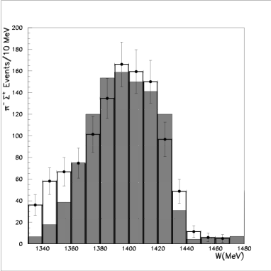
Figure 3: Event distribution in the region of the $\Lambda(1405)$ for set I (shaded area) in comparison to the data from [36].

We finally discuss the poles in the complex energy plane for the different Riemann sheets. In discussing the $\Lambda(1405)$ resonance the closest thresholds are the ones corresponding to the $\pi\Sigma$ and $\bar{K}N$ states. Hence, one has to consider generally four sheets. The physical one labelled by $(+,+)$, the second $(-,+)$, the third $(-,-)$ and the fourth sheet $(+,-)$. The signs inside the brackets refer to the sign ambiguity present in the definition of the modulus of the c.m. three–momentum for the channels $\pi\Sigma$ and $\bar{K}N$, respectively. In this way, the ‘$+$’ sign indicates that the imaginary part of the modulus of the three–momentum is always positive in the whole $s$–plane and the ‘$-$’ sign refers to the contrary (unphysical sheet). When looking at the pole structure in the unphysical Riemann sheets one realizes the presence of three poles corresponding to the three expected neutral members of a $J^{P}=\frac{1}{2}^{-}$ baryon nonet (in the isospin limit, two of them with $I=0$ and another one with $I=1$). We also find that the pole positions change appreciably from one sheet to the other, which is a clear indication of a large meson–baryon component. For the second and third sheets, which are the closest ones to the physical sheet, we have the following pole positions. Sheet II: $(1379.2-i\,27.6)\,$MeV, $(1433.7-i\,11.0)\,$MeV ($I=0$) and $(1444.0-i\,69.4)\,$MeV ($I=1$). Sheet III: $(1346.2-i\,3.0)\,$MeV and $(1411.9-i\,48.8)\,$MeV ($I=0)$ and $(1419.0-i\,41.7)\,$MeV ($I=1$). Note that the $\Lambda(1405)$ resonance is described by two poles on sheets II and III with rather different imaginary parts indicating a clear departure from the Breit-Wigner situation for this resonance as already stated long time ago, see e.g. refs. [36, 37]. It is also worth to remark the presence of another pole with $I=0$ very close to the threshold of the $\pi\Sigma$ states with a mass inside the range of energies covered by fig.3. In addition, since we have seen that the resulting value of the subtraction constant can easily be explained as coming from a cut–off with a natural value, one should conclude that, at least, this set of poles largely corresponds to meson–baryon resonances. However, one should include explicit resonance fields (which can be straightforwardly done in this approach) in order to finally assess the absence or the presence of small preexisting baryon resonance components in their wave functions, analogously as it has been done in the meson–meson sector in refs.[38, 21]. Finally, the $S=0$ [39, 40] and $S=-2$ S-wave meson–baryon amplitudes should be studied analogously in order to complete the assignment of resonances belonging to the aforementioned $\frac{1}{2}^{-}$ baryon nonet.

6. We have derived a general and systematic method to resum the right–hand cut contributions from a perturbative (chiral) series. This method should be applied whenever these contributions become far from being perturbative both in the low (or higher) energy regimes, as for instance in the S–wave kaon–nucleon interactions for strangeness $S=-1$ as discussed in detail here. The theory can be seen as a reformulation in more general terms of the approach already applied to study the meson–meson scattering in refs.[21, 38, 41]. Dispersion relations are used to perform the necessary resummation of the chiral perturbation theory amplitudes given at any order. These CHPT amplitudes are then incorporated in our general expressions for the partial wave amplitudes by requiring the matching between both results in a well defined chiral power counting. Here, we have simply considered the lowest order (tree level) CHPT approximation as our starting point. A good description of the scattering data in the $K^{-}p$, $\pi\Sigma$ and $\pi\Lambda$ channels as well as for the threshold branching ratios is obtained. In addition, we have given an improved theoretical prescription to calculate the $\Sigma\pi$ event distributions in the region of the $\Lambda(1405)$ leading to a good reproduction of the data. We have also discussed the pole structure in that energy region. In the future, one should extend these considerations in three ways. First, a second or third order (relativistic) CHPT amplitude should be used as input and higher partial waves should be included. Second, one should consider other strangeness channels (in particular $\pi N$ scattering has to be treated systematically, see [18]) and also include explicit resonance fields (as it is possible in this framework). This is of particular interest for the question whether the $\Lambda(1405)$ is a pure meson–baryon boundstate or has a small “preexisting” component. Third, the extension to electromagnetic kaon production off nucleons is of interest due to the data from ELSA and TJNAF.

Acknowledgements

The work of J.A.O. was supported in part by funds from DGICYT under contract PB96-0753 and from the EU TMR network Eurodaphne, contract no. ERBFMRX-CT98-0169.

References

- [1] J. Gasser, M. E. Sainio and A. Svarc, Nucl. Phys. B307 (1988) 779.
- [2] E. Jenkis and A. V. Manohar, Phys. Lett. B255 (1991) 558.
- [3] V. Bernard, N. Kaiser, J. Kambor and Ulf-G. Meißner, Nucl. Phys. B388 (1992) 315.
- [4] V. Bernard, N. Kaiser and Ulf-G. Meißner, Int. J. Mod. Phys. E4 (1995) 193.
- [5] P.J. Ellis and H.-B. Tang, Phys. Rev. C57 (1998) 3356.
- [6] T. Becher and H. Leutwyler, Eur. Phys. J. C9 (1999) 643.
- [7] S. Weinberg, Phys. Lett. B251 (1990) 288.
- [8] C.-H. Lee, G.E. Brown, D.P. Min and M. Rho, Nucl. Phys. A585 (1995) 401.
- [9] M. Savage, Phys. Lett. B331 (1994) 411.
- [10] N. Kaiser, P.B. Siegel and W. Weise, Nucl. Phys. A594 (1995) 325.
- [11] E. Oset and A. Ramos, Nucl. Phys. A635 (1998) 99.
- [12] J. Gasser and Ulf-G. Meißner, Nucl. Phys. B357 (1991) 90.
- [13] J. Kambor, C. Wiesendanger and D. Wyler, Nucl. Phys. B465 (1996) 215.
- [14] A.V. Anisovich and H. Leutwyler, Phys. Lett. B375 (1996) 335.
- [15] M.F.M. Lutz and E.E. Kolomeitsev, nucl-th/0004021.
- [16] P.B. Siegel and W. Weise, Phys. Rev. C38 (1988) 2221.
- [17] A. Müller-Groeling, K. Holinde and J. Speth, Nucl. Phys. A513 (1990) 557.
- [18] Ulf-G. Meißner and J.A. Oller, Nucl. Phys. A673 (2000) 311.
- [19] P.G. Ratcliffe, Phys. Rev. D59 (1999) 014038.
- [20] V. Bernard, N. Kaiser and Ulf-G. Meißner, Nucl. Phys. B364 (1991) 283.
- [21] M. Jamin, J.A. Oller and A. Pich, Nucl. Phys. B587 (2000) 331.
- [22] S. Descotes and J. Stern, Phys. Lett. B488 (2000) 274.
- [23] J. Gasser and H. Leutwyler, Nucl. Phys. B250 (1985) 517.
- [24] Ulf-G. Meißner and J.A. Oller, Nucl. Phys. A679 (2001) 671, hep-ph/0005253.
- [25] W. E. Humphrey and R. R. Ross, Phys. Rev. 127 (1962) 1305.
- [26] J. K. Kim, Phys. Rev. Lett. 14 (1965) 29.
- [27] M. Sakitt et al., Phys. Rev. 139 (1965) B719.
- [28] W. Kittel, G. Otter and I. Wacek, Phys. Lett. 21 (1966) 349.
- [29] D. Evans et al., J. Phys. G9 (1983) 885.
- [30] J. Ciborowski et al., J. Phys. G8 (1982) 13.
- [31] R. Novak et al., Nucl. Phys. B139 (1978) 61.
- [32] D. Tovee et al, Nucl. Phys. B33 (1971) 493.
- [33] M. Iwasaki et al., Phys. Rev. Lett. 78 (1997) 3067.
- [34] A.D. Martin, Nucl. Phys. B179 (1981) 33.
- [35] B.R. Martin, Nucl. Phys. B94 (1975) 413.
- [36] R.J. Hemingway, Nucl. Phys B253 (1985) 742.
- [37] R.H. Dalitz and A. Deloff, J. Phys. G17 (1991) 289.
- [38] J.A. Oller and E. Oset, Phys. Rev. D60 (1999) 074023.
- [39] N. Kaiser, P.B. Siegel and W. Weise, Phys. Lett. B362 (1995) 23.
- [40] J.C. Nacher, A. Parreno, E. Oset, A. Ramos, A. Hosaka and M. Oka, Nucl. Phys. A678 (2000) 187.
- [41] J.A. Oller, Phys. Lett. B477 (2000) 187.