UWThPh-2000-43

October 2000

STRONG INTERACTIONS
OF LIGHT FLAVOURS

Gerhard Ecker

Institut für Theoretische Physik, Universität Wien

Boltzmanngasse 5, A–1090 Wien, Austria

After an introduction to chiral perturbation theory, the effective field theory of the standard model at low energies, a brief overview is given of applications to light-flavour physics. Three topics in the strong interactions of pseudoscalar mesons are then discussed in some detail: loops and chiral logs, pion-pion scattering and isospin violation.

Lectures given at the

Advanced School on QCD 2000, Benasque, Spain

July 3 - 6, 2000

To appear in the Proceedings

Work supported in part by TMR, EC-Contract No. ERBFMRX-CT980169 (EURODA$\Phi$NE).

1 Chiral Perturbation Theory

1.1 Introduction

The physics of light flavours at low energies can be described in the framework of chiral perturbation theory (CHPT) [1, 2, 3, 4]. It is a typical example of an effective field theory:

• The domain of validity of CHPT is restricted to the confinement regime of QCD, i.e., to energies below some typical scale $\Lambda$ of the order of $M_{\rho}$.

• The matching of CHPT to the underlying standard model is a difficult nonperturbative problem: neither CHPT nor QCD can be treated perturbatively at $E=\Lambda$. The challenge consists in bridging the gap between the perturbatively accessible domains of both theories:

  CHPT	$\leftrightarrow$	perturbative QCD
  $E<M_{\rho}$		$E>1.5$ GeV

• The difficulty of matching the two theories is related to the existence of a phase transition. The degrees of freedom of the two quantum field theories are completely different: quarks and gluons on the one hand, hadrons, in particular the pseudoscalar mesons as the lightest ones, on the other hand.

• Symmetries are the main input for the construction of CHPT, especially the spontaneously (and explicitly) broken chiral symmetry of QCD. This ensures compatibility with the underlying standard model but also leaves considerable freedom for the effective Lagrangians. The abundance of free parameters, the so-called low-energy constants (LECs), becomes especially acute at higher orders in the low-energy expansion. Additional input is necessary to get information on those constants. The most promising approaches rely on the large-$N_{c}$ expansion (e.g., Refs. [5, 6]) and on lattice QCD (the most recent reference is [7]).

1.2 Chiral symmetry

The starting point of CHPT is QCD in a purely theoretical setting, the chiral limit with $N_{f}=$ 2 or 3 massless quarks $u,d~{}[,s]$. In this limit, the QCD Lagrangian ${\cal L}^{0}_{\rm QCD}$ exhibits a global symmetry

$$\underbrace{SU(N_{f})_{L}\times SU(N_{f})_{R}}_{\mbox{chiral group $G$}}\times U(1)_{V}\times U(1)_{A}~{}.$$

$U(1)_{V}$ is realized as baryon number in CHPT. The axial $U(1)_{A}$ is not a symmetry at the quantum level due to the Abelian anomaly (see Ref. [8] for a recent treatment in the chiral framework).

There is strong evidence both from phenomenology and from theory that chiral symmetry is spontaneously broken (see Ref. [9] for more details and references to the original work):

$$G\longrightarrow H=SU(N_{f})_{V}~{},$$ (1.1)

with the conserved subgroup $H$ either isospin ($N_{f}=2$) or flavour $SU(3)$ ($N_{f}=3$).

What is the underlying mechanism for this spontaneous breakdown ? In a standard proof of the Goldstone theorem [10] one starts from the charge operator in a finite volume $V$, $Q^{V}=\int_{V}d^{3}xJ^{0}(x)$ and assumes the existence of a (sufficiently local) operator $A$ such that the following order parameter is nonvanishing:

$$\lim_{V\rightarrow\infty}\langle 0|[Q^{V}(x^{0}),A]|0\rangle\neq 0~{}.$$ (1.2)

The Goldstone theorem then tells us that there exists a massless state $|GB\rangle$ with

$$\langle 0|J^{0}(0)|GB\rangle\langle GB|A|0\rangle\neq 0~{}.$$ (1.3)

The relation (1.3) contains two nonvanishing matrix elements. The first one involves only the symmetry current and it is therefore independent of the specific order parameter:

$$\langle 0|J^{0}(0)|GB\rangle\neq 0$$ (1.4)

is a necessary and sufficient condition for spontaneous breaking. In QCD, this matrix element is determined by the meson decay constant $F$, the chiral limit value of $F_{\pi}=92.4$ MeV.

Which then is the order parameter of chiral symmetry breaking in QCD ? Since the spontaneously broken currents are axial, $A$ in (1.2) must be a pseudoscalar, colour singlet operator. The unique choice for local operators in QCD with lowest operator dimension three is

$$A_{i}=\overline{q}\gamma_{5}\lambda_{i}q$$ (1.5)

with

$$\left[Q^{i}_{A},A_{j}\right]=-\displaystyle\frac{1}{2}\overline{q}\{\lambda_{i},\lambda_{j}\}q~{}.$$ (1.6)

If the vacuum is invariant under $SU(N_{f})_{V}$,

$$\langle 0|\overline{u}u|0\rangle=\langle 0|\overline{d}d|0\rangle\left[=\langle 0|\overline{s}s|0\rangle\right]~{}.$$ (1.7)

Therefore, a nonvanishing quark condensate

$$\langle 0|\overline{q}q|0\rangle\neq 0$$ (1.8)

is sufficient for spontaneous chiral symmetry breaking, but certainly not necessary. Increasing the operator dimension, the next candidate is the so–called mixed condensate of dimension five ($\langle 0|\overline{q}\sigma_{\mu\nu}\lambda_{\alpha}qG^{\alpha\mu\nu}|0\rangle\neq 0$), and there are many more possibilities for operator dimensions $\geq 6$. Although all order parameters are in principle equally good for triggering the Goldstone mechanism one may expect a special role for the quark condensate as the dominant order parameter of spontaneous chiral symmetry breaking.

It has recently been argued that the answer could depend crucially on $N_{f}$ because there are indications for $\langle 0|\overline{q}q|0\rangle$ decreasing with $N_{f}$ [11, 12]. As I will point out later on, the Gell-Mann–Okubo mass formula for the pseudoscalar mesons supports a large quark condensate for $N_{f}=3$. If the condensate indeed increases for smaller $N_{f}$, the dominance should be all the more pronounced in the two-flavour case. As a matter of fact, recent developments in $\pi\pi$ scattering (see Sec. 4) leave little doubt about the dominant order parameter for $N_{f}=2$.

1.3 Chiral Lagrangians

Spontaneously broken symmetries are realized nonlinearly on the Goldstone boson fields of which there are dim $G/H=N_{f}^{2}-1$ in the case of chiral symmetry: the pions for $N_{f}=2$, with kaons and the $\eta$ meson in addition for $N_{f}=3$. This nonlinear realization is implemented by matrix fields (usually in the fundamental representation) $u_{L}(\phi),u_{R}(\phi)$ that parametrize the coset space $G/H$ in terms of the Goldstone fields $\phi$. Chiral transformations $g=(g_{L},g_{R})\in G$ are realized as

$$u_{A}(\phi)\stackrel{{\scriptstyle g}}{{\longrightarrow}}g_{A}u_{A}(\phi)h(g,\phi)^{-1}\qquad(A=L,R)$$ (1.9)

with a so-called compensator (field) $h(g,\phi)\in SU(N_{f})_{V}$. Its dependence on the fields $\phi$ is a characteristic feature of the nonlinear realization.

In the purely mesonic sector, the Goldstone fields are usually parametrized in terms of another matrix field $U(\phi)$ that transforms linearly under chiral transformations:

$$U(\phi):=u_{R}(\phi)u_{L}(\phi)^{\dagger}\stackrel{{\scriptstyle g}}{{\longrightarrow}}g_{R}U(\phi)g_{L}^{-1}~{}.$$ (1.10)

The nonlinear realization of $G$ on $\phi$ implies that the matrix $U(\phi)$ cannot be a polynomial function of $\phi$. One standard choice is the exponential parametrization with

$$u_{R}(\phi)=u_{L}(\phi)^{\dagger}:=u(\phi)=\exp{i\lambda_{a}\phi^{a}/2F}$$ (1.11)

$$\longrightarrow\qquad U(\phi)=u(\phi)^{2}$$

where $F$ is defined by the Goldstone matrix element :

$$\langle 0|\overline{q(x)}\gamma^{\mu}\gamma_{5}\frac{\lambda_{a}}{2}q(x)|\phi_{b}(p)\rangle=i\delta_{ab}Fp^{\mu}e^{-ipx}~{}.$$ (1.12)

As chiral Lagrangians are built from the matrix fields $u_{L,R}$ or $U$ it is clear that the corresponding quantum field theories are generically nonrenormalizable.

It is now time to take leave from the theorist’s world of chiral symmetry and admit that there is no chiral symmetry in nature. In the standard model, chiral symmetry is explicitly broken in two different ways:

1. Nonvanishing quark masses: this is expected to be a small deviation from the chiral limit for two flavours but less so for $N_{f}=3$.

2. Electroweak interactions: these can be taken into account perturbatively in $\alpha$ and $G_{F}$ (more about this in Sec. 2).

The main assumption underlying CHPT is that an expansion around the chiral limit is a meaningful approximation. Even neglecting the electroweak interactions, i.e., for $\alpha=G_{F}=0$, CHPT is from the outset based on a two-fold expansion, both in the momenta of pseudoscalar mesons and in the quark masses. For the effective chiral Lagrangian ${\cal L}_{\rm eff}$, this implies

$${\cal L}_{\rm eff}=\sum_{i,j}{\cal L}_{ij}~{},\qquad{\cal L}_{ij}=O(\partial^{i}m^{j}_{q})$$ (1.13)

where $\partial$ stands for a derivative.

The two expansions can be related to each other by making use of the relation between meson and quark masses:

$$M_{M}^{2} \sim Bm_{q}+O(m_{q}^{2})$$ (1.14)

$$B = -\langle 0|\overline{u}u|0\rangle/F^{2}~{}.$$

Depending on the value of the quark condensate, two different schemes have been considered.

A. Standard CHPT

This is the original scheme [1, 2, 3] where the terms linear in the quark masses are assumed to dominate the meson masses in (1.14). This corresponds to a value of $B(\nu=1~{}\rm GeV)\sim$ 1.4 GeV ($\nu$ is the QCD renormalization scale) and gives rise to the standard values of light quark mass ratios. It also implies the Gell-Mann–Okubo mass formula $3M^{2}_{\eta_{8}}=4M_{K}^{2}-M_{\pi}^{2}$ at lowest order in the chiral expansion. The standard chiral counting is

$$m_{q}=O(M^{2})=O(p^{2})~{},$$ (1.15)

implying in turn

$${\cal L}_{\rm eff}=\sum_{n}{\cal L}_{n}~{},\qquad{\cal L}_{n}=\sum_{i+2j=n}{\cal L}_{ij}~{}.$$ (1.16)

Generalized CHPT

The proponents of the second scheme ([13] and references therein) allow for the possibility that $B$ is much smaller, e.g., $B(\nu=1{\rm~{}GeV})=O(F_{\pi})$. In this case,

$$M_{M}^{2}\sim O(m_{q}^{2})$$ (1.17)

and the light quark mass ratios would be quite different from the standard values. The more natural chiral counting is $m_{q}=O(p)$ now and the (same) effective Lagrangian is reordered, with more terms catalogued at lower orders than in the standard expansion. The obvious drawback is that there are more unknown LECs at any given order. For instance, the Gell-Mann–Okubo mass formula is not a consequence of Generalized CHPT. It is therefore rather comforting that there is at present no compelling evidence for scheme B. On the other hand, it is difficult to prove the validity of scheme A, especially for three light flavours. I will come back in Sec. 4 to the situation in the two-flavour case where evidence for the standard procedure has been mounting recently.

To construct the effective chiral Lagrangian(s), we follow the procedure of Gasser and Leutwyler [2, 3] by coupling external matrix fields $v_{\mu},a_{\mu},s,p$ to the quarks:

$${\cal L}^{0}_{\rm QCD}\to{\cal L}^{0}_{\rm QCD}+\overline{q}\gamma^{\mu}(v_{\mu}+a_{\mu}\gamma_{5})q-\overline{q}(s-ip\gamma_{5})q~{}.$$ (1.18)

Chiral symmetry is promoted to a local symmetry in this way. QCD Green functions and amplitudes at low energies can then be calculated from a quantum field theory with the most general effective Lagrangian that respects this local chiral symmetry [4].

In the standard scheme, this effective chiral Lagrangian for the strong interactions of pseudoscalar mesons takes the general form

$${\cal L}_{\rm eff}={\cal L}_{2}+{\cal L}_{4}+{\cal L}_{6}+\dots$$ (1.19)

The lowest-order Lagrangian ${\cal L}_{2}$ of $O(p^{2})$ is given by

$${\cal L}_{2}=\frac{F^{2}}{4}\langle D_{\mu}UD^{\mu}U^{\dagger}+\chi U^{\dagger}+\chi^{\dagger}U\rangle$$ (1.20)

with a gauge-covariant derivative $D_{\mu}U=\partial_{\mu}U-i(v_{\mu}+a_{\mu})U+iU(v_{\mu}-a_{\mu})$ and with $\chi=2B(s+ip)$. The two free parameters $F,B$ are related to the pion decay constant and to the quark condensate, respectively:

$$F_{\pi} = F\left[1+O(m_{q})\right]$$ (1.21)

$$\langle 0|\overline{u}u|0\rangle = -F^{2}B\left[1+O(m_{q})\right]~{}.$$

CHPT at lowest order amounts to the calculation of Green functions and amplitudes with ${\cal L}_{2}$ at tree level where one sets all external fields to zero at the end except for

$$s(x)={\rm diag}(m_{u},m_{d}[,m_{s}])$$ (1.22)

to account for the explicit chiral symmetry breaking through the quark masses. The results are equivalent to the current algebra amplitudes of the sixties. Amplitudes depend only on $F_{\pi}$ and $M_{M}$, e.g., the Weinberg amplitude [14] for pion-pion scattering:

$$A_{2}(s,t,u)=\frac{s-M_{\pi}^{2}}{F_{\pi}^{2}}~{}.$$ (1.23)

It is remarkable that one seems to get an absolute prediction from pure symmetry only! The skeptic will soon realize that it is in fact a relation between a four-point function and the two-point function (1.12), which is only possible for a nonlinearly realized symmetry.

At next-to-leading order in the chiral expansion, the chiral Lagrangian ${\cal L}_{4}$ contains 7 (10) measurable LECs for $N_{f}=$ 2 (3) [2, 3]. At this point, we have to take the quantum field theory character of CHPT serious. Since ${\cal L}_{\rm eff}$ is hermitian tree amplitudes are real. On the other hand, unitarity and analyticity demand complex amplitudes in general. For instance, the partial-wave amplitudes in $\pi\pi$ scattering (cf. Sec. 4) satisfy

$$\mbox{\rm Im}t^{I}_{l}(s)\geq(1-\displaystyle\frac{4M_{\pi}^{2}}{s})^{\frac{1}{2}}|t^{I}_{l}(s)|^{2}~{}.$$ (1.24)

The Weinberg amplitude (1.23) produces (real) partial waves $t^{I}_{l}(s)$ of $O(p^{2})$ (for $l\leq 1$). Thus, the scattering amplitude must have a nonvanishing imaginary part, starting at $O(p^{4})$.

A systematic low-energy expansion to $O(p^{n})$ requires therefore a concurrent loop expansion for $n>2$. Since CHPT loop amplitudes are at least as divergent as in renormalizable quantum field theories, the theory has to be regularized and renormalized. Renormalization is essential for getting cutoff independent results. The procedure amounts to absorbing divergences by the coupling constants in ${\cal L}_{4},{\cal L}_{6},\dots$ rendering the observable LECs scale dependent at the same time. This scale dependence is by construction always compensated by the scale dependence of loop amplitudes.

The LECs contain the effect of all those (heavy) degrees of freedom that do not appear as explicit fields in ${\cal L}_{\rm eff}$. For instance, the effective Lagrangian for $N_{f}=2$ contains only pions. Kaons and the $\eta$ enter only via the coupling constants. For $N_{f}=3$, the dominant degrees of freedom governing the size of LECs are the meson resonances [15].

2 Survey of Applications

Before discussing a few selected examples in some detail, I want to give a brief overview of the rapidly growing field of applications of CHPT. One way to summarize the current status is to present the effective chiral Lagrangian of the standard model in Table 1.

Table 1: The effective chiral Lagrangian of the Standard Model

${\cal L}_{\rm chiral\;order}$  ($\#$ of LECs)	loop  order
${\cal L}_{p^{2}}(2)$+${\cal L}_{p^{4}}^{\rm odd}(0)$+ ${\cal L}_{G_{F}p^{2}}^{\Delta S=1}(2)$ +${\cal L}_{e^{2}p^{0}}^{\rm em}(1)$ +${\cal L}_{G_{8}e^{2}p^{0}}^{\rm emweak}(1)$	$L=0$
+ ${\cal L}_{p}^{\pi N}(1)$+${\cal L}_{p^{2}}^{\pi N}(7)$ +${\cal L}_{G_{8}p^{0}}^{MB,\Delta S=1}(2)$+ ${\cal L}_{G_{8}p}^{MB,\Delta S=1}(8)$ + ${\cal L}_{e^{2}p^{0}}^{\pi N,{\rm em}}(3)$
+ $\underline{{\cal L}_{p^{4}}^{\rm even}(10)}$+ $\underline{{\cal L}_{p^{6}}^{\rm odd}(32)}$ +$\underline{{\cal L}_{G_{8}p^{4}}^{\Delta S=1}(22)}$ +$\underline{{\cal L}_{e^{2}p^{2}}^{\rm em}(14)}$ + $\underline{{\cal L}_{G_{8}e^{2}p^{2}}^{\rm emweak}(14)}$	$L=1$
+ $\underline{{\cal L}_{e^{2}p}^{\rm leptons}(5)}$
+ $\underline{{\cal L}_{p^{3}}^{\pi N}(23)}$+ $\underline{{\cal L}_{p^{4}}^{\pi N}(114)}$ + $\underline{{\cal L}_{G_{8}p^{2}}^{MB,\Delta S=1}(?)}$ +$\underline{{\cal L}_{e^{2}p}^{\pi N,{\rm em}}(8)}$
+ $\underline{{\cal L}_{p^{6}}^{\rm even}(90)}$	$L=2$

The various Lagrangians are ordered by their chiral dimension, with the number of independent LECs shown in brackets. Except for the pieces with superscript $\pi N$, the numbers refer to $N_{f}=3$. The fully renormalized Lagrangians are underlined. This means that the divergence structure of the corresponding loop functionals is explicitly known in a process independent manner.

The Table indicates that CHPT is not restricted to the pseudoscalar mesons only (Lagrangians ${\cal L}_{p^{2}}(2)$, ${\cal L}_{p^{4}}^{\rm odd}(0)$, ${\cal L}_{p^{4}}^{\rm even}(10)$, ${\cal L}_{p^{6}}^{\rm odd}(32)$ and ${\cal L}_{p^{6}}^{\rm even}(90)$). The inclusion of baryons is straightforward but there are substantial differences to the purely mesonic case:

• Baryons are not Goldstone modes: there are no “soft” baryons. Their interactions are less constrained by chiral symmetry.

• In the presence of baryons, the effective Lagrangian has parts of every integer chiral order even in the standard scheme:

  $${\cal L}_{\rm eff}=\sum_{n=1,2,3,\dots}{\cal L}_{n}~{}.$$ (2.1)

  Compared to the purely mesonic case with $n=2,4,6,\dots$, the chiral expansion progresses much more slowly.

• Baryon resonances are often closer to threshold than in the case of mesons ($\Delta$ vs. $\rho$). This limits the domain of validity of the chiral expansion.

• The baryon mass $m$ complicates the chiral counting because it does not vanish in the chiral limit. The traditional method is called Heavy Baryon CHPT [16] and it amounts to shifting the baryon mass from the propagators to the vertices of an effective Lagrangian. The method is systematic and straightforward but it does not converge in some kinematic configurations. Therefore, an alternative called Relativistic Baryon CHPT has recently been put forward [17] that is manifestly Lorentz invariant at every step and does not have the deficiency of HBCHPT. Loop calculations and the regularization procedure are somewhat more involved. Both approaches have been applied to a variety of processes, albeit most of them only in HBCHPT so far. The corresponding Lagrangians in Table 1 are ${\cal L}_{p}^{\pi N}(1)$, ${\cal L}_{p^{2}}^{\pi N}(7)$, ${\cal L}_{p^{3}}^{\pi N}(23)$ and ${\cal L}_{p^{4}}^{\pi N}(114)$.

• Table 1 is restricted to single-baryon processes. It does not account for applications of chiral methods in nuclear physics such as in nucleon-nucleon scattering (see Ref. [18] for a review of recent developments in this field).

Other heavy fields can also be included in the effective Lagrangians, although at the expense of possible double counting in some cases, e.g., the meson and baryon resonances.

So far, I have only considered strong interactions. Electroweak interactions can be incorporated perturbatively in $G_{F}$ and $\alpha$. The previous method of constructing effective chiral Lagrangians has to be extended in this case. To describe the nonleptonic weak interactions of mesons treated by Hans Bijnens in his lectures [6], one first has to integrate out the heavy fields $W,t,b,c$ to obtain an effective Hamiltonian for $\Delta S=1$ nonleptonic weak interactions. The task is then to construct the most general effective chiral Lagrangian with the same chiral transformation properties as this effective Hamiltonian. The corresponding Lagrangians in Table 1 are ${\cal L}_{G_{F}p^{2}}^{\Delta S=1}(2)$, ${\cal L}_{G_{8}p^{4}}^{\Delta S=1}(22)$ for mesons only and ${\cal L}_{G_{8}p^{0}}^{MB,\Delta S=1}(2)$, ${\cal L}_{G_{8}p}^{MB,\Delta S=1}(8)$, ${\cal L}_{G_{8}p^{2}}^{MB,\Delta S=1}(?)$ for baryons and mesons.

Inclusion of the electromagnetic interactions is still a little more involved, being nonlocal at low energies. One introduces the dynamical photon with the proper kinetic term (and gauge fixing) and an additional chiral Lagrangian that transforms like a product of two electromagnetic currents. The corresponding Lagrangians are ${\cal L}_{e^{2}p^{0}}^{\rm em}(1)$, ${\cal L}_{e^{2}p^{2}}^{\rm em}(14)$ (mesons) and ${\cal L}_{e^{2}p^{0}}^{\pi N,{\rm em}}(3)$, ${\cal L}_{e^{2}p}^{\pi N,{\rm em}}(8)$ (baryons and mesons). The combination of nonleptonic weak and electromagnetic interactions requires still another set of Lagrangians that have only been considered for mesons so far : ${\cal L}_{G_{8}e^{2}p^{0}}^{\rm emweak}(1)$, ${\cal L}_{G_{8}e^{2}p^{2}}^{\rm emweak}(14)$.

Finally, leptons can also be incorporated as explicit fields in the effective Lagrangian, up to now again with mesons only: ${\cal L}_{e^{2}p}^{\rm leptons}(5)$.

Instead of trying to give proper credit to all the work related to the effective Lagrangians in Table 1, I refer to some recent workshops from where up-to-date information can be recovered [19, 20, 21].

3 Loops and Chiral Logs

3.1 Loop expansion

Successive orders in the chiral expansion can be characterized by the chiral dimension $D_{L}$ defined as the degree of homogeneity of amplitudes in external momenta and meson masses. In the meson sector with the standard chiral counting, a generic $L$-loop diagram with $N_{n}$ vertices from the Lagrangian ${\cal L}_{n}~{}(n=2,4,6,\dots)$ and $I$ internal lines has $D_{L}=4L+\sum_{n\geq 2}nN_{n}-2I$. The topological relation $L=I-\sum_{n}N_{n}+1$ for connected diagrams leads to the final expression [1]

$$D_{L}=2L+2+\sum_{n\geq 4}(n-2)N_{n}\geq 2L+2~{}.$$ (3.1)

As $D_{L}$ increases with $L$ while the physical dimension of a given amplitude remains fixed, each loop comes with a factor $1/(4\pi F)^{2}$ so that the chiral expansion is really an expansion in

$$\frac{p^{2}}{(4\pi F_{\pi})^{2}}=0.18\frac{p^{2}}{M_{K}^{2}}~{}.$$ (3.2)

Corrections of the order of 20% are therefore to be expected in the three-flavour case. For $N_{f}=2$, one may limit the expansion to smaller momenta with correspondingly improved precision.

The state of the art for the strong interactions of mesons is $O(p^{6})$. The possible values of $L$ and $N_{n}$ ($n=4,6$) in (3.1) for $D_{L}=6$ are shown graphically in Fig. 1 as so-called skeleton diagrams. For actual calculations to $O(p^{6})$, I refer again to the workshops listed in Refs. [19, 20, 21].

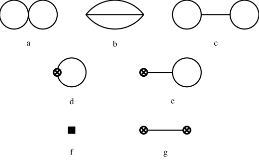
Figure 1: Skeleton diagrams of $O(p^{6})$. Propagators and vertices carry the full tree structure associated with the lowest-order Lagrangian ${\cal L}_{2}$. Normal vertices are from ${\cal L}_{2}$, crossed circles and the full square denote vertices from ${\cal L}_{4}$ and ${\cal L}_{6}$, respectively.

The renormalization procedure is best carried out in a process independent way via the divergent part of the generating functional of Green functions. Such an approach has several advantages:

• It provides a nontrivial check for all explicit loop calculations for specific processes.

• It produces renormalization group equations for the renormalized, scale-dependent LECs.

• As an important byproduct, one gets the leading infrared singularities for free, the so-called chiral logs.

3.2 Renormalization at $O(p^{4})$

In dimensional regularization, divergences appear in the combination

$$\frac{\mu^{d-4}}{(4\pi)^{2}}\left[\frac{1}{d-4}+\frac{1}{2}\ln{M^{2}/\mu^{2}}+\dots\right]$$ (3.3)

that is independent of the arbitrary renormalization scale $\mu$. $M$ denotes a typical scale, e.g., $M_{\pi}$ ($M_{K}$) for $N_{f}=$ 2 (3). Renormalization consists in splitting the coupling constants $L_{i}$ of the Lagrangian ${\cal L}_{4}$ in an analogous fashion :

$$L_{i}=\mu^{d-4}\left[\frac{\Gamma_{i}}{(4\pi)^{2}(d-4)}+\underbrace{L_{i}^{r}(\mu)}_{{\rm ren.~{}LEC}}+\dots\right]~{}.$$ (3.4)

The coefficients $\Gamma_{i}$ are chosen such that the divergences of one-loop Green functions are cancelled by the tree-level contributions from ${\cal L}_{4}$. As a consequence, physical amplitudes depend on the scale-independent combinations

$$L_{i}^{r}(\mu)-\frac{1}{2}\Gamma_{i}l$$ (3.5)

with the chiral log

$$l=\frac{1}{(4\pi)^{2}}\ln{M^{2}/\mu^{2}}~{}.$$

Scale independence of these combinations implies renormalization group equations for the measurable LECs $L_{i}^{r}(\mu)$ :

$$\mu\frac{dL_{i}^{r}(\mu)}{d\mu} = -\frac{\Gamma_{i}}{(4\pi)^{2}}$$ (3.6)

$$\to\qquad L_{i}^{r}(\mu_{2}) = L_{i}^{r}(\mu_{1})+\frac{\Gamma_{i}}{16\pi^{2}}\ln\frac{\mu_{1}}{\mu_{2}}~{}.$$

The phenomenological values of the LECs for $N_{f}=3$ are shown in Table 2. Some of them have recently been reevaluated on the basis of an $O(p^{6})$ analysis [22].

Table 2: Phenomenological values of $L^{r}_{i}(M_{\rho})$

i	$L^{r}_{i}(M_{\rho})\times 10^{3}$
	1995                   2000		main source
	(Amoros et al. [22])
1	0.4 $\pm$ 0.3	0.52 $\pm$ 0.23	$K_{e4},(\pi\pi\to\pi\pi)$
2	1.35 $\pm$ 0.3	0.72 $\pm$ 0.24	$K_{e4},(\pi\pi\to\pi\pi)$
3	$-$3.5 $\pm$ 1.1	$-$2.70 $\pm$ 0.99	$K_{e4},(\pi\pi\to\pi\pi)$
4	$-$0.3 $\pm$ 0.5		Zweig rule
5	1.4 $\pm$ 0.5	0.65 $\pm$ 0.12	$F_{K}/F_{\pi}$
6	$-$0.2 $\pm$ 0.3		Zweig rule
7	$-$0.4 $\pm$ 0.2	$-$0.26 $\pm$ 0.15	Gell-Mann–Okubo,
			$L_{5},L_{8}$
8	0.9 $\pm$ 0.3	0.47 $\pm$ 0.18	$M_{K^{0}}-M_{K^{+}},L_{5}$
9	6.9 $\pm$ 0.7		$\langle r^{2}\rangle^{\pi}_{V}$
10	$-$5.5 $\pm$ 0.7		$\pi\rightarrow e\nu\gamma$

3.3 Renormalization at $O(p^{6})$

The procedure here is similar, albeit more complicated than before due to the presence of loop diagrams with $L\leq 2$. Let us first have a look at the reducible diagrams c,e,g in Fig. 1. One expects that the sum of these diagrams is finite (and scale independent) because the one-loop renormalization has already been carried out. This is in fact true, but only with an additional technical requirement that would not occur in renormalizable quantum field theories: the Lagrangian ${\cal L}_{4}$ has to be chosen appropriately [23].

Turning to the irreducible diagrams a,b,d in Fig. 1, general theorems of renormalization theory tell us that the divergences must be polynomials in masses and external momenta of $O(p^{6})$. This is a highly nontrivial constraint on the procedure because each type of diagrams a,b,d separately has in addition nonlocal divergences. For instance, diagrams a and d involve the Green function $G(x,x)$ (and derivatives):

$$G(x,x)=\frac{2\mu^{d-4}}{(4\pi)^{2}}\left(\frac{1}{d-4}+\frac{1}{2}\ln{M^{2}/\mu^{2}}\right)a_{1}(x,x)+\underbrace{\overline{G}(x,x)}_{\rm finite,nonlocal}~{},$$ (3.7)

with $a_{1}(x,x)$ a (local) Seeley-DeWitt coefficient. Therefore, diagrams a,b and d separately have nonlocal divergences of the form

$$\frac{1}{d-4}\overline{G}(x,x)\quad{\rm and}\quad\frac{1}{d-4}\ln{M^{2}/\mu^{2}}$$ (3.8)

that have to cancel in the sum. As already emphasized, this requirement is a very efficient check on the correctness of the renormalization procedure [23].

The remaining divergences are indeed polynomials in masses and derivatives (momenta) of $O(p^{6})$. Those divergences are canceled by the divergent parts of the LECs of $O(p^{6})$ in the tree-level amplitudes characterized by the vertex f in Fig. 1. The corresponding effective Lagrangian has the general form [24]

$${\cal L}_{6}=\sum_{i=1}^{53(90)}\underbrace{C_{i}}_{\rm coeffs.}\underbrace{O_{i}}_{\rm monomials}\quad{\rm for}\quad N_{f}=2(3)~{}.$$ (3.9)

The sum of all diagrams in Fig. 1 and therefore the complete generating functional of Green functions of $O(p^{6})$ is then finite and scale independent with renormalized LECs $C_{i}^{r}(\mu)$. These LECs satisfy renormalization group equations of the form [23]

$$\mu\frac{dC_{i}^{r}(\mu)}{d\mu}=\frac{1}{(4\pi)^{2}}\left[2\hat{\Gamma}^{(1)}_{i}+\hat{\Gamma}^{(L)}_{i}(\mu)\right]$$ (3.10)

where the $\hat{\Gamma}^{(1)}_{i}$ are constants and $\hat{\Gamma}^{(L)}_{i}(\mu)$ are linear combinations of the LECs $L_{i}^{r}(\mu)$ of $O(p^{4})$.

3.4 Chiral logs

Chiral logs are due to the pseudo-Goldstone nature of the pseudoscalar mesons. For reasonable choices of $M$ and $\mu$ in

$$l=\frac{1}{(4\pi)^{2}}\ln{M^{2}/\mu^{2}}$$ (3.11)

the contributions of chiral logs are often numerically important or even dominant, e.g., in $\pi\pi$ scattering (cf. Sec. 4). On the other hand, physical amplitudes are of course independent of the arbitrary scale $\mu$ so why not choose $\mu=M$ and let the chiral logs disappear?

The answer is that the choice $\mu=M$, especially for $M=M_{\pi}$ in the two-flavour case, generates unnaturally large LECs $L_{i}^{r}(M)$ (and likewise for LECs of higher orders) because infrared effects are in this way shifted into the coupling constants that originate actually from the short-distance part of the theory. In other words, the natural size of renormalized LECs can only be understood in terms of higher-mass states such as meson resonances [15] for $\mu\simeq M_{\rho}$.

At $O(p^{6})$, the leading infrared singularities are squares of $l$ in (3.11), the so-called double chiral logs. They appear in the following combinations in the two types of diagrams in Fig. 1:
irreducible : $4L_{i}^{r}(\mu)l-\Gamma_{i}l^{2}:=k_{i}$ reducible : $[L_{i}^{r}(\mu)-\frac{1}{2}\Gamma_{i}l][L_{j}^{r}(\mu)-\frac{1}{2}\Gamma_{j}l]=L_{i}^{r}(\mu)L_{j}^{r}(\mu)-\frac{1}{8}(\Gamma_{i}k_{j}+\Gamma_{j}k_{i})$  .

Therefore, the full dependence on $l^{2},lL_{i}^{r},L_{i}^{r}L_{j}^{r}$ can be expressed in terms of $k_{i}$ and $L_{i}^{r}L_{j}^{r}$ (generalized double-log approximation [25]). Moreover, the coefficients of these terms can be calculated from diagrams with $L\leq 1$ only [1].

It need hardly be emphasized that the double-log approximation yields at best an indication of the size of $O(p^{6})$ corrections. It is by no means a substitute for a full calculation. In fact, for the case of pion-pion scattering chiral logs give the dominant corrections for some observables. As an example in the three-flavour case, I consider the ratio $F_{K}/F_{\pi}=1.22\pm 0.01$ that receives sizable corrections from double chiral logs of the order of $6\div 12\%$ [25]. The $O(p^{4})$ result for $F_{K}/F_{\pi}-1$ was used [3] to fix the LEC $L_{5}^{r}$ as $L_{5}^{r}(M_{\rho})=(1.4\pm 0.5)\times 10^{-3}$. A recent fit on the basis of a full $O(p^{6})$ calculation [22] has instead led to a value (cf. Table 2)

$$L_{5}^{r}(M_{\rho})=(0.65\pm 0.12)\times 10^{-3}~{},$$

confirming the trend indicated by the generalized double-log approximation.

4 Pion-Pion Scattering

Pion-pion scattering is the fundamental scattering process for CHPT with $N_{f}=2$. The scattering amplitude near threshold is sensitive to the mechanism of spontaneous chiral symmetry breaking, i.e., to the size of the quark condensate.

After a long break without much experimental activity, the situation has now improved significantly. First results from a $K_{e4}$ experiment at Brookhaven are already available to extract pion-pion phase shifts due to final-state interactions, with more to come from KLOE at DA$\Phi$NE and from NA48 at CERN. In addition, the ambitious DIRAC experiment is well under way at CERN to measure a combination of $S$-wave scattering lengths in pionium, electromagnetically bound $\pi^{+}\pi^{-}$ states.

In the isospin limit $m_{u}=m_{d}$, the scattering amplitude is determined by one scalar function $A(s,t,u)$ of the Mandelstam variables. In terms of this function, one can construct amplitudes with definite isospin ($I=0,1,2$) in the $s$–channel. Partial-wave amplitudes $t_{l}^{I}(s)$ are parametrized in terms of phase shifts $\delta_{l}^{I}(s)$ in the elastic region $4M_{\pi}^{2}\leq s\leq 16M_{\pi}^{2}$. The behaviour of partial waves near threshold is of the form

$$\mbox{\rm Re}t_{l}^{I}(s)=q^{2l}\{a_{l}^{I}+q^{2}b_{l}^{I}+O(q^{4})\}~{},$$ (4.1)

with $q$ the center-of-mass momentum. The quantities $a_{l}^{I}$ and $b_{l}^{I}$ are referred to as scattering lengths and slope parameters, respectively.

4.1 Chiral expansion

The low-energy expansion for $\pi\pi$ scattering has been carried through to $O(p^{6})$. At lowest order, the scattering amplitude (1.23) gives rise to partial waves with $l\leq 1$ only. At the same order in the standard scheme, the quark mass ratios are fixed in terms of meson mass ratios, in particular

$$r:=\frac{m_{s}}{\hat{m}}=r_{2}:=\frac{2M_{K}^{2}}{M_{\pi}^{2}}-1\simeq 26$$ (4.2)

with $2\hat{m}:=m_{u}+m_{d}$.

The situation is different in the generalized scenario because there are more parameters already at lowest order. The ratio $r$ can vary in the range $6\leq r\leq r_{2}$ and the scattering amplitude can be written in the form [26]

$$A_{2}^{\rm GCHPT}(s,t,u)=\frac{s-\frac{4}{3}M_{\pi}^{2}}{F_{\pi}^{2}}+\alpha\frac{M_{\pi}^{2}}{3F_{\pi}^{2}}$$ (4.3)

with

$$\alpha=1+\frac{6(r_{2}-r)}{r^{2}-1}~{},\qquad\alpha\geq 1~{}.$$

The amplitude is correlated with the quark mass ratio $r$. Especially the $S$-waves are very sensitive to $\alpha$: the standard lowest-order value of the scattering length $a_{0}^{0}=0.16$ for $\alpha=1$ ($r=r_{2}$) moves to $a_{0}^{0}=0.26$ for a typical value of $\alpha\simeq 2$ ($r\simeq 10$) in the generalized scenario.

At $O(p^{4})$ in the standard scheme [27], the amplitude depends on four of the LECs $l_{i}^{r}(\mu)$, the $N_{f}=2$ counterparts of the $L_{i}^{r}(\mu)$. For $\mu\simeq M_{\rho}$, many observables turn out to be dominated by chiral logs. This applies especially to $a_{0}^{0}$ that increases from 0.16 to 0.20. This relatively big increase of 25$\%$ makes it necessary to go one step further in the chiral expansion.

The calculation of $O(p^{6})$ was approached in two different ways. In the dispersive treatment [28], $A(s,t,u)$ was calculated explicitly up to a crossing symmetric subtraction polynomial

$$[b_{1}M_{\pi}^{4}+b_{2}M_{\pi}^{2}s+b_{3}s^{2}+b_{4}(t-u)^{2}]/F_{\pi}^{4}+[b_{5}s^{3}+b_{6}s(t-u)^{2}]/F_{\pi}^{6}$$ (4.4)

with six dimensionless subtraction constants $b_{i}$. Including experimental information from $\pi\pi$ scattering at higher energies, Knecht et al. [29] evaluated four of those constants ($b_{3}$,…, $b_{6}$) from sum rules.

The field theoretic calculation involving Feynman diagrams with $L=0,1,2$ was performed in the standard scheme [30]. Of course, the diagrammatic calculation reproduces the analytically nontrivial part of the dispersive approach. Moreover, in the field theoretic approach the previous subtraction constants are obtained as functions

$$b_{i}(M_{\pi}/F_{\pi},M_{\pi}/\mu;l_{i}^{r}(\mu),r_{i}^{r}(\mu))~{},$$ (4.5)

where the $r_{i}^{r}$ are six combinations of LECs of the $SU(2)$ Lagrangian of $O(p^{6})$ [24].

Compared to the dispersive approach, the diagrammatic method offers the following advantages:

i.

The full infrared structure is exhibited to $O(p^{6})$. In particular, the $b_{i}$ contain chiral logs $l^{n}$ ($n\leq 2$) that are known to be numerically important, especially for the infrared dominated parameters $b_{1}$ and $b_{2}$.

ii.

The explicit dependence on LECs makes phenomenological determinations of these constants and comparison with other processes possible. This is especially relevant for determining $l_{1}^{r}$, $l_{2}^{r}$ to $O(p^{6})$ accuracy.

iii.

The full dependence on the pion mass allows one to evaluate the amplitude even at unphysical values of the quark mass. One possible application is to confront the CHPT amplitude with lattice calculations.

The original analysis [30] estimated the $O(p^{6})$ LECs $r_{i}^{r}(\mu)$ from meson resonance exchange and gave results for two different sets of the $l_{i}^{r}(\mu)$ ($i=1,\dots,4$). Not surprisingly, it turns out that the low partial waves are mainly sensitive to the LECs of $O(p^{4})$. More recently, Amoros et al. [22] have determined (some of) those LECs using $O(p^{6})$ results whenever available. The phase shift difference $\delta_{0}^{0}-\delta_{1}^{1}$ that can be extracted from $K_{e4}$ data is shown in Fig. 2 [22] together with experimental results from 1977 [31].

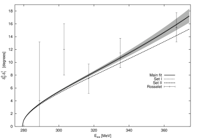
Figure 2: Phase shift difference $\delta_{0}^{0}-\delta_{1}^{1}$ to $O(p^{6})$ for different values of the $l_{i}^{r}(\mu)$ (Sets I, II [30]; main fit [22]) in comparison with experiment [31].

Preliminary new results from the $K_{e4}$ experiment in Brookhaven (BNL-E865 [32]) are in agreement with the theoretical predictions.

4.2 Dispersive matching

The most important development in recent years in the field of $\pi\pi$ scattering is the new dispersive analysis [33] via Roy equations [34] and the subsequent matching with the chiral amplitude [35] (that actually appeared after this meeting).

In a first step [33], the low partial waves ($S,P$) were derived from dispersion relations (Roy equations) with high-energy data ($E\geq 0.8$ GeV) as experimental input and with the scattering lengths $a_{0}^{0},a_{0}^{2}$ as subtraction constants. The output comes in the form of amazingly precise predictions for the phase shifts and for the remaining threshold parameters in terms of $a_{0}^{0},a_{0}^{2}$. However, even with the new results from BNL-E865 [32] included (the dash-dotted ellipse in Fig. 3), the allowed domain in the $a_{0}^{0}-a_{0}^{2}$ plane shown in Fig. 3 is still rather large although previously admissible values for $a_{0}^{0}$ of 0.26 or higher are practically ruled out now.

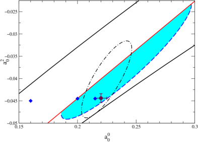
Figure 3: Various constraints on the scattering lengths $a_{0}^{0},a_{0}^{2}$ from Ref. [35]. The diamonds illustrate the convergence of the CHPT results of orders $p^{2},p^{4}$ and $p^{6}$. The cross shows the final result of Ref. [35] reproduced in (4.6).

In a second step, Colangelo, Gasser and Leutwyler [35] have matched the Roy-equation and $O(p^{6})$ solutions at the unphysical point $s=0$. The reason for this choice is that the chiral expansion converges better at $s=0$ than at the physical threshold $s=4M_{\pi}^{2}$. With the input of $l_{3}^{r},l_{4}^{r}$ (main sensitivity) and the $O(p^{6})$ LECs $r_{i}^{r}$ ($i=1,\dots,4$), this matching produces values for $l_{1}^{r},l_{2}^{r}$, $r_{5}^{r},r_{6}^{r}$ and especially for $a_{0}^{0},a_{0}^{2}$.

Some of the resulting threshold parameters are collected in the last column of Table 3. For comparison, the original predictions based on set I [30] of $O(p^{4})$ LECs and the predictions from the recent $O(p^{6})$ analysis [22] are also shown.

Table 3: Threshold parameters for $\pi\pi$ scattering

	$O(p^{6})$ main fit [22]	$O(p^{6})$ set I [30]	matching solution [33, 35]
$a^{0}_{0}$	$0.219\pm 0.005$	$0.222$	$0.220\pm 0.005$
$-10a^{2}_{0}$	$0.420\pm 0.010$	$0.420$	$0.444\pm 0.010$
$b^{0}_{0}$	$0.279\pm 0.011$	$0.282$	$0.276\pm 0.006$
$-10b^{2}_{0}$	$0.756\pm 0.021$	$0.729$	$0.803\pm 0.012$
$10a^{1}_{1}$	$0.378\pm 0.021$	$0.404$	$0.379\pm 0.005$
$10^{2}b^{1}_{1}$	$0.59\pm 0.12$	$0.83$	$0.567\pm 0.013$
$10^{2}a^{0}_{2}$	$0.22\pm 0.04$	$0.28$	$0.175\pm 0.003$
$10^{3}a^{2}_{2}$	$0.29\pm 0.10$	$0.24$	$0.170\pm 0.013$

The following conclusions emerge concerning our present understanding of $\pi\pi$ scattering in QCD.

i.

The chiral expansion “converges”. There are no signs of any unexpected large higher-order contributions.

ii.

The biggest contributions in many cases are well understood: they are due to chiral logs, especially for $S$-waves.

iii.

The state-of-the-art amplitude arising from the combination of CHPT to $O(p^{6})$ and dispersion theory (Roy equations) is in agreement with all available data. Additional forthcoming experimental results should put the theory to even more stringent tests.

iv.

Standard CHPT produces the following solid predictions for the $S$-wave scattering lengths [35] :

$$a_{0}^{0} = 0.220\pm 0.005$$

$$a_{0}^{2} = -0.0444\pm 0.0010~{}.$$ (4.6)

v.

These results depend on the standard values of $l_{3}^{r},l_{4}^{r}$ which Generalized CHPT may and does question. However, $a_{0}^{0}<0.25$ is a prediction from Roy equations only and therefore independent of the chiral expansion scheme.

vi.

A second caveat concerns the precision reached by the dispersive analysis. As stressed by the authors of Ref. [33], the errors in the last column of Table 3 should be interpreted as being due to the “experimental noise” seen in the analysis. At this level of accuracy, isospin violation and electromagnetic corrections must be included. The latter are partly available for $\pi\pi\to\pi\pi$ [36] but not (yet) for $K_{e4}$.

5 Isospin Violation

There are two sources of isospin violation in the standard model:

• $m_{u}\neq m_{d}$ (strong isospin violation);

• Electroweak interactions, in particular electromagnetic corrections.

The level of accuracy reached in many processes, experimentally and/or theoretically, calls for inclusion of the dominant isospin-violating effects. As an example, consider the dependence of the $\pi\pi$ scattering length $a_{0}^{0}$ on the pion mass in lowest order:

$$a_{0}^{0}=\frac{7M_{\pi}^{2}}{32\pi F_{\pi}^{2}}=\left\{\begin{array}[]{ll}0.159&\quad\qquad M_{\pi}=M_{\pi^{+}}\\ 0.149&\quad\qquad M_{\pi}=M_{\pi^{0}}\end{array}\right.~{}.$$ (5.1)

The difference is comparable to the corrections of $O(p^{6})$.

To locate the leading isospin-violating effects in $\pi\pi$ scattering, let us first look at the relevant part of the strong Lagrangian (for $N_{f}=2$ [2]):

$${\cal L}_{2}+{\cal L}_{4} = \frac{F^{2}}{4}\langle D_{\mu}UD^{\mu}U^{\dagger}+\chi U^{\dagger}+\chi^{\dagger}U\rangle$$ (5.2)

$$+ \dots-\frac{l_{7}}{16}\langle\chi U^{\dagger}-\chi^{\dagger}U\rangle^{2}~{}.$$

The term proportional to $l_{7}$ makes a tiny contribution to $M_{\pi^{0}}^{2}$ but there are no other consequences of $m_{u}\neq m_{d}$ for $\pi\pi\to\pi\pi$ to $O(p^{4})$. The leading effect is of electromagnetic origin due to the one-parameter Lagrangian ${\cal L}_{e^{2}p^{0}}^{\rm em}$ in Table 1:

$${\cal L}_{e^{2}p^{0}}^{\rm em}=e^{2}ZF^{4}\langle QUQU^{\dagger}\rangle$$ (5.3)

$$\to\qquad\Delta M_{\pi}^{2}=M_{\pi^{+}}^{2}-M_{\pi^{0}}^{2}=2e^{2}ZF^{2}~{},\quad Z\simeq 0.8~{}.$$ (5.4)

Again, there are no other contributions to $\pi\pi$ scattering in addition to the kinematical effect due to the mass shift (5.4). The genuine leading electromagnetic (and isospin-violating) corrections to the scattering amplitude are of $O(e^{2}p^{2})$.

5.1 Pionic atoms

The DIRAC experiment [37] at CERN attempts to measure the lifetime of electromagnetically bound $\pi^{+}-\pi^{-}$ “atoms” in the ground state to 10$\%$ accuracy. The width is dominated by the transition $\pi^{+}\pi^{-}\to\pi^{0}\pi^{0}$, with the $\pi^{0}$’s decaying subsequently into photons. Assuming isospin invariance for the amplitude, the decay width into two neutral pions is given by (LO stands for lowest order, i.e., without isospin violation) [38]

$$\Gamma_{2\pi^{0}}^{\rm LO}=\frac{2}{9}\alpha^{3}p^{*}(a_{0}^{0}-a_{0}^{2})^{2}~{}\to~{}\tau\simeq 3\times 10^{-15}s$$ (5.5)

where $p^{*}=(M_{\pi^{+}}^{2}-M_{\pi^{0}}^{2}-M_{\pi^{+}}^{2}\alpha^{2}/4)^{1/2}$ is the three-momentum of either $\pi^{0}$ in the final state (in the center of mass) and $a_{0}^{0}-a_{0}^{2}$ is the scattering length for $\pi^{+}\pi^{-}\to\pi^{0}\pi^{0}$. Therefore, DIRAC is expected to measure $|a_{0}^{0}-a_{0}^{2}|$ to 5$\%$ accuracy (cf. Fig. 3).

As already emphasized, this level of accuracy makes a careful estimate of isospin-violating corrections mandatory. Since in QCD $A(\pi\pi\to\pi\pi)$ does not contain terms linear in $m_{u}-m_{d}$ the leading corrections are $O(\delta)$ with $\delta=\alpha$ or $(m_{u}-m_{d})^{2}$ [39].

The effective field theory technique of Gall et al. [39] for calculating those corrections turns out to be superior to other previously or currently employed methods, like nonrelativistic potential or Bethe-Salpeter approaches. The method consists of the following main steps:

• The starting point is CHPT for $N_{f}=2$ with a dynamical photon.

• From CHPT, one passes to a nonrelativistic effective Lagrangian, similar to the procedure employed in QED [40]. To the order required, the electromagnetic interaction occurs only through the Coulomb potential [39].

• With this nonrelativistic Lagrangian, one calculates the energy of the bound state and the width $\Gamma_{2\pi^{0}}$ and matches the scattering amplitude to the full relativistic expression with $O(\delta)$ corrections included.

The final result [39] is a corrected rate

$$\Gamma_{2\pi^{0}}=\frac{2}{9}\alpha^{3}p^{*}A^{2}(1+K)$$ (5.6)

where $A$ is directly related to the relativistic on-shell scattering amplitude at threshold:

$$A=-\frac{3}{32\pi}\mbox{\rm Re}A_{\rm thr}(\pi^{+}\pi^{-}\to\pi^{0}\pi^{0})+o(\delta)~{}.$$ (5.7)

The quantity $K$ contains additional corrections :

$$K = \frac{\Delta M_{\pi}^{2}}{9M_{\pi}^{2}}(a_{0}^{0}+2a_{0}^{2})^{2}-\frac{2\alpha}{3}(\ln\alpha-1)(2a_{0}^{0}+a_{0}^{2})+o(\delta)$$ (5.8)

$$= 1.1\times 10^{-2}~{}.$$

The threshold amplitude $A$ is expanded to first order in $\delta$ :

$$A=a_{0}^{0}-a_{0}^{2}+h_{1}(m_{u}-m_{d})^{2}+h_{2}\alpha+o(\delta)~{}.$$ (5.9)

The scattering lengths $a_{0}^{0},a_{0}^{2}$ and the coefficients $h_{i}$ in this expansion are to be taken in the isospin limit for $M_{\pi}=M_{\pi^{+}}$. Since $h_{1}$ turns out to be negligible the uncertainty in the final result [41] is exclusively due to $h_{2}$ that depends both on the LECs $l_{i}^{r}$ (multiplied by the electromagnetic coupling constant $Z$ defined in Eq. (5.3)) and on LECs of $O(e^{2}p^{2})$ [42]:

$$A=a_{0}^{0}-a_{0}^{2}+\varepsilon~{},\qquad\varepsilon=(0.58\pm 0.16)\times 10^{-2}~{}.$$ (5.10)

Putting everything together, Gasser et al. [41] obtain for the relative isospin-violating correction

$$\frac{\Gamma_{2\pi^{0}}-\Gamma_{2\pi^{0}}^{\rm LO}}{\Gamma_{2\pi^{0}}^{\rm LO}}=\underbrace{\displaystyle\frac{2\varepsilon}{a_{0}^{0}-a_{0}^{2}}}_{0.047}+\underbrace{K}_{0.011}=0.058~{}.$$ (5.11)

Since the experimental accuracy for $\Gamma_{2\pi^{0}}$ is expected to be 10$\%$ the above 6$\%$ correction due to isospin violation is crucial for extracting $|a_{0}^{0}-a_{0}^{2}|$ from experiment. This combination can then be directly compared to the CHPT calculation for $\alpha=0,m_{u}=m_{d}$, as discussed in Sec. 4.

5.2 CP violation and $\pi^{0}-\eta$ mixing

Isospin violation is usually a small effect. Unlike for $\pi\pi$ scattering where terms linear in $m_{u}-m_{d}$ are absent, the following order-of-magnitude estimates should be relevant for $N_{f}=3$, in particular for $K$ decays:

$O(m_{u}-m_{d})$	$O(\alpha)$
$\displaystyle\frac{M_{K^{0}}^{2}-M_{K^{+}}^{2}}{M_{K}^{2}}\sim 1.5\%$	$\displaystyle\frac{M_{\pi^{+}}^{2}-M_{\pi^{0}}^{2}}{M_{K}^{2}}\sim 0.5\%$

In general, strong isospin violation and electromagnetic corrections are comparable in size and the effect is quite small unless there is some specific enhancement mechanism. This is precisely the case for the dominant decays of kaons into two pions. Restricting the discussion to $K^{0}$ decays, the amplitudes in the isospin limit are usually parametrized as [6]

$$A(K^{0}\to\pi^{+}\pi^{-}) = A_{0}e^{i\delta^{0}_{0}}+\frac{1}{\sqrt{2}}A_{2}e^{i\delta^{2}_{0}}$$

$$A(K^{0}\to\pi^{0}\pi^{0}) = A_{0}e^{i\delta^{0}_{0}}-\sqrt{2}A_{2}e^{i\delta^{2}_{0}}$$ (5.12)

with $\delta_{l=0}^{I}$ the $\pi\pi$ phase shifts at $s=M_{K}^{2}$. Although the amplitudes $A_{0},A_{2}$ could well be similar in size (in fact, they are in the so-called “naive” factorization limit) they are actually quite different in the real world as expressed by the $\Delta I=1/2$ “rule”:

$$A_{2}/A_{0}\simeq 1/22~{}.$$ (5.13)

This rule suggests a possible strong enhancement of isospin-violating corrections in $A_{2}$, e.g.,

$$A_{2}^{\rm ind}/A_{2}\sim\frac{M_{K^{0}}^{2}-M_{K^{+}}^{2}}{M_{K}^{2}}\cdot\frac{A_{0}}{A_{2}}\simeq 0.35~{}.$$ (5.14)

One instance where this enhancement can be seen is the CP violating ratio $\varepsilon^{\prime}/\varepsilon$. In the approximate formula [43]

$$\frac{\varepsilon^{\prime}}{\varepsilon}\approx 13\,\mbox{\rm Im}V_{ts}^{*}V_{td}\left[B_{6}^{(1/2)}(1-\Omega_{IB})-0.4B_{8}^{(3/2)}\right]$$ (5.15)

the quantity

$$\Omega_{IB}:=\frac{\mbox{\rm Im}A_{2}^{\rm IB}\mbox{\rm Re}A_{0}}{\mbox{\rm Im}A_{0}\mbox{\rm Re}A_{2}}$$ (5.16)

is a measure of strong isospin violation. The so-called bag factors [6] $B_{6}^{(1/2)},B_{8}^{(3/2)}$ are parameters of $O(1)$ and $V_{ij}$ are Cabibbo-Kobayashi-Maskawa matrix elements.

To lowest order in the chiral expansion, $\Omega_{IB}$ is due to $\pi^{0}-\eta$ mixing:

$$\Omega_{IB} = \frac{2\sqrt{2}\varepsilon_{\pi^{0}\eta}^{(2)}}{3\sqrt{3}\omega}=0.13$$ (5.17)

$$\varepsilon_{\pi^{0}\eta}^{(2)} = \frac{\sqrt{3}(m_{d}-m_{u})}{4(m_{s}-\hat{m})}~{}.$$ (5.18)

At $O(p^{4})=O[(m_{u}-m_{d})p^{2}]$, there is a large contribution from $\eta^{\prime}$ exchange [44]:

$$\Omega_{\eta+\eta^{\prime}}=0.25\pm 0.08~{}.$$ (5.19)

Such a big correction raises the legitimate question whether there are other contributions to $\Omega_{IB}$ at the same order. One part of the problem is related to the higher-order corrections to the $\pi^{0}-\eta$ mixing angle. Writing

$$\varepsilon_{\pi^{0}\eta}=\varepsilon_{\pi^{0}\eta}^{(2)}+\varepsilon_{\pi^{0}\eta}^{(4)}~{},$$

one finds [45, 46]

$$\varepsilon_{\pi^{0}\eta}^{(4)}/\varepsilon_{\pi^{0}\eta}^{(2)} = \frac{128(M^{2}_{K}-M^{2}_{\pi})^{2}}{3F_{\pi}^{2}(M_{\pi}^{2}-M_{\eta}^{2})}\left[3L_{7}+L^{r}_{8}(M_{\rho})\right]$$ (5.20)

$$+ {\rm~{}(small)~{}~{}loop~{}~{}corrections}~{}.$$

Of the three contributions in (5.20), the first one contains the previously mentioned $\eta^{\prime}$ exchange:

$$\varepsilon_{\pi^{0}\eta}^{(4)}(L_{7})/\varepsilon_{\pi^{0}\eta}^{(2)}=1.10~{},$$ (5.21)

perfectly consistent with the old estimate (5.19). The surprise comes from the second term that was not included previously and in fact almost cancels the $L_{7}$ term [46]:

$$\varepsilon_{\pi^{0}\eta}^{(4)}(L_{8}^{r}(M_{\rho}))/\varepsilon_{\pi^{0}\eta}^{(2)}=-0.83~{}.$$ (5.22)

One reason why this part was not included originally is the physical interpretation of the LEC $L_{8}$: it is dominated by $a_{0}(980)$ exchange and its relevance for $\Omega_{IB}$ is much less transparent than $\eta^{\prime}$ exchange. The loop corrections in (5.20) are negligible for $\mu=M_{\rho}$.

The total contribution from $\pi^{0}-\eta$ mixing to $\Omega_{IB}$ with

$$3L_{7}+L_{8}^{r}(M_{\rho})=(-0.25\pm 0.25)\cdot 10^{-3}$$

amounts to

$$\Omega_{IB}^{\pi^{0}\eta}=0.16\pm 0.03~{}.$$ (5.23)

With the preferred bag factors of the Munich group [43], a decrease from $\Omega_{IB}=0.25$ to 0.16 implies an increase of $\varepsilon^{\prime}/\varepsilon$ by 21$\%$.

The systematic analysis of isospin-violating corrections at next-to-leading order also shows that there are additional contributions proportional to $m_{u}-m_{d}$ that depend on largely unknown weak LECs. Model-dependent estimates suggest [47] an additional decrease of $\Omega_{IB}$ below (5.23).

6 Outlook

Chiral perturbation theory is the effective field theory of the standard model at low energies. It is a nonrenormalizable but perfectly well-defined and respectable quantum field theory. One of its major advantages is the absence of double counting: in contrast to many phenomenological models, only hadronic fields enter in the chiral Lagrangians. The price for the generality of CHPT is the abundance of low-energy constants at higher orders in the chiral expansion.

CHPT has undoubtedly reached a level of maturity. In the meson sector, two-loop calculations are state of the art for the strong interactions and there is little to gain from going even further. The main task in this area for the near future is the evaluation of “small” effects due to isospin violation and electromagnetic corrections. There is more work to be done for the nonleptonic weak interactions [6].

For single-baryon processes, even the complete one-loop amplitudes remain to be calculated for some transitions. The slow convergence of the chiral expansion may require a reordering of the series. Chiral symmetry in nuclear physics is still a rapidly expanding field.

Even a superficial look at the effective Lagrangian of the standard model in Table 1 tells us that phenomenology cannot possibly fix all the low-energy constants of this Lagrangian. Progress in the field will depend to a large degree on the success of supplementary methods to determine those parameters.

References

- [1] S. Weinberg, Physica 96A (1979) 327.
- [2] J. Gasser and H. Leutwyler, Ann. Phys. 158 (1984) 142.
- [3] J. Gasser and H. Leutwyler, Nucl. Phys. B250 (1985) 465.
- [4] H. Leutwyler, Ann. Phys. 235 (1994) 165.
- [5] M. Knecht, S. Peris and E. de Rafael, Nucl. Phys. Proc. Suppl. 86 (2000) 279.
- [6] J. Bijnens, Weak interactions of light flavours, in these Proceedings.
- [7] J. Heitger, R. Sommer and H. Wittig, hep-lat/0006026.
- [8] R. Kaiser and H. Leutwyler, hep-ph/0007101, to appear in Eur. Phys. J. C.
- [9] G. Ecker, Chiral symmetry, Proc. of 37. Internationale Universitätswochen für Kern– und Teilchenphysik, Schladming, Feb. 1998, Eds. L. Mathelitsch and W. Plessas, Lecture Notes in Physics, Vol. 521, Springer (Heidelberg, 1999), hep-ph/9805500.
- [10] J. Goldstone, Nuovo Cim. 19 (1961) 154.
- [11] B. Moussallam, Eur. Phys. J. C14 (2000) 111; JHEP 0008 (2000) 005.
- [12] S. Descotes, L. Girlanda and J. Stern, JHEP 0001 (2000) 041.
- [13] J. Stern, Light quark masses and condensates in QCD, in Ref. [19].
- [14] S. Weinberg, Phys. Rev. Lett. 17 (1966) 616.
-
[15]
G. Ecker, J. Gasser, A. Pich and E. de Rafael, Nucl. Phys. B321 (1989)
311 ;
G. Ecker, J. Gasser, H. Leutwyler, A. Pich and E. de Rafael, Phys. Lett. B223 (1989) 425. - [16] E. Jenkins and A.V. Manohar, Phys. Lett. B255 (1991) 558.
- [17] T. Becher and H. Leutwyler, Eur. Phys. J. C9 (1999) 643.
- [18] S.R. Beane et al., nucl-th/0008064.
- [19] A.M. Bernstein, D. Drechsel and T. Walcher, Proc. of Chiral Dynamics: Theory and Experiment, Mainz, Germany, Sept. 1997, Lecture Notes in Physics, Vol. 513, Springer (Heidelberg, 1998).
- [20] J. Bijnens and U.-G. Meißner, Chiral Effective Theories, Mini-Proceedings of the Workshop on Chiral Effective Theories, Bad Honnef, Germany, Dec. 1998, hep-ph/9901381.
- [21] Chiral Dynamics 2000: Theory and Experiment, Jefferson Lab., Newport News, VA, USA, July 2000, http://www.jlab.org/intralab/calendar/chiral.html.
- [22] G. Amoros, J. Bijnens and P. Talavera, Phys. Lett. B480 (2000) 71; Nucl. Phys. B585 (2000) 293.
- [23] J. Bijnens, G. Colangelo and G. Ecker, Annals of Phys. 280 (2000) 100.
- [24] J. Bijnens, G. Colangelo and G. Ecker, JHEP 02 (1999) 020.
- [25] J. Bijnens, G. Colangelo and G. Ecker, Phys. Lett. B441 (1998) 437.
- [26] J. Stern, H. Sazdjian and N.H. Fuchs, Phys. Rev. D47 (1993) 3814.
- [27] J. Gasser and H. Leutwyler, Phys. Lett. 125B (1983) 325.
- [28] M. Knecht, B. Moussallam, J. Stern and N.H. Fuchs, Nucl. Phys. B457 (1995) 513.
- [29] M. Knecht, B. Moussallam, J. Stern and N.H. Fuchs, Nucl. Phys. B471 (1996) 445.
- [30] J. Bijnens, G. Colangelo, G. Ecker, J. Gasser and M.E. Sainio, Phys. Lett. B374 (1996) 210; Nucl. Phys. B508 (1997) 263.
- [31] L. Rosselet et al., Phys. Rev. D15 (1977) 574.
- [32] M.E. Zeller (BNL-E865), Measurement of the properties of the decay , Talk given at Chiral Dynamics 2000 [21].
- [33] B. Ananthanarayan, G. Colangelo, J. Gasser and H. Leutwyler, hep-ph/0005297.
- [34] S.M. Roy, Phys. Lett. B36 (1971) 353.
- [35] G. Colangelo, J. Gasser and H. Leutwyler, Phys. Lett. B488 (2000) 261.
-
[36]
M. Knecht and R. Urech, Nucl. Phys. B519 (1998) 329;
U.-G. Meißner, G. Müller and S. Steininger, Phys. Lett. B406 (1997) 154; Err, ibid. B407 (1997) 454. - [37] M. Pentia (DIRAC-Collaboation), hep-ph/0001279 and references therein.
- [38] S. Deser, M.L. Goldberger, K. Baumann and W. Thirring, Phys. Rev. 96 (1954) 774.
- [39] A. Gall, J. Gasser, V.E. Lyubovitskij and A. Rusetsky, Phys. Lett. B462 (1999) 335.
- [40] W.E. Caswell and G.P. Lepage, Phys. Lett. B167 (1986) 437.
- [41] J. Gasser, V.E. Lyubovitskij and A. Rusetsky, Phys. Lett. B471 (1999) 244.
- [42] R. Urech, Nucl. Phys. B433 (1995) 234.
- [43] S. Bosch et al., Nucl. Phys. B 565 (2000) 3.
-
[44]
J.F. Donoghue, E. Golowich, B.R. Holstein and J. Trampetic,
Phys. Lett. B179 (1986) 361;
A.J. Buras and J.-M. Gérard, Phys. Lett. B192 (1987) 156;
H.-Y. Cheng, Phys. Lett. B201 (1988) 155;
M. Lusignoli, Nucl. Phys. B325 (1989) 33. - [45] J. Gasser and H. Leutwyler, Nucl. Phys. B250 (1985) 517.
- [46] G. Ecker, G. Müller, H. Neufeld and A. Pich, Phys. Lett. B477 (2000) 88.
-
[47]
S. Gardner and G. Valencia, Phys. Lett. B466 (1999) 355;
C.E. Wolfe and K. Maltman, Phys. Lett. B482 (2000) 77; hep-ph/0007319.