RECENT DEVELOPMENTS IN CHIRAL PERTURBATION THEORY

Abstract

I briefly review the current status of chiral perturbation theory (CHPT) in the meson sector. Emphasis is given on the quest for higher precision. I discuss two examples: one where it is difficult to make a good prediction ($K_{L}\to\pi^{0}\gamma\gamma$), and where CHPT, even when pushed to higher orders, cannot yield an increase in accuracy. The second one is $\pi\pi$ scattering where a very sharp prediction can be made by combining CHPT at the two–loop level with dispersion relations.

1 Introduction

Chiral perturbation theory (CHPT) is the low–energy effective theory of the strong interactions. It yields a systematic expansion of any Green function in powers of quark masses and momenta, that automatically respects the Ward identities implied by the chiral symmetry of the strong interactions. Its present form is due to Weinberg [1] and Gasser and Leutwyler [2]. They showed the advantages of the effective–field–theory language over the direct implementation of the Ward identities as in the current–algebra framework. In particular, what was known before as a very difficult problem, the calculation of the unitarity corrections to a current–algebra result, was reduced to a routine loop calculation in a well–defined framework. After the convenient tools of the effective field theory were made available, many processes have been calculated at the one–loop level: wherever possible, the comparison to the experimental data has shown a remarkable success of the method.

In the early nineties several precision experiments on kaons, pions and etas, were approved, and brought the challenge of increasing the precision in CHPT calculations. Going beyond one loop became a necessity. The first complete two–loop calculation concerned the cross section for the two–photon annihilation into two neutral pions [3]. This beautiful and difficult calculation opened up the field of two–loop calculations in CHPT, that was very active during the nineties. In fact if we consider only the two–light–flavour sector, all the phenomenologically relevant calculations have already been completed, whereas in the $SU(3)$ framework, they have started only in more recent years [4, 5]. Moreover, in the purely strong sector, the Lagrangian at order $p^{6}$ and the complete divergence structure have been recently calculated [6].

In an effective theory it is not obvious that a higher loop calculation may lead to higher precision: new constants come into play at each order, and since they are a priori unknown, they may induce an uncertainty which is as large as the effect that one is calculating. The quest for higher precision within an effective field theory is a particularly nontrivial one. In what follows I will discuss in some detail why it is nontrivial, and how, in some special cases, one can nevertheless succeed in making very accurate predictions.

2 The Lagrangian of chiral perturbation theory

At lowest order the Lagrangian of CHPT is remarkably simple:

$${\cal L}^{(2)} = {F^{2}\over 4}\langle D_{\mu}UD^{\mu}U^{\dagger}+U\chi^{\dagger}+\chi U^{\dagger}\rangle+C\langle QUQU^{\dagger}\rangle$$ (1)

$$+ c_{2}\langle\lambda_{6}D_{\mu}U^{\dagger}D^{\mu}U\rangle+c_{3}{(27_{L},1_{R})}\;\;,$$

where

$$D_{\mu}U = \partial_{\mu}U-ir_{\mu}U+iUl_{\mu}\;\;\;\;\chi=2B(M+s+ip)$$

$$M = \mbox{diag}(m_{u},m_{d},m_{s})\;\;\;\ Q=e\cdot\mbox{diag}(2/3,-1/3,-1/3)\;\;,$$ (2)

where $U$ is the usual exponential of the matrix containing the octet of the Goldstone bosons, while $r_{\mu},\;l_{\mu},\;s$ and $p$ are matrices of external fields. $\langle A\rangle$ stands for the trace of $A$. The simplicity of this Lagrangian is particularly remarkable in view of the variety of phenomena that it describes: the first two terms describe the strong interactions of the octet of the pseudoscalars between themselves and with external sources. The third, proportional to $C$ describes the electromagnetic effects due to the exchanges of one virtual photon, while the remaining terms account for the effects generated by virtual exchanges of a $W$ or a $Z$ between quarks.

The five constants which appear in the Lagrangian are not fixed by the symmetry but are easily determined in the comparison to the simplest of the observables:

$$F_{\pi} = F+O(m)\;\;,\;\;\;\;M_{\pi^{0}}^{2}=B(m_{u}+m_{d})\;\;,$$

$$M_{\pi^{+}}^{2}-M_{\pi^{0}}^{2} = 2e^{2}{C\over F^{2}}\;\;,\;\;\;A^{(1/2)}_{K\to\pi\pi}\sim c_{2}-{2\over 3}c_{3}\;,\;\;A^{(3/2)}_{K\to\pi\pi}\sim c_{3}\;.$$ (3)

Having fixed these constants, we can now calculate any other new observable, and make a prediction. For example the $\pi\pi$ scattering amplitude and the $K_{l3}$ form factors are given by:

$$A(s,t,u)={s-M_{\pi}^{2}\over F_{\pi}^{2}}\Rightarrow a_{0}^{0}={7M_{\pi}^{2}\over 32\pi F_{\pi}^{2}}=0.16\;,$$ (4)

$$\langle\pi^{-}(p)|V_{\mu}|K^{0}(k)\rangle = (k+p)_{\mu}f_{+}(t)+(k-p)_{\mu}f_{-}(t)\;\;,\;\;\;t=(k-p)^{2}\;\;$$

$$f_{+}(t) = 1\;\;,\;\;\;f_{-}(t)=0\;\;.$$ (5)

2.1 The Lagrangian at next–to–leading order and beyond: strong sector

In the strong sector the situation is the following:

$$O(p^{2}) \Rightarrow {F^{2}\over 4}\langle D_{\mu}UD^{\mu}U^{\dagger}+U\chi^{\dagger}+\chi U^{\dagger}\rangle\;\;,$$

$$O(p^{4}) \Rightarrow \mbox{10 new LEC, Gasser and Leutwyler \cite[cite]{[\@@bibref{}{GL}{}{}]} (84)},\;\;L_{i}\;\;,$$

$$O(p^{6}) \Rightarrow \mbox{96 new LEC, Bijnens, G.C., Ecker \cite[cite]{[\@@bibref{}{lagrp6}{}{}]} (99)},\;\;C_{i}\;\;.$$

For all the ten $L_{i}$’s we have either a good phenomenological determination, or a sound theoretical estimate. In order to get a prediction at order $p^{4}$ in this sector one simply needs to do the one–loop calculation, remove the divergences with the help of the counterterms, and insert the numerical values of the finite parts from the most recent estimates. At this level the situation is almost as good as at order $p^{2}$. This is best seen with a couple of examples, like the $\pi\pi$ scattering lengths and the $K_{e3}$ form factors, that we have seen before at leading order. The next–to–leading order corrections are [2, 7]

$$a_{0}^{0}\! = \!{7M_{\pi}^{2}\over 32\pi F_{\pi}^{2}}\left[1+{M_{\pi}^{2}\over 3}\langle r^{2}\rangle_{S}^{\pi}+{200\pi F_{\pi}^{2}M_{\pi}^{2}\over 7}(a_{2}^{0}+2a_{2}^{2})+{M_{\pi}^{2}\over 16\pi^{2}F_{\pi}^{2}}\Delta_{0}^{0}\right]$$ (6)

$$= 0.16\cdot\left[1.25\right]=0.20\;\;,$$

$$f_{+}(t) = f_{+}(0)\left(1+\lambda_{+}{t\over M_{\pi}^{2}}\right)\;,\;\lambda_{+}={M_{\pi}^{2}\over 6}\langle r\rangle^{\pi}_{V}+\Delta_{+}=0.031\;\;.$$ (7)

The formulae above neatly illustrate the beauty of the method: the $S$–wave scattering lengths and the $K_{e3}$ form factors are expressible in terms of other observables (like the scalar and vector radii, $\langle r^{2}\rangle_{S}^{\pi}$ and $\langle r\rangle^{\pi}_{V}$, respectively, the two $D$–wave scattering lengths, $a_{2}^{0,2}$), plus other small corrections (indicated by the $\Delta$ symbols). The relation between these observables is exact up to order $p^{4}$, and will get corrections if we want to increase the precision of the calculation. By inserting the most recent values for the observables on the right–hand sides, one gets the numerical predictions given above. We will discuss the situation for the $\pi\pi$ scattering lengths in detail below. As for the $K_{e3}$ form factors, the slope $\lambda_{+}$ is quite well known, and the PDG [8] reports a number which is in excellent agreement with the one loop calculation above: $\lambda_{+}=0.0286\pm 0.0022$.

If we move up to order $p^{6}$ the situation worsens considerably, and it becomes impossible to write down expressions as nice as those in Eq. (67). We have to give expressions in terms of the new low–energy constants $C_{i}$’s, and since we know practically nothing about them, it is an obvious question whether these calculations represent an improvement at all in the final numerical predictions. Before discussing the matter in more detail in the following sections, we can already anticipate an answer at the intuitive level: The low–energy constants parametrise our ignorance of the dynamics which is not explicitly present in the formalism. They contain contributions from all the physics above the scale of the pseudoscalar mesons – the most prominent effect is the one due to the lowest–lying resonances, as it has been explicitly shown [9] at order $p^{4}$. Whenever a resonance or any other “high–energy” phenomenon is expected to influence substantially a low–energy quantity, one should expect a very important role of the low–energy constants, and a serious difficulty in making a precise prediction. On the other hand, observables dominated by the dynamics of the pseudoscalar, can be very well calculated within CHPT, and it makes good sense to push the calculations to order $p^{6}$, as one can expect the contribution of the low–energy constants to be suppressed. Explicit examples of both situations are given below.

2.2 The Lagrangian at next–to–leading order and beyond: weak and electromagnetic sectors

Both in the electromagnetic and weak sector, the situation becomes unpleasant already at next–to–leading order, where the number of constants immediately gets too large in comparison to the available experimental input:

E.m. sector:

$$O(p^{2}) \Rightarrow C\langle QUQU^{\dagger}\rangle\;\;,$$

$$O(p^{4}) \Rightarrow \mbox{21 new LEC, Urech, Neufeld and Rupertsberger \cite[cite]{[\@@bibref{}{urech}{}{}]} (93)},\;\;K_{i}\;\;,$$

Weak sector:

$$O(p^{2}) \Rightarrow c_{2}\langle\lambda_{6}D_{\mu}U^{\dagger}D^{\mu}U\rangle$$

$$O(p^{4}) \Rightarrow \mbox{37 new LEC, Kambor, Missimer, Wyler, Ecker \cite[cite]{[\@@bibref{}{weak_lagr}{}{}]} (91)},\;\;N_{i}\;\;.$$

In both cases, given the practical unfeasibility of a determination of all the available constants, the typical strategy has been to focus on a few selected processes where the same constants occur. One can then exploit the experimental information on some processes to make predictions in other. There are plenty of examples in the literature. A fairly comprehensive review of the situation in the weak sector (especially for the radiative decays), including a list of the new experimental measurements that are possible at a $\Phi$ factory can be found in Ref. [12].

3 Analysis of $K\to\pi\gamma\gamma$ up to order $p^{6}$.

Assuming $CP$ conservation the $A(K_{L}\to\pi^{0}\gamma\gamma)$ is determined by two invariant amplitudes, $A(s,\nu)$ and $B(s,\nu)$, $s=(q_{1}+q_{2})^{2},\nu=p_{K}\cdot(q_{1}-q_{2})$, where $q_{1,2}$ are the momenta of the two photons, and $p_{K}$ that of the kaon. At order $p^{2}$: $A=B=0$. At order $p^{4}$ [13]: $A=4/s(s-M_{\pi}^{2})F(s/M_{\pi}^{2})+\ldots$, and $B=0$, where $F(x)$ is a loop function generated by the $\pi\pi$ intermediate state in the $s$ channel, that represents the dominant effect at this order, and the ellipsis stands for other less important contributions. Although the shape of the spectrum was nicely confirmed by the experiment [14, 15], the branching ratio was a factor three too small:

$$BR=\left\{\begin{array}[]{lr}(1.7\pm 0.3)\times 10^{-6}&(\mbox{NA31})\\ (1.86\pm 0.60\pm 0.60)\times 10^{-6}&(\mbox{E731})\\ 0.67\times 10^{-6}&~{}~{}~{}~{}~{}~{}O(p^{4})\;\;,\end{array}\right.$$ (8)

therefore requiring large $O(p^{6})$ corrections. The calculations at order $p^{6}$ [16] have considered only the (possibly dominant) corrections to the pion loops, and added to this a polynomial contribution:

$$A = {4\over s}(s-M_{\pi}^{2})\tilde{F}\left({s\over M_{\pi}^{2}}\right)+4a_{V}\frac{3M_{K}^{2}-s-M_{\pi}^{2}}{M_{K}^{2}}+\ldots$$

$$B = \tilde{G}\left({s\over M_{\pi}^{2}}\right)-8a_{V}+\ldots\;\;,$$

where $\tilde{F}(x)$ and $\tilde{G}(x)$ also come from the $\pi\pi$ intermediate state in the $s$ channel. To get into agreement with the experiment one needed to have a large and negative $a_{V}$: $BR=0.83\times 10^{-6}$ with $a_{V}=0$ and $BR=1.60\times 10^{-6}$ with $a_{V}=-0.9$. Also for the spectrum, unitarity corrections alone were not sufficient (and actually worsened the comparison), while an improved agreement with the data is obtained only with $a_{V}\sim-0.9$.

The outcome of this $O(p^{6})$ analysis is therefore a clear need for a very large contribution from the polynomial part. Do we have a dynamical explanation for such a large constant? I find it instructive to go back by seven years and see how the situation appeared then: Cohen, Ecker and Pich in Ref. [13] described the situation as follows: “Several model estimates of $a_{V}$ have been made in the literature. A fair summary of those attempt is that we know neither the sign nor the magnitude of $a_{V}$.” More recently, however, D’Ambrosio and Portolés [17] have built a Vector Resonance Model that does indeed get the right sign and size for this constant: $a_{V}^{DP}\simeq-0.72$. This number is now in amazing agreement with the one extracted from a fit to the most recent data [18].

Although D’Ambrosio and Portolés estimate of $a_{V}$ was only a postdiction, it is reassuring to have an understanding of the size of this constant. In fact it is not the only case where one can find this relative size between the various contributions in the chiral expansion. A well–known analogous example in the strong sector is the vector form factor. Its Taylor expansion around $s=0$ is usually defined as $F_{V}(s)=1+1/6\langle r^{2}\rangle^{\pi}_{V}s+c_{V}^{\pi}s^{2}+O(s^{3})$. $c_{V}^{\pi}$ vanishes at order $p^{2}$, and can be predicted with no parameters at order $p^{4}$. Nowadays it is known up to order $p^{6}$ [19]:

$$c_{V}^{\pi} = \frac{1}{960\pi^{2}M_{\pi}^{2}F_{\pi}^{2}}+\frac{1}{(16\pi^{2}F_{\pi}^{2})^{2}}\left[\mbox{``}\ln{M_{\pi}^{2}\over\mu^{2}}\mbox{''}+\mbox{``}l_{i}^{r}\mbox{''}\right]+\frac{r^{r}_{V2}}{F_{\pi}^{4}}$$

$$= (0.62+1.96+1.3\cdot 10^{-4}r^{r}_{V2}(M_{\rho}))\,{\rm GeV}^{-4}=5.4\,{\rm GeV}^{-4}\;,$$

where the latter value is determined experimentally. Here also: i) the order $p^{4}$ parameter–free prediction fails badly; ii) there are large $O(p^{6})$ unitarity corrections; iii) but even larger $O(p^{6})$ polynomial contributions, coming from the well–known $\rho$ resonance.

4 $\pi\pi$ scattering at order $p^{6}$

This is the “golden reaction” for Chiral Perturbation Theory: at threshold the naive expansion parameter is $M_{\pi}^{2}/1\,{\rm GeV}^{2}\sim 0.02$, and already a tree level calculation [20] should be rather accurate, in principle. However, this rule of thumb is quite misleading here, as it is shown by the fact that both the one–loop [21] (see Eq. (6)) and the two–loop [22] calculations produced substantial corrections. The violation of the rule of thumb has a well known origin, and is due to the presence of chiral logarithms $L=M_{\pi}^{2}/(4\pi F_{\pi})^{2}\ln M^{2}/\mu^{2}$, which, for $\mu\sim 1$ GeV change the expansion parameter by a factor four. If we look at the $I=0$ $S$–wave scattering lengths, e.g., a large coefficient in front of the single (at one loop) and double (at two loops) chiral logarithms is the main source of the large correction [21, 23]:

$$a^{0}_{0}=\frac{7M_{\pi}^{2}}{32\pi F_{\pi}^{2}}\left\{1-\frac{9}{2}L+\frac{857}{42}L^{2}+\ldots\right\}=0.217$$ (10)

The final number is the estimate given by the authors of the complete two–loop calculation [22], and was given without an estimate of the uncertainties, that required considerably more work. A better numerical prediction with an accurate estimate of the uncertainties is now available [24], but before describing how this was obtained, it is useful to analyse in more detail the number in Eq. (10).

In particular it is important to check the role of the new (and largely unknown) $O(p^{6})$ constants. In this case their influence is rather small: to obtain the number in Eq. (10) they were estimated using resonance saturation [22]. However, if one puts them to zero, the change in $a_{0}^{0}$ is less than 1%. For the analytic part of the chiral expansion the rule of thumb works quite well. On the other hand it is more worrisome the effect of the uncertainties in the $O(p^{4})$ constants, supposedly known quite well: changing the constants within their error bars changes the value of $a_{0}^{0}$ typically by 0.01: The two–loop contribution can be completely overshadowed by the uncertainty coming from the $O(p^{4})$ constants – to improve the prediction one has to reduce drastically this uncertainty. This improvement in precision has been obtained by the use of a different method to determine the low–energy constants which we are now going to describe.

4.1 Dispersive representation of the scattering amplitude

As shown by Roy [25], the fixed-$t$ dispersion relations can be written in such a form that they express the $\pi\pi$ scattering amplitude in terms of the imaginary parts in the physical region of the $s$-channel. The resulting representation for $A(s,t,u)$ contains two subtraction constants, which may be identified with the scattering lengths $a^{0}_{0}$ and $a^{2}_{0}$. Unitarity converts this representation into a set of coupled integral equations, which was recently examined in detail [26]. The upshot of that analysis is that $a_{0}^{0}$ and $a_{0}^{2}$ are the essential low energy parameters: Once these are known, the available experimental data determine the behaviour of the $\pi\pi$ scattering amplitude at low energies to within remarkably small uncertainties.

The branch cut generated by the imaginary parts of the partial waves with $\ell\geq 2$ starts manifesting itself only at $O(p^{8})$. Accordingly, we may expand the corresponding contributions to the dispersion integrals into a Taylor series of the momenta. The singularities due to the imaginary parts of the $S$- and $P$-waves, on the other hand, show up already at $O(p^{4})$ – these cannot be replaced by a polynomial. We subtract the corresponding dispersion integrals as many times as is needed in the chiral representation, for later convenience:

$$\,\overline{\rule[7.5pt]{8.99994pt}{0.0pt}}W^{I}(s) \!\!= \!\!\frac{s^{4-\epsilon_{I}}}{\pi}\int_{4M_{\pi}^{2}}^{\infty}ds^{\prime}\;\frac{\mbox{Im}\,t^{I}(s^{\prime})}{s^{\prime\,4-\epsilon_{I}}(s-4M_{\pi}^{2})^{\epsilon_{I}}(s^{\prime}-s)}\;\;,$$ (11)

where $\{\epsilon_{0},\epsilon_{1},\epsilon_{2}\}=\{0,1,0\}$. Since all other contributions can be replaced by a polynomial, the phenomenological amplitude takes the form

$$A(s,t,u) \!\!= \!\!16\pi a_{0}^{2}+\frac{4\pi}{3M_{\pi}^{2}}\,(2a_{0}^{0}-5a_{0}^{2})\,s+\,\overline{\rule[7.5pt]{5.0pt}{0.0pt}}P(s,t,u)+32\pi\left\{\mbox{$\frac{1}{3}$}\,\overline{\rule[7.5pt]{8.99994pt}{0.0pt}}W^{0}(s)-\mbox{$\frac{1}{3}$}\,\overline{\rule[7.5pt]{8.99994pt}{0.0pt}}W^{2}(s)\right.$$

$$\!\!+ \!\!\left.\mbox{$\frac{3}{2}$}(s-u)\,\overline{\rule[7.5pt]{8.99994pt}{0.0pt}}W^{1}(t)+\mbox{$\frac{3}{2}$}(s-t)\,\overline{\rule[7.5pt]{8.99994pt}{0.0pt}}W^{1}(u)+\mbox{$\frac{1}{2}$}\,\overline{\rule[7.5pt]{8.99994pt}{0.0pt}}W^{2}(t)+\mbox{$\frac{1}{2}$}\,\overline{\rule[7.5pt]{8.99994pt}{0.0pt}}W^{2}(u)\right\}+O(p^{8})\,.$$

We have explicitly displayed the contributions from the subtraction constants $a_{0}^{0}$ and $a_{0}^{2}$. The term $\,\overline{\rule[7.5pt]{5.0pt}{0.0pt}}P(s,t,u)$ is a crossing symmetric polynomial

$$\,\overline{\rule[7.5pt]{5.0pt}{0.0pt}}P(s,t,u) \!\!= \!\!\overline{\rule[5.0pt]{3.99994pt}{0.0pt}}p_{1}+\overline{\rule[5.0pt]{3.99994pt}{0.0pt}}p_{2}\,s+\overline{\rule[5.0pt]{3.99994pt}{0.0pt}}p_{3}\,s^{2}+\overline{\rule[5.0pt]{3.99994pt}{0.0pt}}p_{4}\,(t-u)^{2}+\overline{\rule[5.0pt]{3.99994pt}{0.0pt}}p_{5}\,s^{3}+\overline{\rule[5.0pt]{3.99994pt}{0.0pt}}p_{6}\,s(t-u)^{2}\;\;.$$ (12)

Its coefficients can be expressed in terms of integrals over the imaginary parts of the partial waves. In the following, the essential point is that the coefficients $\overline{\rule[5.0pt]{3.99994pt}{0.0pt}}p_{1},\ldots\,,\,\overline{\rule[5.0pt]{3.99994pt}{0.0pt}}p_{6}$ can be determined phenomenologically [26].

In the chiral representation we have, similarly

$$A(s,t,u) \!\!= \!\!C(s,t,u)+32\pi\left\{\mbox{$\frac{1}{3}$}\,U^{0}(s)+\mbox{$\frac{3}{2}$}\,(s-u)\,U^{1}(t)+\mbox{$\frac{3}{2}$}\,(s-t)\,U^{1}(u)\right.$$

$$\!\!\left.+\mbox{$\frac{1}{2}$}\,U^{2}(t)+\mbox{$\frac{1}{2}$}\,U^{2}(u)-\mbox{$\frac{1}{3}$}\,U^{2}(s)\right\}+O(p^{8})\;\;,$$

where $C(s,t,u)$ is a crossing symmetric polynomial,

$$C(s,t,u)=c_{1}+s\,c_{2}+s^{2}\,c_{3}+(t-u)^{2}\,c_{4}+s^{3}\,c_{5}+s\,(t-u)^{2}\,c_{6}\;\;,$$

whose coefficients are given in terms of the low–energy constants [22]. The functions $U^{0}(s)$, $U^{1}(s)$ and $U^{2}(s)$ describe the “unitarity corrections” [27, 22] associated with $s$-channel isospin $I=0,1,2$, respectively, and are the chiral expansion (up to and including order $p^{6}$) of the $\,\overline{\rule[7.5pt]{8.99994pt}{0.0pt}}W^{I}(s)$, Eq. (11).

4.2 Matching the two representations

In their common domain of validity, the dispersive and the chiral representations of the scattering amplitude agree, provided the parameters occurring therein are properly matched. Since the differences between the functions $\,\overline{\rule[7.5pt]{8.99994pt}{0.0pt}}W^{I}(s)$ and $U^{I}(s)$ are beyond the accuracy of the two-loop representation [27], the two descriptions agree if and only if the polynomial parts do,

$$C(s,t,u)=16\pi a_{0}^{2}+\frac{4\pi}{3M_{\pi}^{2}}\,(2a_{0}^{0}-5a_{0}^{2})\,s+\,\overline{\rule[7.5pt]{5.0pt}{0.0pt}}P(s,t,u)+O(p^{8})\;\;.$$ (13)

Since the main uncertainties in the coefficients of the polynomial $\,\overline{\rule[7.5pt]{5.0pt}{0.0pt}}P(s,t,u)$ arise from their sensitivity to the scattering lengths $a^{0}_{0}$, $a^{2}_{0}$, the above relations essentially determine the coefficients $c_{1},\ldots,\,c_{6}$ in terms of these two observables. On the other hand, these coefficients in the chiral representation are not completely free, but are given in a power series in the pion mass. For example the combinations

$$C_{1} \equiv F_{\pi}^{2}\left\{c_{2}+4M_{\pi}^{2}(c_{3}-c_{4})\right\}\,,\hskip 5.0ptC_{2}\equiv\frac{F_{\pi}^{2}}{M_{\pi}^{2}}\left\{-c_{1}+4M_{\pi}^{4}(c_{3}-c_{4})\right\}\,,$$

satisfy the following low–energy theorems

$$C_{1}=1+\frac{M_{\pi}^{2}}{3}\,\langle r^{2}\rangle^{\pi}_{S}+\frac{23\,\xi}{420}+O(\xi^{2})\;\;,\;\;C_{2}=1+\frac{M_{\pi}^{2}}{3}\,\langle r^{2}\rangle^{\pi}_{S}+\frac{\xi}{2}\left\{\bar{\ell}_{3}-\frac{17}{21}\right\}+O(\xi^{2})$$

where $\xi=(M_{\pi}/4\pi F_{\pi})^{2}=0.01445$. If we use the information on the scalar radius and a rough estimate for the constant $\ell_{3}=2.9\pm 2.4$, then two of the $c_{i}$’s become known, and we may use the set of equations (13) to determine the two scattering lengths, and four of the $c_{i}$’s.

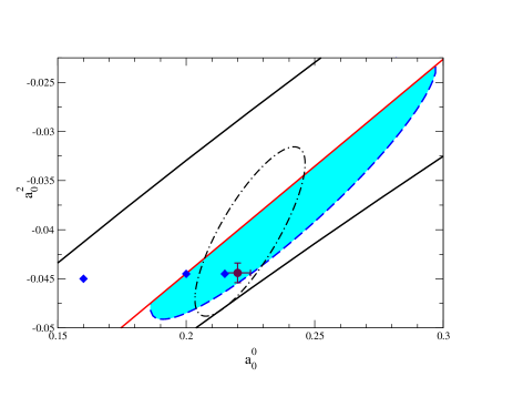
Figure 1: The shaded region represents the intersection of the domains allowed by the old data and by the Olsson sum rule, see [26] for details. The ellipse indicates the impact of the new, preliminary $K_{e_{4}}$ data [28]. The cross shows the result of Ref. [24]. The three diamonds illustrate the convergence of the chiral perturbation series at threshold. The one at the left corresponds to Weinberg’s leading order formulae. The two black solid lines are the boundaries of the universal band [26]

This leads to the following numbers for the chiral expansion of the $I=0$ $S$–wave scattering length:

$$a_{0}^{0}=0.197\;\;O(p^{2})\to 0.2195\;\;O(p^{4})\to 0.220\;\;O(p^{6})\;\;,$$

which show a remarkably fast and good convergence. The difference of this procedure with respect to a direct evaluation of the scattering length is that here the chiral expansion is only applied in the unphysical region, where it converges best – the continuation to threshold to evaluate the scattering length is then provided by the dispersive representation, that, as shown in [26], at low energy does not show significant uncertainties. On this basis, we can safely conclude that yet higher orders will not modify the above predictions beyond the uncertainties present in this matching procedure. Once this are taken into account, the final result for the $S$–wave scattering lengths is

$$\begin{array}[]{ll}a_{0}^{0}=0.220\pm 0.005\,,&\hskip 20.00003pt2a_{0}^{0}-5a_{0}^{2}=0.663\pm 0.006\end{array}$$ (15)

The result (15) relies on the standard picture, according to which the quark condensate represents the leading order parameter of the spontaneously broken symmetry. The scenario investigated in ref.  [30] concerns the possibility that the Gell-Mann–Oakes–Renner formula fails, the second term in the expansion $M_{\pi}^{2}=2\,B\,m\left\{1-\frac{1}{2}\,\xi\,\bar{\ell}_{3}+O(\xi^{2})\right\}$ being of the same numerical order of magnitude or even larger than the first. Note that for this to happen, the value of $|\bar{\ell}_{3}|$ must exceed the estimate we used by more than an order of magnitude. The constraints imposed on $a_{0}^{0}$, $a_{0}^{2}$ by the available experimental information are shown in the figure. The ellipse represents the 68 % confidence level contour obtained by combining the new, preliminary $K_{e_{4}}$ data [28] with earlier experimental results [29]. Concerning the value of $a_{0}^{0}$, the ellipse corresponds to the range $0.2<a_{0}^{0}<0.25$.

The figure shows that the values of $a_{0}^{2}$ and $a_{0}^{0}$ are strongly correlated. The correlation also manifests itself in the Olsson sum rule [31], which according to ref.  [26] leads to $2a_{0}^{0}-5a_{0}^{2}=0.663\pm 0.021+1.13\Delta a_{0}^{0}-1.01\Delta a_{0}^{2}$, in perfect agreement with the result in eq. (15). This combination, however, is not sensitive to $\ell_{3}$ – accurate experimental information in the threshold region is needed to perform a thorough test of the theoretical framework that underlies the calculation. The forthcoming results from Brookhaven [28], CERN [32, 33] and Frascati [34] will provide such a test.

5 Conclusions

We have reviewed recent developments in CHPT, emphasising in particular the problems that arise when pushing the chiral expansion to order $p^{6}$. We have discussed a few examples that show different physical situations: in one case the low–energy constants at order $p^{6}$ have a dominant role, whereas in the other only a marginal one. In the former case CHPT cannot provide a solid prediction with a good control of the uncertainties, whereas in the latter case, it is possible to yield a very precise prediction. The case of $\pi\pi$ scattering has been described in some detail, and we have shown that by combining a dispersive representation and the chiral expansion one can bring the uncertainties down to the few percent level [24].

References

References

- [1] S. Weinberg, Physica A 96, 327 (1979).
- [2] J. Gasser and H. Leutwyler, Ann. Phys. (N.Y.) 158, 142 (1984), and Nucl. Phys. B 250, 465 (1985).
- [3] S. Bellucci, J. Gasser and M. Sainio, Nucl. Phys. B 423, 80 (1994); B 431,413 (1994) (E).
-
[4]
E. Golowich and J. Kambor,
Phys. Rev. D58 (1998) 036004
[hep-ph/9710214].
S. Durr and J. Kambor, Phys. Rev. D61 (2000) 114025 [hep-ph/9907539]. - [5] G. Amoros, J. Bijnens and P. Talavera, hep-ph/9912398; Nucl. Phys. B568 (2000) 319 [hep-ph/9907264].
- [6] J. Bijnens, G. Colangelo and G. Ecker, JHEP 9902 (1999) 020 [hep-ph/9902437]; Annals Phys. 280 (2000) 100 [hep-ph/9907333].
- [7] J. Gasser and H. Leutwyler, Nucl. Phys. B250 (1985) 517.
- [8] D. E. Groom et al., Eur. Phys. J. C15 (2000) 1.
- [9] G. Ecker, J. Gasser, A. Pich and E. de Rafael, Nucl. Phys. B321 (1989) 311.
- [10] R. Urech Nucl. Phys. B 433, 234 (1995); H. Neufeld and H. Rupertsberger Z. Phys. C71, 131 (1996).
- [11] J. Kambor, J. Missimer, and D. Wyler, Nucl. Phys. B 346, 17 (1990); G. Ecker, J. Kambor, and D. Wyler, Nucl. Phys. B 394, 101 (1993).
- [12] G. D’Ambrosio, G. Ecker, G. Isidori and H. Neufeld, in “The Second DANE Physics Handbook”, L. Maiani, G. Pancheri, N. Paver (eds.).
- [13] G. Ecker, A. Pich, and E. de Rafael, Phys. Lett. B 189, 363 (1987); G. Cappiello, and G. D’Ambrosio, Nuovo Cim. 99A, 155 (1988).
- [14] V. Papadimitriou et al. (E731) Phys. Rev. D44, 573 (1991).
- [15] G.D. Barr et al. (NA31) Phys. Lett. B 284, 440 (1992).
- [16] G. Cappiello, and G. D’Ambrosio, and M. Miragliuolo Phys. Lett. B 298, 423 (1993); A. Cohen, G. Ecker, and A. Pich, Phys. Lett. B 304, 347 (1993); J. Kambor, and B.R. Holstein, Phys. Rev. D 49, 2346 (1994).
- [17] G. D’Ambrosio, and J. Portolés, Nucl. Phys. B 492, 417 (1997).
- [18] A.Alavi-Arati et al. (KTeV), Phys. Rev. Lett. 83, 917 (1999).
- [19] J. Bijnens, G. Colangelo and P. Talavera, JHEP 9805, 014 (1998).
- [20] S. Weinberg, Phys. Rev. Lett. 17, 616 (1966).
- [21] J. Gasser and H. Leutwyler, Phys. Lett. B 125, 325 (1983).
- [22] J. Bijnens, G. Colangelo, G. Ecker, J. Gasser and M. Sainio, Phys. Lett. B 374, 210 (1996), Nucl. Phys. B 508, 263 (1997).
- [23] G. Colangelo, Phys. Lett. B 350, 85 (1995); B 361, 234 (1995) (E).
- [24] G. Colangelo, J. Gasser and H. Leutwyler, Phys. Lett. B488 (2000) 261 [hep-ph/0007112].
- [25] S. M. Roy, Phys. Lett. B36 (1971) 353.
- [26] B. Ananthanarayan, G. Colangelo, J. Gasser and H. Leutwyler, hep-ph/0005297.
- [27] M. Knecht, B. Moussallam, J. Stern and N. H. Fuchs, Nucl. Phys. B457 (1995) 513 [hep-ph/9507319]; ibid. B471 (1996) 445 [hep-ph/9512404].
- [28] S. Pislak et al., “A new measurement of ()”, talk at Laboratori Nazionali di Frascati, June 22, 2000.
- [29] L. Rosselet et al. Phys. Rev. D 15, 574 (1977).
- [30] N. H. Fuchs, H. Sazdjian and J. Stern, Phys. Lett. B269 (1991) 183; Phys. Rev. D47 (1993) 3814 [hep-ph/9301244].
- [31] M. G. Olsson, Phys. Rev. 162 (1967) 1338.
- [32] B. Adeva et al., Proposal to the SPSLC, CERN/SPSLC 95-1 (1995).
- [33] R. Batley et al., CERN-SPSC-2000-003.
- [34] M. Baillargeon and P.J. Franzini, in: L. Maiani, G. Pancheri and N. Paver, The Second DANE Physics Handbook (INFN-LNF-Divisione Ricerca, SIS-Ufficio Publicazioni, Frascati, 1995), p. 413 [hep-ph/9407277].