THE INITIAL STATE OF ULTRA-RELATIVISTIC HEAVY ION COLLISION
V.K. Magas1,⋆, L.P. Csernai1,2,⋆ and D.D. Strottman 3,4,⋄
1 Section for Theoretical and Computational Physics, Department of Physics
University of Bergen, Allegaten 55, N-5007, Norway
2 KFKI Research Institute for Particle and Nuclear Physics
P.O.Box 49, 1525 Budapest, Hungary
3 Theoretical Division, Los Alamos National Laboratory
Los Alamos, NM, 87454, USA
4 Institut für Theoretische Physik, Universität Frankfurt
Robert-Mayer-Str. 8-10, D-60054 Frankfurt am Main, Germany
A model for energy, pressure and flow velocity distributions at the beginning of ultra-relativistic heavy ion collisions is presented, which can be used as an initial condition for hydrodynamic calculations. Our model takes into account baryon recoil for both target and projectile, arising from the acceleration of partons in an effective field, , produced in the collision. The typical field strength (string tension) for RHIC energies is about , what allows us to talk about ”string ropes”. The results show that a QGP forms a tilted disk, such that the direction of the largest pressure gradient stays in the reaction plane, but deviates from both the beam and the usual transverse flow directions. Such initial conditions may lead to the creation of ”antiflow” or ”third flow component” [28]. PACS numbers: 25.75.-q, 24.85.+p, 25.75.Ld, 24.10.Jv.
I Introduction
Fluid dynamical models are widely used to describe ultra-relativistic heavy ion collisions. Their advantage is that one can vary flexibly the Equation of State (EoS) of the matter and test its consequences on the reaction dynamics and the outcome. For example, the only models which may handle the supercooled QGP are hydrodynamical models with corresponding EoS. In energetic collisions of large heavy ions, especially if a Quark-Gluon Plasma (QGP) is formed in the collision, one-fluid dynamics is a valid and good description for the intermediate stages of the reaction. Here, interactions are strong and frequent, so that other models, (e.g. transport models, string models, etc., that assume binary collisions, with free propagation of constituents between collisions) have limited validity. On the other hand, the initial and final, Freeze-Out (FO), stages of the reaction are outside the domain of applicability of the fluid dynamical model.
Thus, the realistic, and detailed description of an energetic heavy ion reaction requires a Multi Module Model, where the different stages of the reaction are each described with a suitable theoretical approach. It is important that these Modules are coupled to each other correctly: on the interface, which is a three dimensional hyper-surface in space-time with normal , all conservation laws should be satisfied, e.g. (here the square brackets means difference between new and old phases or modules), and entropy should not decrease, . These matching conditions were worked out and studied for the matching at FO in detail in Refs. [1, 2, 3, 4, 5, 6].
We would like to discuss the entropy condition in more detail. Obviously, the number of degrees of freedom and correspondingly the entropy density is reduced during hadronization process. So, how can we avoid decreasing of the entropy? Two scenarios have been proposed. The first one is the gradual hadronization scenario i.e., the hadronization is so slow that during this process the volume of the system becomes considerably larger to compensate for the reduction of entropy density. If this would be so, our long living, gradually expanding QGP should be observed in HBT experiments, e.g., as a peak in the ratio [7]. The preliminary data from STAR and PHENIX do not support this scenario [8]. The second possibility is the fast hadronization from supercooled QGP [9]. This hypothesis can be checked only in hydrodynamical models, which use the EoS as direct input.
After hadronization and FO, matter is already dilute and can be described well with kinetic models.
The initial stages are more problematic. Frequently, two or three fluid models are used to remedy the difficulties and to model the process of QGP formation and thermalization [10, 11, 12]. Here the problem is transferred to the determination of drag-, friction- and transfer- terms among the fluid components, and a new problem is introduced with the (unjustified) use of an EoS in each component in a nonequilibrated situations where an EoS is not defined. Strictly speaking this approach can only be justified for mixtures of noninteracting ideal gas components. Similarly, the use of transport theoretical approaches assuming dilute gases with binary interactions is questionable, as, due to the extreme Lorentz contraction in the Center of Mass (CM) frame, enormous particle and energy densities with the immediate formation of a perturbative vacuum should be handled. Even in most parton cascade models these initial stages of the dynamics are just assumed in form of some initial condition, with little justification.
Our goal in the present work is to construct a model, based on the recent experiences gained in string Monte Carlo models and in parton cascades. One important conclusion of heavy ion research in the last decade is that standard ’hadronic’ string models fail to describe heavy ion experiments.
All string models had to introduce new, energetic objects: string ropes [13, 14], quark clusters [15], or fused strings [16], in order to describe the abundant formation of massive particles like strange antibaryons. Based on this, we describe the initial moments of the reaction in the framework of classical (or coherent) Yang-Mills theory, following Ref. [20] assuming a larger field strength (string tension) than in ordinary hadron-hadron collisions. For example, calculations both in the Quark Gluon String Model (QGSM) [17, 18, 19] and in the Monte Carlo string fusion model [16] indicate that the energy density of strings reaches already in SPS reactions, nearly times more than the tension used in standard, ’hadronic’, string models where . In addition we now satisfy all conservation laws exactly, while in Ref. [20] infinite projectile energy was assumed, and so, overall energy and momentum conservation was irrelevant. Thus, in this approach for the first time the initial transparency/stopping and energy deposited into strings and ”string ropes” will be determined consistently with each other. Recent parton kinetic models [21, 22] indicate that quark and gluon density saturation takes place in a very short time - for LHC - SPS energies [22], and pressure needs to be established [21]. More importantly the first experiments at RHIC yield strong elliptic flow, which cannot be reproduced in any other model, except in fluid dynamical models with QGP EoS [23]. This is a strong experimental indication that transverse pressure builds up early in these reactions, in a few , and strong stopping is also necessary to create strong flow before Freeze Out, which usually happens when the system size is not more than . We present initial conditions for , which is in agreement with previous estimations as well as with data.
We do not solve simultaneously the kinetic problem leading to parton equilibration, but assume that the arising friction is such that the heavy ion system will be an overdamped oscillator, i.e., yo-yoing of the two heavy ions will not occur, as all recent string and parton cascade results indicate.
II Formulation of model
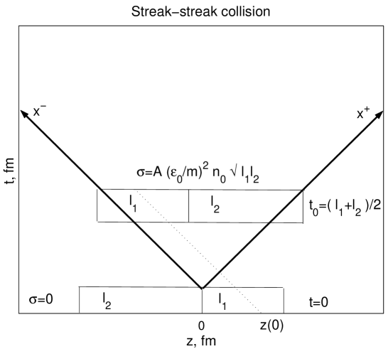
Our basic idea is to generalize the model developed in [20] for collisions of two heavy ions and improve it by strictly satisfying conservation laws [24, 25, 26]. First of all, we would create a grid in the plane ( is the beam axes, is the reaction plane). We will describe the nucleus-nucleus collision in terms of steak-by-streak collisions, corresponding to the same transverse coordinates, . We assume that baryon recoil for both target and projectile arise from the acceleration of partons in an effective field , produced in the interaction. Of course, the physical picture behind this model should be based on chromoelectric flux tube or string models, but for our purpose we consider as an effective Abelian field. The most important consequence of the non-Abelian fields, i.e., its self interaction and the resulting flux tubes of constant cross section, are, nevertheless, reflected in our model: assuming that the field is one-dimensional. The fields generated by the colliding streaks are of constant cross section during the whole evolution, and only their lengths increase with time. As the string tension is constant, the energy of the string increases linearly with its increasing length. The single phenomenological parameter we use to describe this field must be fixed from comparison with experimental data.
We describe the streak-streak collision using conservation laws:
| (1) |
| (2) |
where is the baryon current of th nucleus, is the color charge and it will be discussed in more detail later. We are working in the Center of Rapidity Frame (CRF), which is the same for all streaks. The concept of using target and projectile reference frames has no advantage any more. We will use the parameterization:
| (3) |
is the energy-momentum flux tensor. It consists of five parts, corresponding to both nuclei and free field energy (also divided into two parts) and one term defining the QGP perturbative vacuum.
| (4) |
Here is the bag constant, the equation of state is , where and are energy density and pressure of QGP.
Within each streak we form only one flux tube with a uniform field strength or field tension, , from the target to the projectile. For practical purposes we, however, divide this field into two spatial domains, a target and a projectile domain, (), separated at a fixed point, , so that . The choice if this point will be specified later. (The field is constant and the only change is that it extends with time at its two ends.)
In complete analogy to electro-magnetic field
| (5) |
| (6) |
| (7) |
| (8) |
In our case the string tensions, , will be constant in the space-time region after string creation and before string decay. The creation of fields will be discussed later in more detail.
To get the analytic solutions of the above equations, we use lightcone variables
| (9) |
Following [20], we insist that are functions of only and depend on only.
In terms of lightcone variables:
| (10) |
| (11) |
where
| (12) |
The other tensors in the light cone variables are:
| (13) |
| (14) |
The energy-momentum tensor for free field in the light cone variables is:
| (15) |
At the time of the first touch of two streaks, , there is no string tension. We assume that strings are created, i.e., the sting tension achieves the value at time , corresponding to complete penetration of streaks through each other (see Fig. 1).
III Conservation laws and string creation
In lightcone variables eq. (2) may be rewritten as
| (16) |
So, we have a sum of two terms, each depending on different independent variables, and the solution can be found in the following way:
| (17) |
where the index indicates the initial proper density, which is the normal nuclear density: . Since both and are positive (and also more or less symmetric) we can conclude that for our case .
Finally
| (18) |
| (19) |
where is the initial rapidity of nucleus in the center of rapidity frame (CRF), respectively. The other components are given by eq. (10).
Let us make analogy to electro-magnetic field, where two charges and move in the opposite directions, creating string-like field between them, , which is constrained transversally into a constant cross section. The Z-axis goes through charges and and directed from to (let us assume that we have such a field configuration). So, forces acting on our charges, and , have opposite sign and both are working against the expansion of the ”string”. In our effective model we use color charges, and assume that the vectors of these color charges point in the opposite directions in the color space [16], so that the forces acting on both target and projectile partons are opposite both stopping the expansion of the streak. As our field strength (string tension, ) is not yet defined we normalize the charges to unity:
| (20) |
Then we have the forces acting in direction: and . Notice again that after string creation fields and are spatially separated as well as the baryon densities, and ; i.e., after complete penetration of the initial streaks through each other (see Fig. 1), acts on the partons on the right side of the separating point , while the acts on those on the left side. In the absence of matter, in the middle both fields are identical, so the exact position of the separating point does not play any role until it does not enter the target or projectile matter. The fields and are generated by the corresponding 4-potentials , which are different and spatially separated in the same way.
As it was described above we do not generate the chromo-electric field self consistently, as a product of color currents, which a affected also by the field. Our effective fields are external with respect to colliding partons, that why we can use the expression (15) for the field energy. On the other hand, if we want to satisfy the conservation laws, we must generate our effective fields in the collision transferring energy from matter to field. It’s possible to define new conserved quantities based on eq. (1). Using the definition of , eq. (6), we can rewrite eq. (1) as
| (21) |
The solutions for and , eq. (18), show that the second term vanishes. The fourth term is a vector in lightcone coordinates. So, if we impose the conditions
| (22) |
we can define a new energy-momentum tensor , such that
| (23) |
| (24) |
To satisfy the above choice of the fields, (20), and imposed conditions (22) together with the Lorentz gauge condition, or , we take the vector potentials in the following form:
| (25) |
Notice that the above choice differs from the one which was initially proposed in Refs. [24, 25, 26], what causes the changes in the expressions related to field creation in this section - eqs. (27,31,32) - but will not affect the analytic solution of the model - eqs. (34-38).
In our calculations we used the parameterization:
| (26) |
where is the nucleon mass, and and are the initial streak lengths (see Fig. 1). We are working in the system, where , so has a dimension of . The typical values of dimensionless parameter are around . Notice, that there is only one free parameter in parameterization (26). The typical values of are for per nucleon, and for per nucleon. These values are consistent with the energy density in non-hadronized strings, or ”latent energy density” which is on the average [17, 18, 19].
Using the exact definition of , eqs. (25), eqs. (11,14,15,20,24) and transformation matrixes from Appendix C we obtain
| (27) |
Notice that perturbative term, , and free field energy, , cover all the interacting volume, while energy densities of matter and baryon currents are separated in space. We also want to stress factor in front of all terms in (it has been canceled by near in last two terms) - this factor was missed in Refs. [24, 25, 26] as well as in [20], although it does not affect the result since equations of motion, , can be multiplied by any coefficient. The reason for it is a form of transformation matrixes between and coordinates, which are presented in Appendix C.
Now the new conserved quantities are
| (28) |
| (29) |
where the volume integral runs over the lengths of the both streaks and is the cross section of the streaks. Notice that in the absence of the fields, before string creation and after string decay, the come back to - components of the 4-momenta of the system.
We can rewrite energy-momentum tensor in coordinates:
| (30) |
Based on conservation of we can calculate energy densities, , at the moment , when the string with tension is created. These new quantities are used as initial conditions for our differential eqs. (1, 2). As shown in Appendix A –
| (31) |
| (32) |
Here the is a proper energy density at the time , is the initial energy per nucleon. We assumed transparency, i.e., that complete penetration happened so fast, that the fields, created during this time, did not have time to stop partons. So, the rapidities are correspondingly, and the proper baryon densities did not change.
For we should solve eqs. (23), with boundary conditions
| (33) |
where defines the string creation surface , for parton or cell element in the position at the time .
Let us present the complete analytical solution in the following form (for detailed calculations see Appendix B)
| (34) |
| (35) |
| (36) |
where , , and the notations are from Appendix B (B.7,B.9,B.13-B.15).
Then the trajectories of partons (or cell elements) for both nuclei are given by:
| (37) |
| (38) |
for parton or cell element in the position at the time .
IV Recreation of matter
If we let partons (or cell domains) evolve according to the above trajectories, eqs. (37, 38), they will keep going in the initial direction up to the time , then they will turn and go backwards until the two streaks again penetrate through each other and a new oscillation will start. Such a motion is analogous to the ”Yo-Yo” motion in the string models. Of course, it is difficult to believe that such a process would really happen in heavy ion collisions, because of string decays, string-string interactions, interaction between streaks and other reasons, which would be difficult to take into account. To be realistic we should stop the motion described by eqs. (37, 38) at some moment before the projectile and target cross again.
We assume that the final result of collisions of two streaks, after stopping the string’s expansion and after its decay, is one streak of the length with homogeneous energy density distribution, , and baryon charge distribution, , moving like one object with rapidity . We assume that this is due to string-string interactions and string decays. As was mentioned above the typical values of the string tension, , are of the order of , and these may be treated as several parallel strings. The string-string interaction will produce a kind of ”string rope” between our two streaks, which is responsible for final energy density and baryon charge distributions. For simplicity we assume homogeneous baryon charge distribution. Notice, that in this way, after the decay of our ”string rope” charges do not remain at the ends of the final streak, as it would be if we assume full transparency. The real situation may be more complicated: when the energy accumulated in the strong color fields will be finally released in a production of pairs and gluons, this process may noticeably change composition of matter as compared to the chemical equilibrium case [27]. Therefore, matter created after the mutual stopping of interpenetrating streaks can not, in general, be described by the equilibrium EoS. The homogeneous distributions are the simplest assumptions, which may be modified later based on experimental data. Its advantage is a simple expression for . The first experimental results from RHIC do not show transparency, rather most particle multiplicities as well as the elliptic flow show strong stopping and a peak around mid rapidity [23]. Furthermore, we describe the initial state, which is not directly observable in experiments, and a flat initial rapidity distribution may end up in both a forward-backward peaked and a centrally peaked distributions depending on several other circumstances.
The final energy density, baryon density and rapidity, and , should be determined from conservation laws. The assumptions we made above oversimplify the situation, and do not allow us to satisfy exactly all conservation laws. The reason for this is well known and has been discussed in the Refs. [2, 3, 4, 5, 6]: two possible definitions of the flow, Eckart’s and Landau’s definition. If we are following the energy flow, we satisfy exactly the energy and momentum conservation, but violate the net baryon current conservation. (Otherwise, if we were to choose baryon flow, we would violate the energy-momentum conservation.)
The exact conservation of the energy and momentum gives for the final rapidity:
| (39) |
where we neglected next to and introduced the notation , is the initial velocity. (The exact conservation of the baryon four-current would give: , ).
It is interesting to analyze these equations, as functions of and . If or then , and . To calculate this limit for we should put , since we do not have collisions and, consequently, do not create QGP, thus . So there is no stopping as expected, because there is no reason to stop. If and both expressions give , i.e., complete stopping. So, we see that Landau’s and Eckart’s expressions behave similarly, have the same limits for minimal and maximal stopping.
For the following part of this work we choose Landau’s convention, , which is justifiable for RHIC and SPS energies, where the evolution of matter is not dominated by the net baryon charge, unlike at lower energies where the baryon mass is still dominant and pair creation is of little importance.
In this case the expressions for the and are:
| (40) |
| (41) |
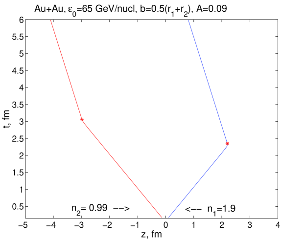
The typical trajectory of the streak-ends is presented in Fig. 2. From they move according to eqs. (37, 38) until they reach the rapidity . Later the final streak starts to move like one object with uniform rapidity, , until we reach the time when the fluid dynamical calculation starts.
The time and position of final streak formation can be found from the condition:
| (42) |
which gives for the th nucleus ()
| (43) |
V Initial conditions for hydrodynamic calculations
In this section we present the results of our calculations. We are interested in the shape of the QGP formed when string expansions stop and their matter is locally equilibrated. This will be the initial state for further hydrodynamic calculations. The time, , at which we assume the system to reach overall local equilibrium and to start hydrodynamic description, is a second (after ) free parameter of our model. Of course, should be larger than the time of final streak formation, at least in the central most hot and dense region. For the peripheral streaks the string tension is low, and the transparency is large, but peripheral matter does not play a leading role in further hydrodynamic expansion. So, to have a homogeneous output for each streak-streak collision, we will also build the final streaks () for peripheral streak-streak collisions, with lengths, , corresponding the lengths of the interacting region at the moment , even if the final rapidity, , was not yet achieved for this particular collision.
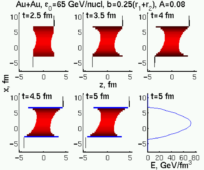
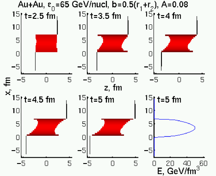
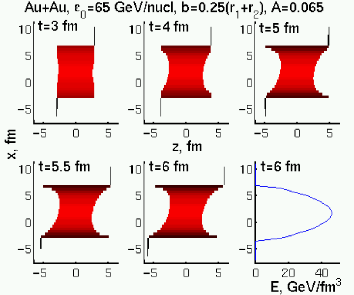
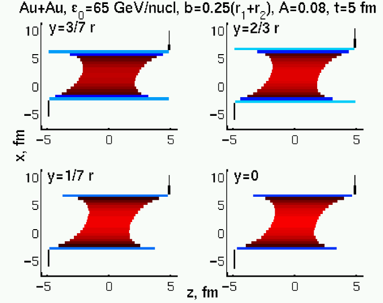
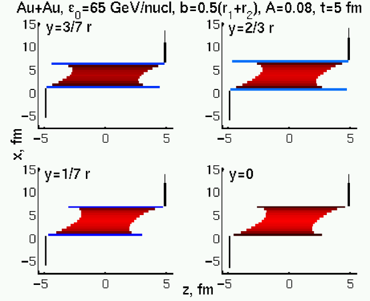
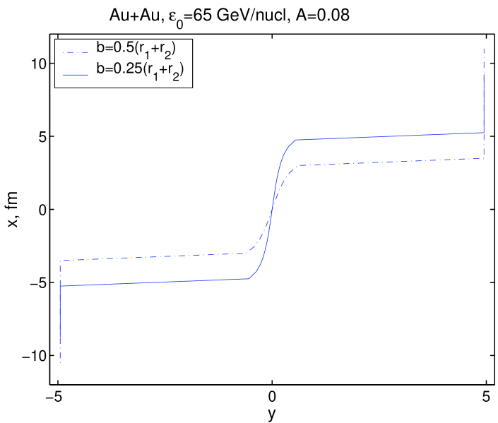
We may see in Figs. 3, 4, 5, 6 that finally a QGP forms a tilted disk for . Thus, the direction of fastest expansion, the same as largest pressure gradient, will be in the reaction plane, but will deviate from both the beam axis and the usual transverse flow direction. So, the new flow component, called ”antiflow” or ”third flow component” [28], will appear in addition to the usual transverse flow component in the reaction plane. With increasing beam energy the usual transverse flow is getting weaker, while this new flow component is strengthened. The mutual effect of the usual directed transverse flow and this new ”antiflow” or ”third flow component” contribute to an enhanced emission in the reaction plane. This was actually observed and studied earlier. One should also mention that both the standard transverse flow and new ”antiflow” contribute to ”elliptic flow”.

The last subplots in the Figs. 3, 4, 5, 6 present the energy density distribution in the laboratory frame, for . It seems to be bigger than what one can expect from estimation based on the Bjorken model. One should, nevertheless, keep in mind that our ”fireball” is not homogeneous in plane. The average energy density for the equivalent homogeneous ”fireball” would be lower - . Other hydrodynamical models had to use similarly high initial energy density to reproduce the observed flow, e.g. in [29] has been used.
VI Conclusions
Based on earlier Coherent Yang-Mills field theoretical models and introducing effective parameters, based on Monte-Carlo string cascade and parton cascade model results, a simplified model is introduced to describe the pre fluid dynamical stages of heavy ion collisions at the highest SPS energies and above. The model predicts limited transparency for massive heavy ions.
Contrary to earlier expectations — based on standard string tensions of which lead to the Bjorken model type of initial state — effective string tensions are introduced for collisions of massive heavy ions. The increased string tension is a consequence of collective effects related to QGP formation. These collective effects in central and semi central collisions lead to an effective string tension of the order of and consequently cause much less transparency than earlier estimates. The resulting initial locally equilibrated state of matter in semi central collisions takes a rather unusual form, which can be then identified by the asymmetry of the caused collective flow. Our prediction is that this special initial state may be the cause of the recently identified ”antiflow” or ”third flow component”.
Detailed fluid dynamical calculations as well as flow experiments at semi central impact parameters for massive heavy ions are needed at SPS and RHIC energies to connect the predicted special initial state with observables.
Acknowledgment
One of the authors (D.D.S.) thanks the support of the Bergen Computational Physics Laboratory in the framework of the European Community - Access to Research Infrastructure action of the Improving Human Potential Programme and the Humboldt Foundation.
Appendix A : Initial conditions after string creation
Our conserved quantities are (28,29)
| (A.1) |
| (A.2) |
and are given by eq. (30). Before string creation the initial values of the modified energy-momentum tensor, , are
| (A.3) |
| (A.4) |
where is the nucleon mass, is the initial energy per nucleon, and we have used . is the initial velocity, is a good approximation for ultra-relativistic heavy ion collisions. So,
| (A.5) |
| (A.6) |
where and are the initial lengths of streaks (see Fig 1), , are the grid sizes in and directions.
After string creation
| (A.7) |
| (A.8) |
At the point of complete penetration of streaks, (see Fig 1), we introduced energy densities and . We assumed transparency, i.e., that complete penetration happened so fast, that field, itself created during this time, did not have time to stop partons. So, the rapidities correspondingly, and the proper baryon densities did not change, and, thus, the baryon current conserved automatically. This assumption differs from how it was done in Refs. [24, 25, 26], but they seems to be more physical, and do not change final results very much. Terms proportional to can be neglected. Then the energy and momentum conservation laws can be written in the form:
| (A.9) |
| (A.10) |
Appendix B : The analytical solution of the model
For we should solve eqs. (23), based on boundary conditions (33). Eqs. (23) leads to the system of equations:
| (B.1) |
| (B.2) |
where . It is clear, that in both equations there are two terms depending on independent variables, so the solution will contain two undefined constants. The next step is to take eqs. (B.1, B.2) at the values and .
| (B.3) |
| (B.4) |
| (B.5) |
| (B.6) |
where we introduced new notations
| (B.7) |
and two new constants
| (B.8) |
which will be estimated by assuming a linear development for the enthalpy densities, and , from to .
| (B.9) |
The complete analytical solution found to be
| (B.10) |
| (B.11) |
| (B.12) |
where , ,
| (B.13) |
| (B.14) |
| (B.15) |
Appendix C : Transformation to the lightcone coordinates
In this Appendix we present the transformation matrixes between and coordinates. Indexes run for , indexes are used for .
The transformation of the coordinate system is
| (C.1) |
thus, for all contravariant vectors we have the same:
| (C.2) |
For coordinates we have
| (C.3) |
Then
| (C.4) |
| (C.5) |
| (C.6) |
| (C.7) |
so,
| (C.8) |
| (C.9) |
| (C.10) |
| (C.11) |
The backward transformation is
| (C.12) |
so,
| (C.13) |
| (C.14) |
| (C.15) |
| (C.16) |
REFERENCES
- [1] L.P. Csernai, Zs. Lázár and D. Molnár, Heavy Ion Phys. 5 (1997) 467.
- [2] Cs. Anderlik, Z.I. Lázár, V.K. Magas, L.P. Csernai, H. Stöcker and W. Greiner, Phys. Rev. C 59 (1999) 388. (nucl-th/9808024)
- [3] Cs. Anderlik, L.P. Csernai, F. Grassi, W. Greiner, Y. Hama, T. Kodama, Zs. Lazar, V. Magas and H. Stoecker, Phys. Rev. C 59 (1999) 3309. (nucl-th/9806004)
- [4] V.K. Magas, Cs. Anderlik, L.P. Csernai, F. Grassi, W. Greiner, Y. Hama, T. Kodama, Zs. Lázár and H. Stöker, Heavy Ion Phys. 9 (1999) 193. (nucl-th/9903045)
- [5] Cs. Anderlik, L.P. Csernai, F. Grassi, W. Greiner, Y. Hama, T. Kodama, Zs. Lazar, V. Magas and H. Stoecker, Phys. Lett. B 459 (1999) 33. (nucl-th/9905054)
- [6] V.K. Magas, Cs. Anderlik, L.P. Csernai, F. Grassi, W. Greiner, Y. Hama, T. Kodama, Zs. Lázár and H. Stöker, Nucl. Phys. A 661 (1999) 596. (nucl-th/0001049)
- [7] D.H. Rischke, M. Gyulassy, Nucl. Phys. A608 (1996) 479.
- [8] F. Laue, talk at the Quark Matter 2001, Stony Brook, Janyary 15-20, 2001; S. Johnson, talk at the Quark Matter 2001, Stony Brook, Janyary 15-20, 2001; S. Panitkin, talk at the Quark Matter 2001, Stony Brook, Janyary 15-20, 2001.
- [9] L.P. Csernai, I.N. Mishustin, Phys. Rev. Lett. 74 (1995) 5005.
- [10] A.A. Amsden, A.S. Goldhaber, F.H. Harlow and J.R. Nix, Phys. Rev. C17 (1978) 2080.
- [11] L.P. Csernai, I. Lovas, J. Maruhn, A. Risenhauer, J. Zimanyi, W. Greiner, Phys. Rev. C26 (1982) 149.
- [12] J. Brachmann, S. Soff, A. Dumitru, H. Stöker, J.A. Maruhn, W. Greiner, D.H. Rischke, L. Bravina, Phys. Rev. C61 (2000) 024909.
- [13] T.S. Biró, H.B. Nielsen, J. Knoll, Nucl. Phys. B245 (1984) 449.
- [14] H. Sorge, Phys. Rev. C52 (1995) 3291.
- [15] K. Werner, J. Aichelin, Phys. Rev. Lett. 76 (1996) 1027.
- [16] N.S. Amelin, M.A. Braun, C. Pajares, Phys. Lett. B306 (1993) 312, Z. Phys. C63 (1994) 507.
- [17] N. S. Amelin, E.F. Staubo, L.P. Csernai, V.D. Toneev, K.K. Gudima and D.D. Strottman, Phys. Lett. B261 (1991) 352.
- [18] N. S. Amelin, E.F. Staubo, L.P. Csernai, V.D. Toneev, K.K. Gudima and D.D. Strottman, Phys. Rev. Lett. 67 (1991) 1523.
- [19] N.S. Amelin, L.P. Csernai, E.F. Staubo, and D. Strottman Nucl. Phys. A544 (1992) 463c.
- [20] M. Gyulassy, L.P. Csernai, Nucl. Phys. A460 (1986) 723.
- [21] K.J. Eskola, K. Kajantie, P.V. Ruuskanen, K. Tuominen, Nucl. Phys. B570 (2000) 379.
- [22] A. Dumitru, M. Gyulassy, Phys. Lett. B 494 (2000) 215.
- [23] P. Steinberg, talk at the Quark Matter 2001, Stony Brook, Janyary 15-20, 2001; R. Snellings, talk at the Quark Matter 2001, Stony Brook, Janyary 15-20, 2001; A. Drees, talk at the Quark Matter 2001, Stony Brook, Janyary 15-20, 2001.
- [24] V.K. Magas, L.P. Csernai, D.D. Strottman, Proceedings of New Trends in High-Energy Physics, Yalta (Crimea), Ukraine, May 27 - June 4, 2000, p. 93. (nucl-th/0009049)
- [25] L.P. Csernai, Cs. Anderlik, V.K. Magas, presented at the Symposium on Fundamental in Elementary Matter, Bad Honnef, Germany, September 25-29, 2000. (nucl-th/0010023)
- [26] V. Magas, L.P. Csernai, D. Strottman, presented at the ISMD 2000 - XXXth International Symposium on Multiparticle Dynamics, Tihany, Lake Balaton, Hungary, October 9-15, 2000. (hep-ph/0101125)
- [27] K. Kajantie, T. Matsui, Phys. Lett. B164 (1985) 373.
- [28] L.P. Csernai, D. Röhrich, Phys. Lett. B458 (1999) 454. (nucl-th/9908034)
- [29] P. Huovinen, talk at the Quark Matter 2001, Stony Brook, Janyary 15-20, 2001.
- [30] R.J.M. Snellings, H. Sorge, S.A. Voloshin, F.Q. Wang, N. Xu, Phys. Rev. Lett. 84 (2000) 2803-2805. (nucl-ex/9908001)