The Prompt Lepton Cookbook

Abstract

We review the calculation of the prompt lepton flux, produced in the atmosphere by the semileptonic decay of charmed particles. We describe side by side the intermediary ingredients used by different authors, which include not only the charm production model, but also other atmospheric particle showering parameters. After evaluating separately the relevance of each single ingredient, we analyze the effect of different combinations over the final result. We highlight the impact of the prompt lepton flux calculation upon high-energy neutrino telescopes.

1 Introduction

Very-high-energy (above 1 TeV) neutrino astronomy is currently a subject of great interest, promising to expand our observational range of the Universe in an unique way[1]. Such energetic neutrinos may carry information from the sources of the highest energy phenomena ever observed in cosmic rays, possibly coming from active galactic nuclei (AGN) or gamma ray bursts (GRB). They may probe the early stages of the Universe and its farthest distances. In addition, they will contribute to the search of weakly interacting massive particles (WIMP), supernova explosions, monopoles, besides the discovery potential for new physics, which we can even not imagine yet. Neutrino telescopes under development, like the Antarctic Muon and Neutrino Detector Array (AMANDA) and the experiment at Lake Baikal, are already operational, and producing their first results[2, 3]. In addition, great activity is planned for the near future[4].

Aside from these perspectives, the operation of a neutrino detector at energies above 1 TeV poses challenging difficulties. One of the major limitations in the detection of a cosmic high-energy neutrino (from galactic or extra-galactic origin) is the background from atmospheric muons and neutrinos (produced by the interaction of high-energy cosmic rays in the atmosphere).

The source of the atmospheric neutrino background changes with energy, in a way governed by the critical energy $\varepsilon_{critic}$ of the parent particle. This is the energy for which the decay and interaction lengths are equal. Above this energy the parent particle is likely to interact or be slowed down before decaying into a neutrino. The critical energy is calculated in terms of the particle rest energy $mc^{2}$, the mean life $\tau$ and, by adopting the isothermal atmosphere approximation, a scale constant $h_{o}$[5]:

$$\varepsilon_{critic}\>=\>\frac{mc^{2}}{c\tau}\>h_{o}.$$ (1)

Table 1 summarizes several particle properties, derived from the Review of Particle Physics [6]. Comparing the critical energies we observe that muon decays contribute substantially to the atmospheric lepton flux only up to a few GeV’s, while the decays in flight of charged pions and kaons are still important up to about 1-10 TeV. They give rise to the “conventional” atmospheric lepton flux. Above this energy range, the semileptonic decay of very-short lived charmed particles (mainly $D$-mesons and $\Lambda_{c}^{+}$-hyperons) is the dominant source, despite their low production rate. The main contribution comes from the decay modes

$$D\rightarrow K+\mu+\nu\>\>{\rm and}\>\>\Lambda_{c}\rightarrow\Lambda_{o}+\mu+\nu.$$

Muons and neutrinos thus generated are called “prompt leptons”, and they exhibit a flatter (and thus harder) energy spectrum. The lack of precise information on high-energy charm production in hadron-nucleus collisions leads to a great uncertainty in the estimate of the leptonic flux above 100 TeV. In addition, different authors do not use the same atmospheric particle showering routines, turning the comparison even more difficult. The predictions of resulting fluxes span up to four orders of magnitude!

It is our purpose to bring some light to the forum of prompt lepton fluxes, describing side by side the many ingredients of the calculation. After evaluating separately the relevance of each single shower parameter, we analyze the effect of different combinations over the final result. We investigate the fluxes of $\mu$, $\nu_{\mu}$ and $\nu_{e}$, leaving the case of $\tau$ and $\nu_{\tau}$ for a further work.

Table 1: Particle data summary.

Particle	Elementary	$mc^{2}$	$c\tau$	$\varepsilon_{critic}$(1)	Branching
	contents	(MeV)		(GeV)	ratio $B_{i}$(2)
$D^{+},D^{-}$	$c\bar{d},\bar{c}d$	1870	317 $\mu$m	$3.8\times 10^{7}$	17.2 %
$D^{o},\bar{D}^{o}$	$c\bar{u},\bar{c}u$	1865	124 $\mu$m	$9.6\times 10^{7}$	6.8 %
$D_{s}^{+},D_{s}^{-}$	$c\bar{s},\bar{c}s$	1969	149 $\mu$m	$8.5\times 10^{7}$	5.2 %
$\Lambda_{c}^{+}$	$udc$	2285	62 $\mu$m	$2.4\times 10^{8}$	4.5 %
$\mu^{+},\mu^{-}$	lepton	106	659 m	1.0	100 %
$\pi^{+},\pi^{-}$	$u\bar{d},\bar{u}d$	140	7.8 m	115	100 %
$K^{+},K^{-}$	$u\bar{s},\bar{u}s$	494	3.7 m	855	63.5 %
$\Lambda^{o}$	$uds$	1116	7.9 cm	$9.0\times 10^{4}$	0.1 %
(1) According to Eq. (1), with $h_{o}=6.4$ km.
(2) For inclusive decays yielding leptons.

2 Calculation of the prompt lepton flux

The calculation of the prompt lepton flux has been carried out in the past (see, e.g. Ref.[7] and references therein), mainly with the purpose to investigate the effects of choosing a different charm production model. The outline of the calculation is basically the same in all of these works. We start from the primary cosmic ray flux at the top of the atmosphere, with a composition supposed to be dominated by protons, and evaluate the flux of nucleons at any atmospheric depth. Those nucleons interact with the nuclei of air to produce secondary particle showers. For energies above a few TeV, the secondary particles of interest to be followed are the charmed hadrons, for they will be the main source of high energy atmospheric leptons. We will, therefore, consider the contribution of mesons $D^{\pm},D^{o}$ and $\bar{D}^{o}$ (comprising in the same notation the overall contribution of $D$ and $D^{*}$ mesons), of the strange $D_{s}^{\pm}$ and of the $\Lambda_{c}^{+}$-hyperon.

Because the production rate of the mesons $D_{s}$ is relatively lower (about $20\%$ of the $D$ production cross section), some authors neglect their contribution, although their critical energy and branching ratio are comparable to those of the other charmed particles (see Table 1). When calculating the flux of $\tau$ and $\nu_{\tau}$, which we do not consider in this analysis, the role of $D_{s}$ turns out to be mostly important[8].

It is straightforward to calculate the flux of charm particles at any depth, and they will promptly decay yielding electrons, muons and neutrinos. We may integrate the flux for all possible charmed parent production and decay depths, and for all possible production and decay energies, leading to the flux of a chosen lepton at a given depth and energy.

For detailed calculations we refer to Refs.[7, 9, 10], and we follow the notation of the latter, to present here only main results. Let’s write the primary cosmic-ray spectrum as a power law in energy:

$$\Phi_{N}(E_{N},x=0)\>=\>N_{o}\>E_{N}^{-(\gamma+1)},$$ (2)

where $\Phi_{N}(E_{N},x)$, given in (GeV.cm².s.sr)^-1, is the differential flux of nucleons with energy $E_{N}$, in GeV, and $x$ is the slant depth penetrated by the cascade, measured in g/cm² from the top of the atmosphere ($x=0$) downward along the direction of the incident nucleon. The constant $N_{o}$ is the amplitude, or differential spectrum normalization; and $\gamma$ is the spectral index, or slope of the integral primary spectrum.

After developing to a certain depth $x$, the nucleonic flux is given in terms of $\Lambda_{N}$, the nucleonic attenuation length[5]:

$$\Phi_{N}(E_{N},x,\theta)\>=\>N_{o}\>E_{N}^{-(\gamma+1)}\>e^{-x/\Lambda_{N}}.$$ (3)

The resulting flux of secondary particles of type-$i$ ($i=D^{\pm},D^{o},\bar{D}^{o},D_{s}^{\pm},\Lambda_{c}^{+}$) is calculated by convolution of the nucleonic flux with the production spectrum of secondary particles:

$$\Phi_{i}(E_{i},x,\theta)\>=\>K_{i}(E_{i},\gamma)\>\int_{0}^{x}dx^{\prime}\>\left(\frac{x^{\prime}}{x}\right)^{\eta}\>\exp\left\{-\frac{(x-x^{\prime})}{\lambda_{i}}\>-\frac{x^{\prime}}{\Lambda_{N}}\right\},$$ (4)

defining

$$\eta\>=\>\frac{\varepsilon_{critic}}{E_{i}\>\cos\!\theta},$$

where the dependence in the zenith angle holds for $\theta\leq 60^{o}$. For higher zenith angles the curvature of Earth must be taken into account. Both the nucleonic attenuation length $\Lambda_{N}$ and the charmed particle interaction length $\lambda_{i}$ are given in units g/cm². The production spectrum of charmed particles, weighted by the primary nucleonic spectrum, is written as:

$$K_{i}(E_{i},\gamma) = \int_{E_{i}}^{\infty}dE_{N}\>\>\frac{N_{o}}{\lambda_{N}}\>E_{N}^{-(\gamma+1)}\>\frac{dW^{Ni}(E_{i},E_{N})}{dE_{i}},$$ (5)

$$= \frac{N_{o}}{\lambda_{N}}\>E_{i}^{-(\gamma+1)}\>Z_{Ni}(\gamma).$$ (6)

In this notation, $dW^{Ni}/dE_{i}$ denotes the energy distribution of secondary particles, and represents the probability that a particle of type-$i$ with energy $E_{i}$ is created in the interaction of an incident nucleon $N$ of energy $E_{N}$ with an air nucleus. It is directly related to the inclusive cross section for secondary particle production. Eq. (6) is obtained assuming a mild energy dependence for the nucleonic interaction length $\lambda_{N}$, and defining $Z_{Ni}(\gamma)$, the particle production spectrum-weighted moment[5], also called production “Z-moment”:

$$Z_{Ni}(\gamma)=\int_{0}^{1}x_{F}^{\!\gamma}\left(\frac{dW^{Ni}}{dx_{F}}\right)\>dx_{F},$$ (7)

where $x_{F}$ is the Feynman variable $x_{F}\equiv p_{L}/p_{L}^{max}$, with $p_{L}$ as the produced particle longitudinal momentum. At the high-energy limit the Feynman-$x$ also represents the ratio of the final particle energy to the incident particle energy, $x_{F}=E_{i}/E_{N}$ (beware confusion with atmospheric depth $x$).

In order to evaluate the flux $\Phi_{l}(E_{l},x,\theta)$ of leptons ($l=\mu$ or $\nu$), with energy $E_{l}$ and zenith angle $\theta$ at depth $x$, we need to fold the energy distribution $df^{l}/dE_{l}$ of the produced lepton with the spectrum $D_{i}(E_{i},x^{\prime\prime},\theta)$ of decaying parents, for any decay depth $x^{\prime\prime}$ and any available parent energy $E_{i}$:

$$\Phi_{l}(E_{l},x,\theta)\>=\>\int_{0}^{x}dx^{\prime\prime}\>\>\int_{E_{i}^{max}}^{E_{i}^{min}}dE_{i}\>\>\frac{df^{l}}{dE_{l}}\>\>D_{i}(E_{i},x^{\prime\prime},\theta),$$ (8)

with

$$D_{i}(E_{i},x^{\prime\prime},\theta) = B_{i}\>\frac{1}{d_{i}}\>\Phi_{i}(E_{i},x^{\prime\prime},\theta),$$ (9)

$$d_{i} = \frac{x^{\prime\prime}}{\eta}\>=\>\frac{x^{\prime\prime}\cos\!\theta\>E_{i}}{\varepsilon_{critic}}$$ (10)

where $B_{i}$ is the branching ratio yielding leptons in the parent-$i$ decay (see Table 1), and $d_{i}$ is the particle-$i$ decay length.

The muon and neutrino production energy distributions $df^{l}/dE_{l}$ used in Eq. (8) are given by the semileptonic three-body decay phase space integrals, obtained from kinematics considerations[5, 11]. Some authors[12, 13, 14] define a decay Z-moment in analogy to the production Z-moment, Eq. 7, just replacing $dW^{Ni}/dE_{i}$ by $df^{l}/dE_{l}$. Making use of this definition, it is possible to write an approximate solution (valid for energies $E_{l}<\varepsilon_{critic}$) exploring the fact that the critical energy for charmed particles is very high. Nevertheless, in the present work we will use the complete solution for calculating the prompt lepton flux, given by the set of Equations (4) to (10).

3 Showering Process

Once the calculation is established, the next step is to choose the ingredients that characterize the showering process in the atmosphere. We will browse through the literature to extract different parametrizations to be compared. The main parameters to define are: the primary spectrum normalization and slope, the nucleonic and charm interaction lengths, the nucleonic attenuation length and the charm production Z-moment.

3.1 Primary spectrum

The primary cosmic ray flux at the top of the atmosphere, Eq. (2), can be rewritten as to incorporate the effect of the change in slope (“knee”) observed in the energy spectrum, at energy $E_{knee}$:

$$\Phi_{N}(E_{N},x=0) = N_{1}\>E_{N}^{-(\gamma_{1}+1)},\>\>E_{N}<E_{knee}\;\mbox{{\rm(in GeV)}};$$ (11)

$$= N_{2}\>E_{N}^{-(\gamma_{2}+1)},\>\>E_{N}>E_{knee}\;\mbox{{\rm(in GeV)}}.$$

Table 2 indicates some typical values for the parameters in Eq. (11), used by different authors. Lipari[12] quotes a parametrization consistent with both the JACEE balloon borne experiments[15] and the values given by Gaisser[5], adopting a single slope, because his analysis is mainly aimed at energies below the knee. The AKENO experiment[16] obtained a description of the primary spectrum, covering the knee region, from data on size spectra of electrons and muons at high energy. Bugaev et al.[17] use a semiempirical model which takes into account detailed chemical composition of the primary spectrum, translated here in terms of Eq. (11). They propose two options (Model F and Model D), differing on the hypothesis responsible for the change in slope at the knee. Thunman, Ingelman and Gondolo (TIG) [13] follow the JACEE trend below the knee. Above the knee they adopt the same slope as Volkova et al.[9], for which no normalization constant is reported, due to their interest limited to flux ratios. Figure 1 displays the energy spectra corresponding to those parametrizations.

Table 2: Primary cosmic-ray flux⁽¹⁾

Label	$E<E_{knee}$		$E_{knee}$	$E>E_{knee}$
	$N_{1}$	$\gamma_{1}$	(GeV)	$N_{2}$	$\gamma_{2}$
Lipari	1.70	1.70	-	-	-
Akeno	1.35	1.62	$4.67\times 10^{6}$	630	2.02
Bugaev (F)	1.02	1.62	$1.9\times 10^{6}$	323	2.02
Bugaev (D)	1.02	1.62	$5.2\times 10^{5}$	193	2.02
TIG	1.70	1.70	$5\times 10^{6}$	174	2.00
(1) According to Eq. (11),
with $N_{1}$ and $N_{2}$ given in units (GeV.cm2.s.sr)-1.

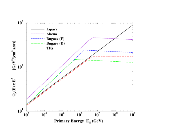
Figure 1: Comparison of primary cosmic-ray energy spectra, as given by different parametrizations (see Table 2). The primary flux is multiplied by $E_{N}^{3}$, so that the structure at the knee can be better appreciated, and the different parametrizations compared.

3.2 Interaction and attenuation lengths

The nucleonic interaction length, $\lambda_{N}$, represents the mean free path of nucleons in the atmosphere (given in g/cm²). It is related to $\sigma_{in}^{\!N-air}$, the total inelastic cross section for collisions of nucleons $(N)$ with air nuclei, through the relation

$$\lambda_{N}(E)=\frac{A.m_{p}}{\sigma_{in}^{\!N-air}(E)}=\frac{24100}{\sigma_{in}^{\!N-air}(E)},$$ (12)

where we used the average atomic number for air nuclei $A$=14.5, $m_{p}$ is the proton mass and $\sigma_{in}^{\!N-air}$ must be given in $mb$. There are different parametrizations to the inelastic $N-$air cross section as a function of energy. Some authors considered it to be constant[9, 12]; others to be rising with energy: as a power-law[16], as a logarithmic dependence[7, 17], or as a log-squared dependence[18, 19].

The attenuation length, $\Lambda_{N}$, which governs the exponential decay of the nucleonic flux with increasing depth, see Eq. (3), represents the net effect in the interplay between interaction losses and regeneration of the number of nucleons in the cascade development, and is given by

$$\Lambda_{N}\>=\>\frac{\lambda_{N}}{\left(1-Z_{NN}(\gamma)\right)}.$$ (13)

The interaction length $\lambda_{N}$ dictates the losses and the nucleon-to-nucleon spectrum-weighted Z-moment $Z_{NN}(\gamma)$ accounts for the survival rate of nucleons. $Z_{NN}$ is calculated in analogy to Eq. (7), with the outgoing particles being the regenerated nucleons. Some authors use an approximately constant value[7, 12, 19], others adopt Feynman-scaling with a change in value at the knee energy[5, 18], while in Ref. [13] it is assumed the violation of Feynman-scaling.

The charm particle of type-$i$ may have an interaction length $\lambda_{i}$ in the atmosphere calculated analogously as for the nucleons, Eq. (12), substituting $\sigma_{in}^{\!N-air}$ by $\sigma_{in}^{\!i-air}$. As in the parametrization of the nucleonic inelastic cross section, we find authors adopting a charm cross section which is constant[20], or which increases with energy either as a power-law[21], or logarithmically[7].

3.3 Charm production spectrum-weighted moments

The key information for the evaluation of the prompt lepton flux is the behavior of the charm spectrum-weighted moments, given by a specific charm production model. Among these models, we select three different ones, to be compared in the present study.

QGSM:

Quark Gluon String Model, a semiempirical model of charm production based on the non-perturbative QCD calculation by Kaidalov and Piskunova[22], normalized to accelerator data, and applied to the prompt muon calculation by Volkova et al.[9].

The Z-moments are calculated numerically from Eq. (7), with

$$\frac{dW^{Ni}}{dx_{F}}=\frac{\sigma_{NA}^{\!i}}{\sigma_{in}^{\!N-air}}\>\frac{df_{i}}{dx_{F}},$$ (14)

where the particle production spectrum is parametrized by:

$$\frac{df_{i}}{dx_{F}} = \>\>\>\ \frac{1.08}{x_{F}}\>(1-x_{F})^{5}\>\>\>\mbox{{\rm for $D$ production}},$$ (15)

$$= \>\>\>\ 1.4\>(1-x_{F})^{0.4}\>\>\>\mbox{{\rm for $\Lambda_{c}$ production}}.$$

For the total inelastic cross section, $\sigma_{in}^{\!N-air}$, we used a parametrization with a $\log^{2}$ energy dependence[18]. Following Ref.[9], a mild $\log$ energy dependence is assumed for the inclusive cross section of charm production, $\sigma_{NA}^{\!i}$, and the production of $D_{s}$ is neglected. Figure 2 displays the curves of Z-moments for the different charm components.

RQPM:

Recombination Quark Parton Model, a phenomenological non-perturbative approach, taking into account the contribution of the intrinsic charm to the production process, in which a $c\bar{c}$ pair is coupled to more than one constituent of the projectile hadron, as described by Bugaev et al.[7, 17].

Supposing Feynman-scaling to hold (RQPM-FS), the charm production Z-moments are given simply by:

$$Z_{Ni}(\gamma)\>=\>Z_{\gamma}\>=\>\mbox{\rm constant},$$ (16)

with parameters for different particles shown in Table 3. Assuming the scaling violation (RQPM-SV), the parametrization turns out to be:

$$Z_{Ni}(\gamma)\>=\>Z_{\gamma}\>\left(\frac{E_{N}}{E_{\gamma}}\right)^{\xi},$$ (17)

where $\xi=\>0.177-0.05\,\gamma$. The parameters are also given in Table 3. We obtained the all-charged $D$-meson Z-moment ($i=D^{\pm}$) by averaging the individual conjugate moments, the same being done for neutral $D$-mesons, ($i=D^{o},\bar{D}^{o}$). Ref.[7] does not take into account the contribution of $D_{s}$ mesons. A comparison of the resulting Z-moments, with and without scaling, is provided in Figure 3.

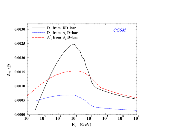
Figure 2: Charm Z-moment components for QGSM, as a function of energy.

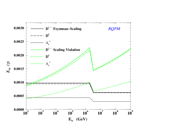
Figure 3: Charm Z-moment components for RQPM, considering respectively Feynman-scaling (FS) and scaling violation (SV), as a function of the energy.

Table 3: RQPM Z-moment parameters $Z_{\gamma}$ ⁽¹⁾.

Label	$\gamma$	$\xi$	$E_{\gamma}$ (GeV)	$Z_{\gamma}(D^{\pm})$	$Z_{\gamma}(D^{o},\bar{D}^{o})$	$Z_{\gamma}(\Lambda_{c}^{+})$
RQPM-FS	1.62	-	-	4.88 $\times 10^{-4}$	4.73 $\times 10^{-4}$	4.36 $\times 10^{-4}$
	2.02	-	-	3.14 $\times 10^{-4}$	3.09 $\times 10^{-4}$	2.95 $\times 10^{-4}$
RQPM-SV	1.62	0.096	$10^{3}$	5.55 $\times 10^{-4}$	5.35 $\times 10^{-4}$	4.9 $\times 10^{-4}$
	2.02	0.076	$10^{6}$	6.65 $\times 10^{-4}$	6.55 $\times 10^{-4}$	6.2 $\times 10^{-4}$
(1) According to Eqs. (16) and (17).

pQCD:

Perturbative QCD, as calculated by TIG[13], using the Monte Carlo program PYTHIA[23], explicitly evaluating the charm production, up to leading order (LO) in the coupling constant and including the next-to-leading order (NLO) distribution effects as an overall factor.

Figure 4 presents the curves for pQCD calculations of the charm production Z-moments carried out supposing a primary spectrum either with, or without, the knee. The values of Z-moments for $D$-mesons were extracted directly from Ref.[13]. The Z-moments for $\Lambda_{c}^{+}$ and $D_{s}$ are derived by taking $Z(\Lambda_{c})\simeq\>0.3\>Z(D)$ and $Z(D_{s})\simeq\>0.2\>Z(D)$, respectively, based on values assumed for the corresponding cross section ratios.

More recently Gelmini, Gondolo and Varieschi (GGV)[24] updated the calculation to include the full contribution of NLO predictions to the lepton fluxes. While TIG scales the LO cross sections by a constant factor of $K=2$ to obtain the NLO contribution, GGV evaluates explicitly the NLO component, as tailored by Mangano, Nason and Ridolfi[25]. At the end, the net calculation corresponds as to multiply the LO term by an energy dependent factor $K$. In the $10^{2}$ to $10^{11}$ GeV energy interval, it starts at the lowest energies with $K=3$, decreases to around 2 for most of the intermediate energies, increasing slightly at the high energy extreme. However, the main difference between the two calculations comes from the extrapolation of the gluon parton distribution function, which produces higher charm cross sections even at LO. We do not duplicate here the particular effects implied over the Z-moments, leaving to consider the overall changes, resulting from GGV approach, at the evaluation of the lepton fluxes. Despite these differences, the atmospheric cascading routines are the same in both TIG and GGV calculations. A discussion of an alternative evaluation of the charm production based on pQCD, compared to TIG’s calculation, is presented by Pasquali et al.[14].

In Section 4 we compare the resulting prompt lepton fluxes, evaluated using each of these models. It is interesting to include in this comparison the results obtained by E. Zas et al.[10]. They calculate extreme cases of charm production, at both low and high production rate limits. As for the high end, they assume a charm production cross section which is 10% of the total inelastic cross section (called Model-A), behaving as $\log^{2}(s)$ at high energies, $\sqrt{s}$ being the center-of-mass system (c.m.s.) energy. At the low end lies a pQCD model at NLO, with structure functions given by Kwiecinski-Martin-Roberts-Stirling[26], adopting one choice of parameters that leads to relatively hard parton distribution functions (called Model-E).

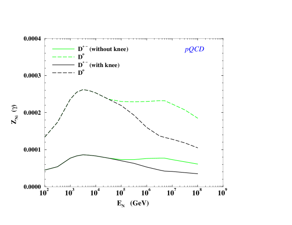
Figure 4: Charm Z-moment components for pQCD, considering the primary spectrum either with or without a knee, as a function of energy.

4 Results

4.1 High-energy atmospheric muon flux

A reproduction of calculated fluxes of high-energy muons reported by different authors is presented in Figure 5. Comparing the conventional flux, from the decay of pions and kaons, obtained by Lipari and TIG, with the prompt flux, calculated by Volkova et al., Bugaev et al., TIG, GGV and Zas et al., we note that the cross-over of the conventional and prompt components may occur at energies between $2\times 10^{3}$ GeV and $2\times 10^{6}$ GeV. The prompt flux intensity, itself, spans up to four orders of magnitude!

We remark that the lowest curves, labeled TIG, GGV and Zas (E), are calculated assuming the pQCD charm production model. Although based on the same framework, these calculations of the charm cross section are subjected to theoretical uncertainties, which arises from the possible range of charm quark masses, as well as the factorization and renormalization scale dependence. Moreover, different assumptions are made for the parton distribution functions, needed at very small parton momentum fractions, not measured at accelerators. The curve labeled Bugaev is calculated within the RQPM. As an intrinsic-charm model, it predicts relatively hard inclusive spectra. In spite of that, the total inclusive cross section can be made rather large, since it depends strongly on the assumptions about the charm structure function of the projectile hadron. The curve labeled Volkova is obtained from a parametrization given in Ref.[7], because the original work[9] quotes only flux ratios. The QGSM assumed in this calculation is considered to represent quite well open-charm production, and it is known to describe a wide variety of data on hadronic interactions. However, the model predicts a preferential production of certain secondary particle species which is not supported by experiment. In addition, predictions based on this model seem to exceed the experimental observations of horizontal air showers, measured by AKENO[27]. Finally, the calculation labeled Zas (A) represents an extreme and crude upper bound for the prompt fluxes, based on the assumption that a charm is produced $10\%$ of the time in these high-energy interactions. Actually, it is ruled out by the bounds set to the charm cross section from the above mentioned analysis of AKENO data.

One must be careful when analyzing differences in the curves of Figure 5. We call attention to the fact that not only different charm models are being compared. The reported prompt fluxes are calculated adopting different atmospheric cascading routines. In order to better evaluate the observed discrepancies, we proceed the analysis by taking into account the separate effect of each single ingredient in the shower process. Later on, we analyze the effect of multiple ingredients, to evaluate how the choice of a different combination may affect the final result.

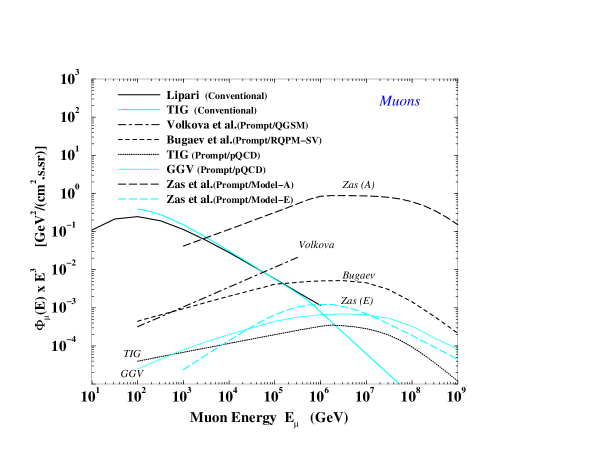
Figure 5: Comparison of calculated differential vertical muon fluxes at sea level, as reported by several authors. The fluxes are multiplied by $E_{\mu}^{3}$.

4.2 Single ingredient effects

If we calculate the fluxes of prompt neutrinos ($\nu_{\mu}$ and $\nu_{e}$), we obtain essentially the same values as the prompt muon flux (see for example Refs. [7, 13, 24]). The reason is that both the parent ($D$ or $\Lambda_{c}$) and the daughter ($K$ or $\Lambda_{o}$) particles are massive compared to the leptons and the decay kinematics become blind to lepton family number or flavor.

The prompt lepton flux is also essentially independent of $x$ (for depths greater than a few interaction lengths), due to the fact that the main contribution to the high-energy lepton flux must come from the first interactions of primary nucleons with air nuclei, while they are still energetic enough. In addition, for a fixed detection level, the flux is insensitive to the zenith angle $\theta$, up to the charm critical energy. This is also a consequence of the fact that the bulk of energetic leptons are produced high in the atmosphere and will reach the detector, regardless the amount of atmosphere traversed (less depth in the vertical direction, larger slant depths for showers close to the horizon). For energies above the critical energy, the charm particle decay length becomes comparable to the interaction length, and we feel the effects of its angular dependence, given in Eq. (10).

Since the prompt lepton flux is almost independent of lepton flavor, detection depth and zenith angle, hereafter we will perform our comparisons using the muon-neutrino vertical flux ($\theta=0^{o}$) at sea level ($x\approx 1000$ g/cm²).

First we investigate the effect of the primary spectrum at the top of the atmosphere (Section 3.1). To do so we calculate the prompt lepton flux, keeping all ingredients fixed, but the primary flux. Just for comparison purposes, we consider ingredients for the showering process used by Bugaev. The effect of the primary spectrum, alone, to the final result is considerable, as shown in Figure 6. The spread on the resulting fluxes generally increases with energy. For example, at $10^{9}$GeV, the difference between using Lipari’s single slope and TIG’s primary is a factor 10 times, while they started together at $10^{3}$ GeV. Also a big shift is present for the curve with AKENO primary against all others with knee, above $10^{5}$ GeV.

The next two ingredients considered are the nucleonic interaction length and the nucleonic Z-moment (Section 3.2). Apart from assuming a constant interaction length (as done by Lipari), for which the overestimated value at high energies pulls the neutrino flux down, the resulting fluxes are rather insensitive to the choice of $\lambda_{N}$. Similar situation occurs with the fluxes calculated changing only the nucleonic Z-moments, the difference being that the overestimated flux comes from TIG ($Z_{NN}(\gamma)\approx 0.5$, at energies below $10^{5}$ GeV), pushing the neutrino flux up, while other models ($Z_{NN}(\gamma)\approx 0.2-0.3$), result basically in the same final prompt flux.

The fluxes are also rather insensitive to the charm interaction length up to $10^{7}$ GeV, as they should, since that is about the value of $\varepsilon_{critic}$ for charmed particles (see Table 1). Above this range we discriminate the models up to a factor of two times, whether we use $\lambda_{i}$ constant or with a $\log(E)$ dependence.

When evaluating the effects of the choice of charm production model (Section 3.3), the big uncertainties in the inclusive cross sections of charm production are transmitted to the calculated prompt lepton fluxes, as seen in Figure 7. The spread between the prompt flux calculated with RQPM-SV and pQCD reaches a multiplicative factor of 20 at higher energies, solely due to the choice of $Z_{Ni}(\gamma)$.

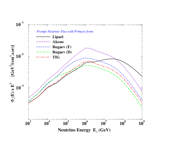
Figure 6: Comparison of prompt neutrino fluxes for different primary spectrum models (see Table 2), assuming all the other ingredients fixed.

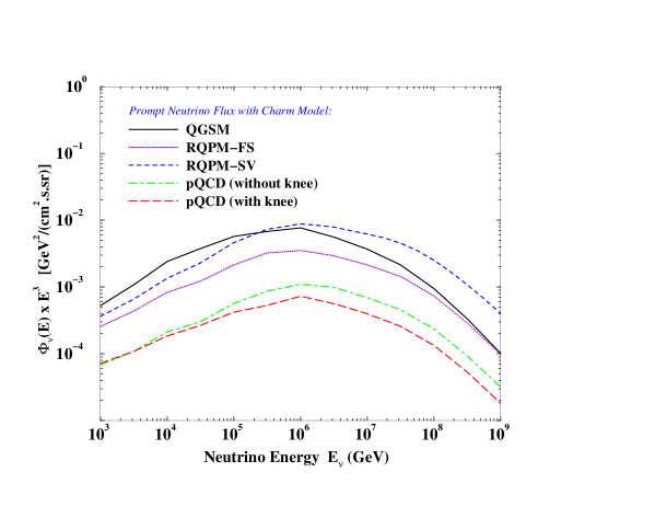
Figure 7: Comparison of prompt neutrino fluxes for different charm Z-Moment models (see Section 3.3), assuming all the other ingredients fixed.

4.3 Extreme ingredient combinations

In the previous section the effect of each individual ingredient of the atmospheric showering process has been appreciated. Now, we investigate how the choice of multiple ingredients combined in different ways affects the resulting flux. Let’s consider an example. The choice of the production model QGSM makes the flux dominates over other choices of charm production only up to about $2\times 10^{5}$ GeV, if all other parameters are fixed (Figure 7). The combination of the QGSM with the AKENO primary flux, which solely contributes to larger prompt flux up to $10^{7}$ GeV (Figure 6), makes this new set dominate upon a broader range of energy. Choosing a charm interaction length model that is responsible for increasing the prompt flux at higher energies, we build a set which dominates over yet a larger range. Such a combination of showering parameters leads to a maximum flux configuration. With a similar procedure we can build a minimum configuration. In this case it is interesting to consider the effect of Lipari’s primary up to the energy of the knee, above which Bugaev’s Model-D for the primary spectrum produces the minimum prompt flux. The other showering parameters may also be chosen as to stress the maximum or minimum possible behavior of a given flux calculation. Table 4 presents our suggestion of multiple ingredient combinations selected to obtain extreme outputs. The prompt lepton flux curve calculated for each charm production model (QGSM, RQPM or pQCD), can be shifted up or down, depending on the chosen combination of ingredients, an effect illustrated in Figures 8 to 10. The band in each figure reflects the freedom to change the resulting flux between the maximum (MAX) and minimum (MIN) extreme combinations listed in Table 4.

Table 4: Extreme ingredient combinations of atmospheric showering parameters, selected to obtain maximum or minimum behavior of prompt flux.

Ingredient	MAXIMUM Set	MINIMUM Set
$N_{0},\gamma$ (for $E<E_{knee}$)	AKENO	Lipari
$N_{0},\gamma$ (for $E>E_{knee}$)	AKENO	Bugaev-D
$\lambda_{N}(E)$	power-law[16]	constant[12]
$Z_{NN}(\gamma)$	scaling violation[13]	constant with knee[18]
$\lambda_{i}(E)$	constant[20]	$\log(E)$[7]

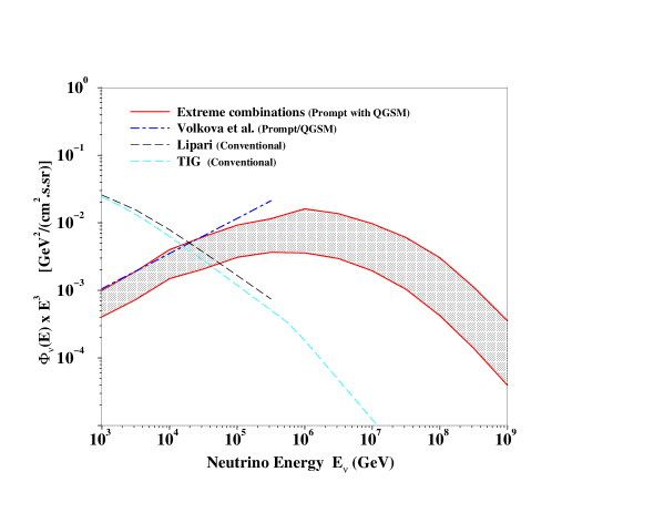
Figure 8: Prompt neutrino flux calculated with QGSM. The band represents the range between extreme ingredient combinations. Prompt flux from Volkova et al. and conventional neutrino fluxes also shown for illustration.

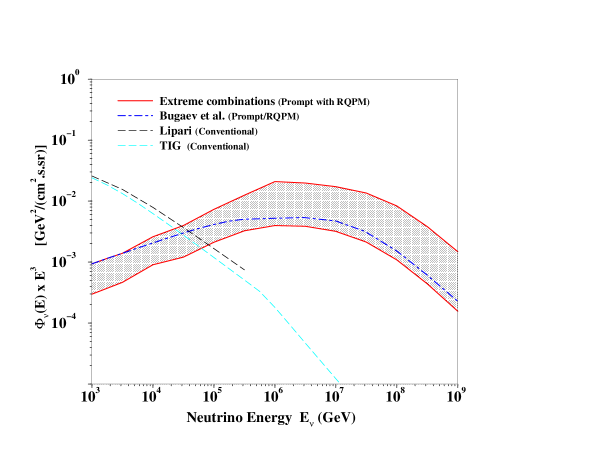
Figure 9: Prompt neutrino flux calculated with RQPM. The band represents the range between extreme ingredient combinations. Prompt flux from Bugaev et al. and conventional neutrino fluxes also shown for illustration.

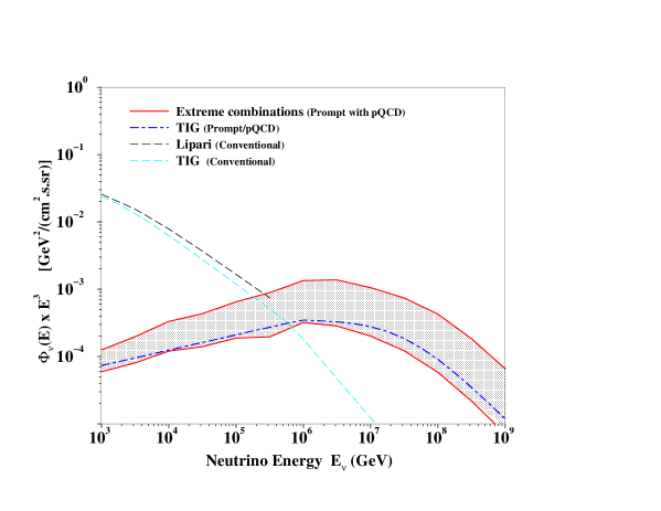
Figure 10: Prompt neutrino flux calculated with pQCD. The band represents the range between extreme ingredient combinations. Prompt flux from TIG and conventional neutrino fluxes also shown for illustration.

5 Conclusion

The calculation of the prompt lepton flux produced in the atmosphere by the semileptonic decay of charmed particles is rather straightforward, but we cannot say the same for the analysis of the results. For instance, the lack of precise information on high-energy charm inclusive cross-section in hadron-nucleus collisions is accompanied by a variety of options for the particle showering process in the atmosphere. We described different ingredients of the calculation, comparing side by side several parametrizations for each one of them, and evaluated their relative importance to the final result. The major effects are due to the choice of the primary spectrum at the top of the atmosphere and, of course, to the choice of the charm particle production model. Only first nucleonic interactions play essential role in determining the prompt lepton flux down at sea level, therefore variations in the nucleonic attenuation lengths are not that relevant, while the charm interaction length have some influence, above the charm particle critical energy. We observed how different combinations of ingredients can shift the resulting flux curves up or down. Therefore, the comparison between different calculations must be carried out with great care. The bands displayed in Figures 8-10 correspond to the allowed regions for the prompt lepton flux calculated respectively with the charm production models QGSM, RQPM and pQCD, if the showering process parameters are mixed differently.

The prompt lepton crossover energy, that is the energy above which the charm particle decay products dominate over the conventional pion and kaon decay induced fluxes, is yet an uncertain quantity. According to Figures 8-10, it may be anywhere between $10^{4}$ and $10^{6}$ GeV. If the cross-over is “low enough” (about $10^{4}$ GeV), then neutrino telescopes now operational can therefore take advantage of the isotropy of the prompt lepton flux, to search for an zenith angle independent component in their data. This can also be pursued by the analysis of the more copiously detected down-going muons.

Exploiting the case of tau-neutrinos, which may produce a clear signature in high-energy neutrino detectors[28], will be addressed in a future analysis. There is also the need for a more comprehensive description of the available data on charm production cross section, and its extrapolation to higher energies.

The prompt lepton flux is on the order-of-the-day of operating high-energy neutrino telescopes, because of the background it represents. Proposed experiments, like IceCube [29], may turn the arguments the other way around, for their measurements with enhanced sensitivity may provide outstanding information on heavy quark interactions, just by discriminating atmospheric from cosmic neutrinos, at energies above tens of TeV.

References

- [1] T.K. Gaisser, F. Halzen and T. Stanev, Phys. Rep. 258, 173 (1995); F. Halzen, Phys. Rep. 333-334, 349 (2000).
- [2] E. Andres et al. (The AMANDA Collaboration), Astropart. Phys. 13, 1 (2000).
- [3] V.A. Balkanov et al. (The BAIKAL Collaboration), Astropart. Phys. 14, 61 (2000).
- [4] C. Spiering, “Future High Energy Telescopes”, to appear in the Proceedings of the 19th International Conference On Neutrino Physics And Astrophysics - Neutrino 2000, June 16-21, 2000, Sudbury (Canada).
- [5] T.K. Gaisser, Cosmic Rays and Particle Physics, (Cambridge University, Cambridge, 1992).
- [6] D.E. Groom et al. (Particle Data Group), Eur. Phys. Jour. C15, 1 (2000).
- [7] E.V. Bugaev, A. Misaki, V.A. Naumov, T.S. Sinegovskaya, S.I. Sinegovsky and N. Takahashi, Phys. Rev. D 58, 054001 (1998).
- [8] L. Pasquali and M.H. Reno, Phys. Rev. D 59, 093003 (1999).
- [9] L.V. Volkova, W. Fulgione, P. Galeotti and O. Saavedra, Nuovo Cimento C 10, 465 (1987).
- [10] E. Zas, F. Halzen and R.A. Vázquez, Astropart. Phys. 1, 297 (1993).
- [11] R. Hagedorn, in Relativistic Kinematics, (Benjamin, NY, 1963).
- [12] P. Lipari, Astropart. Phys.1, 195 (1993).
- [13] M. Thunman, G. Ingelman and P. Gondolo, Astropart. Phys. 5, 309 (1996).
- [14] L. Pasquali, M.H. Reno and I. Sarcevic, Phys. Rev. D 59, 034020 (1999).
- [15] T.H. Burnett et al. (The JACEE Collaboration), in Proceedings of the 21st International Cosmic Ray Conference, Adelaide, Australia, Vol.3, p. 101 (1990).
- [16] T. Hara et al., in Proceedings of the 18th International Cosmic Ray Conference, Bangalore, India, Vol.9, p. 198 (1983); M. Nagano et al., J.Phys. G 10, 1295 (1984).
- [17] E.V. Bugaev, V.A. Naumov, S.I. Sinegovsky and E.S. Zaslavskaya, Nuovo Cimento C 12, 41 (1989).
- [18] C.G.S. Costa, F. Halzen and C. Salles, Phys. Rev. D 52, 3890 (1995); Phys. Rev. D 54, 5558 (1996).
- [19] M.M. Block, F. Halzen and T. Stanev, Phys. Rev. Lett. 83, 4926 (1999); Phys. Rev. D 62, 077501 (2000).
- [20] L.V. Volkova, Nuovo Cimento C 8, 552 (1985); Y. Minorikawa and K. Mitsui, Lett. Nuovo Cimento 44, 651 (1985).
- [21] K. Mitsui, Y. Minorikawa and H. Komori, Nuovo Cimento C 9, 995 (1986).
- [22] See, e.g. A.B. Kaidalov and O.I. Piskunova, Z. Phys. C 30, 145 (1986) and references therein.
- [23] T. Sjostrand, Comput. Phys. Commun. 82, 74 (1994).
- [24] G. Gelmini, P. Gondolo and G. Varieschi, Phys. Rev. D 61, 036005 (2000); Phys. Rev. D 61, 056011 (2000).
- [25] M.L. Mangano, P. Nason and G. Ridolfi, Nucl. Phys. B373, 295 (1992); Nucl. Phys. B405, 507 (1993).
- [26] See, e.g. A.D. Martin, W.J. Stirling and R.G. Roberts, Phys. Rev. D 47, 867 (1993).
- [27] M.C. Gonzales-Garcia, F. Halzen, R.A. Vázquez and E. Zas, Phys. Rev. D 49, 2310 (1994).
- [28] J.G. Learned and S. Pakvasa, Astropart. Phys.3, 267 (1995).
- [29] See, e.g. “The IceCube National Science Foundation Proposal,” available at the URL http://pheno.physics.wisc.edu/IceCube/ and also: F. Halzen et al., “From the first neutrino telescope, the Antartic Muon and Neutrino Detector Array AMANDA, to the IceCube Observatory”, in Proceedings of the 26th International Cosmic Ray Conference, South Lake City (USA), edited by D. Kieda, M. Salamon and B. Dingus, Vol. 2, 428-431 (1999).