Abstract

We study the virtual Compton amplitude in the generalized Bjorken region ($q^{2}\rightarrow\infty$, $t$ small) in QCD by means of a light–cone expansion of the product of e.m. currents in string operators in coordinate space. Electromagnetic gauge invariance (transversality) is maintained by including in addition to the twist–2 operators “kinematical” twist–3 operators which appear as total derivatives of twist–2 operators. The non-forward matrix elements of the elementary twist–2 operators are parametrized in terms of two-variable spectral functions (double distributions), from which twist–2 and 3 skewed distributions are obtained through reduction formulas. Our approach is equivalent to a Wandzura–Wilczek–type approximation for the twist–3 skewed distributions. The resulting Compton amplitude is manifestly transverse up to terms of order $t/q^{2}$. We find that in this approximation the tensor amplitude for longitudinal polarization of the virtual photon is finite, while the one for transverse polarization contains a divergence already at tree level. However, this divergence has zero projection on the polarization vector of the final photon, so that the physical helicity amplitudes are finite.

 
¹ E-mail: radyush@jlab.org . Also at Laboratory of Theoretical Physics, JINR, Dubna, Russia.
² E-mail: weiss@tp2.ruhr-uni-bochum.de

Contents

toc

I Introduction

Deeply virtual Compton scattering (DVCS) is currently receiving a lot of attention, as an exclusive process closely related to inclusive deep–inelastic scattering (DIS) [1, 2, 3]. The theory of DIS is well understood and can be formulated both in the field–theoretical framework of QCD or the particle–based language of the parton model. The relevant information about the non-perturbative structure of the nucleon is contained in expectation values of QCD light–ray operators in the nucleon, which can be interpreted as the parton distributions. Similarly, the DVCS amplitude in the asymptotic region can be expressed through off–diagonal (non-forward) matrix elements of light–ray operators, which also possess a partonic interpretation in terms of so-called “skewed” parton distributions (SPD’s). The initial motivation for considering DVCS was the hope that by measuring the SPD’s one could obtain information about the angular momentum distributions of quarks and gluons in the nucleon [1]. However, it was soon realized that the DVCS process is of interest in itself, independently of its connection to the nucleon spin problem. It is the simplest representative of a whole class of exclusive electroproduction processes, including also hard meson production, for which factorization can be proven in QCD at leading twist level [2, 3]. The first experimental observations of DVCS have recently been reported by the ZEUS [4], H1 [5], and HERMES [6] collaborations, and an extensive experimental program is planned at JLAB [7]. The DVCS process is also related, by crossing relations [8, 9], to the electroproduction of pairs of hadrons off a real photon, such as $\gamma^{*}\gamma\rightarrow 2\pi$ [10], which can be studied at $e^{+}e^{-}$ colliders.

The virtual Compton amplitude in the asymptotic region of large virtuality of the incoming photon, $-q_{1}^{2}\rightarrow\infty$, and small momentum transfer squared, $t\ll 1\,{\rm GeV}^{2}$, has been studied in QCD using expansion techniques familiar from DIS: The collinear expansion in momentum space [11], and the non-local light–cone expansion in coordinate space [12, 13]. Originally only the contribution from twist–2 operators was included in the calculation of the tensor amplitude [1, 3]. This approximation does not include subleading terms proportional to the transverse part of the momentum transfer, $r_{\perp}\equiv\Delta$, and the tensor amplitude thus obtained formally violates electromagnetic gauge invariance (transversality) by terms linear in $\Delta$. To remedy this, Guichon and Vanderhaeghen [15] proposed to add a term linear in $\Delta$, producing a tensor amplitude which is transverse up to terms of order $\Delta^{2}\sim t$. It is clear that in a QCD treatment such a term could come only from contributions of operators of higher twist ($>2$). Indeed, calculations by various groups [16, 17, 18, 19] have recently shown that the term introduced in Ref.[15] appears naturally as part of the twist–3 contribution to the Compton amplitude. Anikin et al. [16], applying the momentum–space collinear expansion up to twist–3 level, reproduced not only the “improved” twist–2 structure of Ref.[15], but found also other, separately transverse twist–3 structures in the tensor amplitude, which can contribute to the observables of the DVCS process. A similar result was obtained by Penttinen et al. [17], who computed the DVCS amplitude to accuracy $1/\sqrt{-q_{1}^{2}}$ in a parton model approach. Within the framework of the coordinate–space light–cone expansion the twist–3 contribution to the DVCS amplitude was studied by Belitsky and Müller [18]. In particular, these authors demonstrated that in order to get a gauge invariant result up to terms of order $t/q_{1}^{2}$ it is sufficient to retain only a certain part of the full twist–3 SPD’s which is obtained by Wandzura–Wilczek–type relations from the twist–2 distributions. Kivel et al. [20] noted that the Wandzura–Wilczek expression for the tensor amplitude contains a divergence in the part corresponding to transverse polarization of the virtual photon.

In this paper we address the question of transversality of the DVCS amplitude within the framework of the light–cone expansion of the current product in QCD string operators in coordinate space developed by Balitsky and Braun [13]. (A short summary of our results has already been given in Ref.[19].) The investigation consists of two main parts. First, we show that transversality of the light–cone expansion can be achieved, in the minimal sense, by including in the expansion certain operators which are algebraically of twist 3 but given by total derivatives of twist–2 string operators. We shall refer to these as “kinematical” twist–3 contributions, in order to distinguish them from the twist–3 contributions involving quark–gluon operators which cannot be reduced to total derivatives by the equations of motion. The operations necessary to include the “kinematical” twist–3 contributions in the light–cone expansion can be performed using the calculus of QCD string operators. The result has the same form as the usual twist–2 part of expansion, but with certain finite translations of the center coordinates of the twist–2 string operators (similar expressions were derived independently in Refs.[18, 20]).

Second, we investigate whether the approximation of keeping only the “kinematical” twist–3 contributions required by transversality leads to useful results at the level of the hadronic DVCS amplitude. To this end, we parametrize the matrix elements of the fundamental twist–2 operators in terms of two–variable spectral functions (double distributions) [3, 21, 22, 9]. The Compton amplitude in the DVCS limit, including the “kinematical” twist–3 contributions, can be expressed in terms a number of one-variable skewed distributions (SPD’s), which are obtained in the form of one–dimensional reductions of the twist–2 double distribution. The resulting tensor amplitude is manifestly transverse up to terms of order $t/q_{1}^{2}$ or $m^{2}/q_{1}^{2}$ ($m$ is the target mass), i.e., its contraction with the four–momentum of the initial photon, $q_{1\mu}T_{\mu\nu}$, and that of the final photon, $T_{\mu\nu}q_{2\nu}$, are both of order $t/q_{1}^{2}$ or $m^{2}/q_{1}^{2}$. We find that our approximation gives a finite result for the part of the tensor amplitude corresponding to longitudinal polarization of the initial photon, while the part corresponding to transverse polarization contains a divergence. However, as we shall show, the divergent part has zero projection on the polarization vector of the final (real) photon, so it does not affect the physical helicity amplitudes.

Our approach of keeping only the “kinematical” twist–3 operators in the coordinate–space light cone expansion is actually equivalent to the Wandzura–Wilczek–type approximation for the twist–3 SPD’s introduced in Ref. [18]. In addition to giving an alternative derivation of this approximation, an important advantage of our treatment is the possibility to incorporate the formalism of double distributions [3, 21, 22, 9]. The twist–2 as well as the new twist–3 SPD’s are obtained by reduction formulas from the fundamental twist–2 double distribution. This allows for a straightforward derivation of the properties of these new functions and the Wandzura–Wilczek–type relations between them. In particular, the fact that this approximation gives finite results for the tensor amplitude for longitudinally polarized initial photon, but contains a divergence in the case of transverse polarization (which, however, drops out of the physical helicity amplitudes), can immediately be understood on the basis of the reduction formulas.

The plan of this paper is as follows. Section II gives a brief summary of the kinematics of virtual Compton scattering in the generalized Bjorken limit. In Section III we discuss the peculiarities of the light–cone expansion in the “non-forward” case, where total derivative operators contribute. Our treatment is based on the formalism developed by Balitsky and Braun [13]. In Section III A we recall the main steps in the twist decomposition of string operators. In Section III B we investigate the problem of transversality of the light–cone expansion at operator level in coordinate space. We observe that the twist–2 contribution is not transverse, and show that transversality can be restored by including total derivatives of twist–2 operators, which are algebraically of twist 3. We first formulate this as as an iterative procedure generating an infinite series of total derivatives of twist–2 operators, then show that this series can be summed up in closed form to give finite translation operators acting on the twist–2 string operators (details are given in Appendix A). A manifestly transverse expression for the light–cone expansion of the current product in terms of twist–2 operators and their total translations is presented. In Section IV we use our result for the light–cone expansion including “kinematical” twist–3 terms to compute the hadronic DVCS amplitude. For simplicity we consider the case of a pion target, which has spin 0 and definite $C$–parity. In Section IV A we describe the spectral representation of the fundamental twist–2 matrix elements in terms of double distributions. The matrix elements of the vector–type string operators including the “kinematical” twist–3 terms are then derived in Section IV B. The new SPD’s are introduced through reduction formulas, and their properties are discussed. The DVCS amplitude for the pion is computed in Section IV C. We inspect the singular integrals resulting from the inclusion of the “kinematical” twist–3 terms. We show that the tensor amplitude for transverse polarization of the initial (virtual) photon contains a divergence, but that this divergence is “harmless” in the sense that it has zero projection on the polarization vector of the final photon. In Section IV D we reformulate our results for the matrix elements and the Compton amplitude, introducing a new SPD as a Wandzura–Wilczek–type transformation of the basic twist–2 SPD. This allows us to demonstrate that our approach is equivalent to the Wandzura–Wilczek approximation proposed in Ref.[18]. In this language, the singularity for transverse polarization described in Section IV C appears due to a discontinuity of the Wandzura–Wilczek–transformed SPD at $x=\xi$, which occurs independently of the dynamical behavior of the underlying twist–2 matrix elements. Our conclusions are summarized in Section V.

In this paper we study the properties of the DVCS amplitude including “kinematical” twist–3 contributions at tree level. We shall not be concerned with logarithmic corrections resulting from the scale dependence of the operators (the evolution of the skewed distributions). For the twist–2 operators this problem has exhaustively been treated in the literature, see e.g. Refs.[1, 3, 23, 24, 25, 26, 27]. The generalization of the evolution equations to the “kinematical” twist–3 contribution discussed in the present paper is in principle straightforward but will not be pursued here.

II Virtual Compton amplitude in the generalized Bjorken limit

Virtual Compton scattering. For a unified description of the kinematics of processes such as DIS and DVCS let us imagine a general virtual Compton scattering process off a hadron,

$$\gamma^{\ast}(q_{1})\;+\;h(p_{1})\;\rightarrow\;\gamma^{\ast}(q_{2})\;+\;h(p_{2}),$$ (1)

where the incoming photon has space–like virtuality, $q_{1}^{2}<0$, and the final photon may have any virtuality allowed by four–momentum conservation; in particular, we shall allow for the final photon to be real, $q_{2}^{2}=0$. It is convenient to use as independent momentum variables the average of the photon and hadron momenta, $q$ and $p$, and the momentum transfer, $r$:

$$p_{1,2}\;\;=\;\;p\pm\frac{r}{2},\hskip 50.00008ptq_{1,2}\;\;=\;\;q\mp\frac{r}{2}.$$ (2)

From the mass shell conditions, $p_{1}^{2}=p_{2}^{2}=m^{2}$, it follows that

$$(pr)\;\;=\;\;0,\hskip 50.00008ptp^{2}\;\;=\;\;m^{2}-\frac{t}{4},\hskip 50.00008ptt\;\;\equiv\;\;r^{2}.$$ (3)

In the following we shall neglect the target mass and put $m=0$.

The amplitude for the virtual Compton process is defined by the transition matrix element of the time–ordered product of two electromagnetic current operators between the hadronic states:

$$T_{\mu\nu}\;\;=\;\;i\int d^{4}z\;e^{i(qz)}\langle p-r/2|{\rm T}\,J_{\mu}(-z/2)J_{\nu}(z/2)|p+r/2\rangle.$$ (4)

This tensor is transverse with respect to the incoming and outgoing photon momenta:

$$\left(q-\frac{r}{2}\right)_{\mu}T_{\mu\nu}\;\;=\;\;0,\hskip 50.00008ptT_{\mu\nu}\left(q+\frac{r}{2}\right)_{\nu}\;\;=\;\;0,$$ (5)

which is an immediate consequence of current conservation, $\partial_{\mu}J_{\mu}(x)=0$. Separating the symmetric and antisymmetric tensor parts of $T_{\mu\nu}$ (with otherwise same arguments),

$$\left.\begin{array}[]{c}T_{\{\mu\nu\}}\\[6.45831pt] T_{[\mu\nu]}\end{array}\right\}\;\;\equiv\;\;\frac{1}{2}\left(T_{\mu\nu}\pm T_{\nu\mu}\right),$$ (6)

the two conditions Eq.(5) can also be stated in the form

$$q_{\mu}T_{\{\mu\nu\}} = \frac{r_{\mu}}{2}T_{[\mu\nu]},$$ (7)

$$q_{\mu}T_{[\mu\nu]} = {r_{\mu}\over 2}T_{\{\mu\nu\}}.$$ (8)

One notes that in the case of non-forward scattering, $r\neq 0$, the transversality conditions generally imply relations between the symmetric and antisymmetric parts of the amplitude. It is only in the limit of forward scattering, $r=0$, (as is relevant e.g. to deep–inelastic scattering) that the two transversality conditions decouple and turn into conditions on the symmetric and the antisymmetric parts separately.

Generalized Bjorken region: DIS and DVCS. We shall consider the amplitude for the virtual Compton process, Eq.(1), in two different asymptotic regions, both characterized by large virtuality of the incoming photon. One is the region corresponding to deep–inelastic scattering (DIS), where one is interested in the forward scattering amplitude ($q_{1}=q_{2}=q,p_{1}=p_{2}=p,r=0$) in the limit $q_{1}^{2}\rightarrow\infty,(p_{1}q_{1})\rightarrow\infty$, with $x_{B}\equiv-q_{1}^{2}/[2(p_{1}q_{1})]$ fixed. The other is the region of deeply virtual Compton scattering (DVCS), where one is dealing with the amplitude for production of a real photon, $q_{2}^{2}=0$, in the limit $q_{1}^{2}\rightarrow\infty,(p_{1}q_{1})\rightarrow\infty$, again with $x_{B}\equiv-q_{1}^{2}/[2(p_{1}q_{1})]$ fixed. This process requires a non-zero momentum transfer from the initial to the final hadron, ($p_{1}-p_{2}\equiv r\neq 0$), with $(rq_{1})\rightarrow\infty$ proportional to $q_{1}^{2}$. One considers a situation where $t\equiv r^{2}<0$ does not grow with $q_{1}^{2}$. In order to treat both asymptotic regions within a common framework it is convenient to introduce two scaling variables,

$$\xi\;\;\equiv\;\;\frac{-q^{2}}{2(pq)},\hskip 50.00008pt\eta\;\;\equiv\;\;\frac{(rq)}{2(pq)},$$ (9)

where $\eta$ is referred to as “skewedness”. The virtualities of the incoming and outgoing photon can then be expressed as

$$q_{1}^{2} = \left(1+\frac{\eta}{\xi}\right)q^{2}+\frac{t}{4},$$ (10)

$$q_{2}^{2} = \left(1-\frac{\eta}{\xi}\right)q^{2}+\frac{t}{4},$$ (11)

and the Bjorken variable becomes

$$x_{B}\;\;=\;\;\frac{-q_{1}^{2}}{2(p_{1}q_{1})}\;\;\equiv\;\;\frac{\xi+\eta}{1+\eta}.$$ (12)

Because of Eq.(10) we may generally use $q^{2}$ instead of $q_{1}^{2}$ as the large invariant. The two situations, DIS and DVCS, now correspond to

$$\begin{array}[]{rll}\mbox{DIS:}&\;\;\eta\;=\;0,&\;\;x_{B}\;=\;\xi,\\[8.61108pt] \mbox{DVCS:}&\;\;\eta\;=\;\xi,&\;\;x_{B}\;=\;\displaystyle{\frac{2\xi}{1+\xi}}.\end{array}$$ (13)

Aim of the present calculation. In this paper we calculate the virtual Compton amplitude, Eq.(4), in DVCS kinematics, neglecting contributions of order $t/q^{2}$ or $m^{2}/q^{2}$. Specifically, we aim to compute the tensor amplitude to an accuracy such that the transversality conditions, Eqs.(5) viz. (8), are satisfied up to terms of order $t/q^{2}$ or $m^{2}/q^{2}$. In this approximation the kinematical limits for $\xi$ are

$$0\leq\xi\leq 1,$$ (14)

which is equivalent to $0\leq x_{B}\leq 1$. For DVCS it is convenient to separate from the momentum transfer, $r$, the component parallel to $p$, which is responsible for producing the large scalar when contracting with $q$, i.e., to write

$$r\;\;=\;\;2\xi p\;+\;\Delta.$$ (15)

The remaining part of the momentum transfer, $\Delta$, satisfies $(\Delta q)=-t/4$ and $(\Delta p)=-\xi t/2$. Since $p$ is time-like and $q$ space-like, and since furthermore $\Delta$ itself is space–like, $\Delta^{2}=(1-\xi^{2})t<0$, it follows that all components of $\Delta$ must be of order $|t|^{1/2}$:

$$\Delta\;\;\propto\;\;|t|^{1/2}.$$ (16)

This means that when computing the DVCS amplitude using the light–cone expansion we may expand the ingredients — the momentum–space quark propagators and the hadronic matrix elements — in $\Delta$, since this four–vector cannot produce any large scalars even when contracted with the photon momentum, $q$. This would not be possible for the full momentum transfer, $r$, since $(rq)$ is not small. In the language of the parton model, the component $2\xi p$ of the momentum transfer would be identified with the longitudinal component, while $\Delta$ would be the transverse component, $r_{\perp}$. Note that in our approach the decomposition of the momentum transfer, Eq.(15), appears on purely kinematical grounds, without reference to a particular frame.

III Light–cone expansion in the non-forward case

A Twist decomposition of string operators: Twist 2

The behavior of the virtual Compton amplitude, Eq.(4), in the generalized Bjorken limit (DIS or DVCS) is dominated by the light–cone singularity of the time–ordered product of the two electromagnetic currents, which is a consequence of the asymptotic freedom of QCD. An asymptotic expansion of the Compton amplitude in inverse powers of $1/q^{2}$ can be derived from the light–cone expansion of the current product. In this section we discuss the peculiarities of the light–cone expansion in the “non-forward” case, i.e., finite momentum transfer in the matrix elements, as is relevant e.g. for DVCS. An additional complication compared to the “forward” case arises due to the fact that total derivatives of operators can contribute to the matrix elements, which greatly enlarges the set of operators participating in the expansion to a given accuracy. In particular, we show here that keeping the total derivatives of twist–2 operators (which are operators formally of twist 3) is essential for maintaining transversality of the leading term in the light–cone expansion. We shall proceed step by step. We first investigate the well–known twist–2 contribution and show that, in the non-forward case, it is not transverse to the accuracy required. We then formulate a procedure how transversality can be “repaired” by including total derivatives of twist–2 operators, order–by–order in the number of total derivatives. Finally, we show that the series of total derivatives of twist–2 operators can be summed up in closed form, resulting in an expression involving certain finite translations of the original twist–2 operators, which is manifestly transverse.

Expansion in string operators. We shall be concerned with the light–cone expansion of the current product,

$$\Pi_{\mu\nu}(x,y)\;\;\equiv\;\;i{\rm T}J_{\mu}(x)J_{\nu}(y),$$ (17)

where $J_{\mu}(x)$ is the vector current operator. It is convenient to introduce the center and relative coordinates of the two points, $x$ and $y$,

$$X\;\;=\;\;(x+y)/2,\hskip 50.00008ptz\;\;=\;\;y-x,\hskip 50.00008pt\left.\begin{array}[]{c}x\\ y\end{array}\right\}\;\;=\;\;X\mp z/2,$$ (18)

and to regard the current product as a function of these variables. The light–cone expansion is derived from a formal expansion of the current product in QCD string (non-local) operators in a background gauge field, which are subsequently decomposed in operators of definite twist. This expansion is generated by contracting the quark fields in Eq.(17) with the quark Green function in a background gauge field, and expanding in powers of insertions of the background field in the Fock–Schwinger gauge. The resulting expansion can be formulated in a gauge–invariant way by introducing QCD string operators with fields connected by gauge links. It is known that the leading light–cone singularity is contained in the contraction corresponding to the simplest two–point string operator (the “handbag” diagram):

$$\Pi_{\mu\nu}(z|X) \equiv i{\rm T}J_{\mu}(X-z/2)J_{\nu}(X+z/2)$$ (19)

$$= \bar{\psi}(X-z/2)\frac{\gamma_{\mu}\hat{z}\gamma_{\nu}}{2\pi^{2}z^{4}}[X-z/2,X+z/2]\psi(X+z/2)$$ (20)

$$+ (z\rightarrow-z,\mu\leftrightarrow\nu).$$ (21)

$$+ 1/z^{2},\ldots$$ terms (22)

Here

$$\frac{\hat{z}}{2\pi^{2}(z^{2}-i0)^{2}}\;\;=\;\;\int\frac{d^{4}k}{(2\pi)^{4}}e^{-i(kz)}\frac{\hat{k}}{k^{2}+i0},\hskip 50.00008pt\hat{z}\;\;\equiv\;\;z_{\mu}\gamma_{\mu}\;\;\;\mbox{\it etc.},$$ (23)

is the free quark propagator in coordinate representation. Reducing the product of three gamma matrices, Eq.(22) can be written as

$$\Pi_{\mu\nu}(z|X)$$ (24)

$$= \frac{2z_{\rho}}{\pi^{2}z^{4}}\left\{\phantom{-i}s_{\mu\rho\nu\sigma}\left[\bar{\psi}(X-z/2)\gamma_{\sigma}[X-z/2,X+z/2]\psi(X+z/2)\;-\;(z\rightarrow-z)\right]\phantom{\frac{2z_{\rho}}{\pi^{2}z^{4}}}\right.$$ (26)

$$\left.\phantom{\frac{z_{\rho}}{2\pi^{2}z^{4}}}-i\epsilon_{\mu\rho\nu\sigma}\left[\bar{\psi}(X-z/2)\gamma_{\sigma}\gamma_{5}[X-z/2,X+z/2]\psi(X+z/2)\;+\;(z\rightarrow-z)\right]\right\},$$

where

$$s_{\mu\rho\nu\sigma}\;\;=\;\;\frac{1}{4}{\rm tr}\left[\gamma_{\mu}\gamma_{\rho}\gamma_{\nu}\gamma_{\sigma}\right]\\ \;\;=\;\;g_{\mu\rho}g_{\nu\sigma}-g_{\mu\nu}g_{\rho\sigma}+g_{\mu\sigma}g_{\nu\rho}.$$ (27)

In the string operators in Eq.(22) and (26) the gauge link runs along the straight line connecting the two space–time points:

$$[x,y]\;\;\equiv\;\;{\rm P}\exp i\int_{0}^{1}du\;(x-y)_{\alpha}A_{\alpha}(ux+\bar{u}y),\hskip 50.00008pt\bar{u}\equiv 1-u.$$ (28)

For brevity we shall in the following not write the links between the fields; it will always be understood that the fields in the string operator (including possible insertions of gauge fields at intermediate points) are connected by gauge links along the straight line.

Differentiating string operators. For a given background gauge field the link operator defined by Eq.(28) is a uniquely defined function of the end points. In particular, when differentiating the string operator with respect to its end points one is changing the contour of integration by an infinitesimal amount, so the link operator gets differentiated as well. There are generally two contributions from differentiating the link operators. One gives the gauge potentials at the end points, which combine with the derivatives acting on the quark fields to give covariant derivatives. The other can be expressed as a line integral of the gauge field along the contour of the string. For the derivative of the string operators in Eq.(26) with respect to the relative coordinate we find:

$$\frac{\partial}{\partial z_{\mu}}\bar{\psi}(X-z/2)\gamma_{\sigma}\psi(X+z/2)$$ (29)

$$= \frac{1}{2}\,\bar{\psi}(X-z/2)\left(\stackrel{{\scriptstyle\leftarrow}}{{\nabla}}_{\mu}\gamma_{\sigma}\;+\;\gamma_{\sigma}\stackrel{{\scriptstyle\rightarrow}}{{\nabla}}_{\mu}\right)\psi(X+z/2)$$ (30)

$$- i\int_{-1}^{1}dt\,t\;\bar{\psi}(X-z/2)\gamma_{\sigma}z_{\alpha}F_{\mu\alpha}(X+tz/2)\psi(X+z/2),$$ (31)

where gauge links between the fields are implicit everywhere; for the string operator with Dirac matrix $\gamma_{\sigma}\gamma_{5}$ one should replace $\gamma_{\sigma}\rightarrow\gamma_{\sigma}\gamma_{5}$ everywhere. The derivative with respect to the center coordinate (we refer to it as “total” derivative) takes the form

$$\frac{\partial}{\partial X_{\mu}}\bar{\psi}(X-z/2)\gamma_{\sigma}\psi(X+z/2)$$ (32)

$$= \bar{\psi}(X-z/2)\left(-\stackrel{{\scriptstyle\leftarrow}}{{\nabla}}_{\mu}\gamma_{\sigma}\;+\;\gamma_{\sigma}\stackrel{{\scriptstyle\rightarrow}}{{\nabla}}_{\mu}\right)\psi(X+z/2)$$ (33)

$$- 2i\int_{-1}^{1}dt\;\bar{\psi}(X-z/2)\gamma_{\sigma}z_{\alpha}F_{\mu\alpha}(X+tz/2)\psi(X+z/2).$$ (34)

Here

$$\stackrel{{\scriptstyle\rightarrow}}{{\nabla}}_{\mu}\psi(x) \equiv \phantom{-}\partial_{\mu}\psi(x)-iA_{\mu}(x)\psi(x),$$ (35)

$$\bar{\psi}(x)\stackrel{{\scriptstyle\leftarrow}}{{\nabla}}_{\mu} \equiv -\partial_{\mu}\bar{\psi}(x)-i\bar{\psi}(x)A_{\mu}(x)$$ (36)

are the right and left covariant derivatives, and

$$F_{\mu\alpha}\;\;\equiv\;\;i\left[\stackrel{{\scriptstyle\rightarrow}}{{\nabla}}_{\mu},\stackrel{{\scriptstyle\rightarrow}}{{\nabla}}_{\alpha}\right]$$ (37)

the field strength.

Twist–2 part of string operators. The string operators in Eq.(26) have as yet no definite twist. Consequently, the “handbag” contribution to the current product, Eq.(26), as it stands, contains also subleading contributions in $1/z^{2}$, which would be of the same order ($1/z^{2}$ or less singular) as contributions from quark–gluon string operators not included in Eq.(26). The leading $1/z^{4}$ singularity is given by the twist–2 part of the string operators. The latter is defined as those operators obtained by formally Taylor–expanding the string operators in Eq.(26) in the separation, $z$, and retaining only the totally symmetric traceless parts of the coefficients in the expansion:

$$\left[\bar{\psi}(X-z/2)\gamma_{\sigma}\psi(X+z/2)\right]^{\rm twist-2}$$ (38)

$$\equiv \sum_{n=0}^{\infty}\frac{1}{n!}\;z_{\alpha_{1}}\ldots z_{\alpha_{n}}\;\bar{\psi}(X)\left[\gamma_{\left\{\sigma\right.}\stackrel{{\scriptstyle\leftrightarrow}}{{\nabla}}{}_{\!\!\alpha_{1}}\ldots\stackrel{{\scriptstyle\leftrightarrow}}{{\nabla}}{}_{\!\!\left.\alpha_{n}\right\}}-\mbox{traces}\right]\psi(X),$$ (39)

and similarly for the operator with Dirac matrix $\gamma_{\sigma}\gamma_{5}$. Here $\stackrel{{\scriptstyle\leftrightarrow}}{{\nabla}}{}_{\!\!\equiv}(\stackrel{{\scriptstyle\rightarrow}}{{\nabla}}+\stackrel{{\scriptstyle\leftarrow}}{{\nabla}})/2$. As was shown in Ref.[13], the two operations, “symmetrization” and “subtraction of traces”, can in fact be carried out directly at the level of non-local operators, without having to go through the series of local operators [28]. The part of the string operator corresponding to totally symmetric local tensor operators is projected out by the operation

$$\left[\bar{\psi}(X-z/2)\gamma_{\sigma}\psi(X+z/2)\right]^{\rm sym}\;\;=\;\;\frac{\partial}{\partial z_{\sigma}}\int_{0}^{1}dt\;\bar{\psi}(X-tz/2)\hat{z}\psi(X+tz/2).$$ (40)

The subtraction of traces can be achieved by noting that the tracelessness of the local operators in the expansion, Eq.(39), implies that the string operator contracted with $z_{\sigma}$ should satisfy the d’Alembert equation with respect to $z$:

$$\Box_{z}\;\left[\bar{\psi}(X-z/2)\hat{z}\psi(X+z/2)\right]^{\rm traceless}\;\;=\;\;0.$$ (41)

Thus, combining the two operations, the twist–2 part of the vector string operator (for arbitrary $z^{2}\neq 0$) is obtained by substituting in the R.H.S. of Eq.(40) the solution of Eq.(41) with “initial conditions” given by the operator $\bar{\psi}(X-z/2)\hat{z}\psi(X+z/2)$ at $z^{2}=0$. On the light cone ($z^{2}=0$) trace subtraction is irrelevant, and the twist–2 part of the vector string operator coincides with the symmetric part as defined by Eq.(40).

When parametrizing the hadronic matrix elements of the operators, the $z^{2}$– (“trace”) terms in the matrix element are proportional to dimensionful scalars characterizing the target — the target mass, $m^{2}$, or the square of the momentum transfer, $t$. The inclusion of the $z^{2}$ terms in the calculation of the Compton amplitude then generates $m^{2}/q^{2}$– (target mass) and $t/q^{2}$–corrections to the DVCS amplitude. Here we shall neglect such corrections, so that the $z^{2}$–terms in the matrix elements need not be subtracted explicitly.

Twist–2 contribution to the light–cone expansion. The twist–2 part of the current product, which we denote by $\Pi_{\mu\nu}^{(0)}$, is given by Eq.(26), with the string operators replaced by their symmetric parts (we do not worry about trace subtraction):

$$\Pi_{\mu\nu}^{\rm(0)}(z|X) = \frac{2z_{\rho}}{\pi^{2}z^{4}}\left\{\phantom{-i}s_{\mu\rho\nu\sigma}\left[\bar{\psi}(X-z/2)\gamma_{\sigma}\psi(X+z/2)\phantom{\gamma_{5}}-(z\rightarrow-z)\right]^{\rm sym}\right.$$ (43)

$$\phantom{\frac{z_{\rho}}{2\pi^{2}z^{4}}}\left.-i\epsilon_{\mu\rho\nu\sigma}\left[\bar{\psi}(X-z/2)\gamma_{\sigma}\gamma_{5}\psi(X+z/2)+(z\rightarrow-z)\right]^{\rm sym}\right\}.$$

Using the property Eq.(41), and the fact that the coefficient function — the free fermion propagator, Eq.(23) — satisfies

$$\frac{\partial}{\partial z_{\rho}}\left(\frac{z_{\rho}}{2\pi^{2}z^{4}}\right)\;\;=\;\;-i\delta^{(4)}(z),$$ (44)

one can easily show that the twist–2 part of the current product satisfies

$$\frac{\partial}{\partial z_{\mu}}\Pi_{\{\mu\nu\}}^{(0)}\;\;=\;\;0,\hskip 50.00008pt\frac{\partial}{\partial z_{\mu}}\Pi_{[\mu\nu]}^{(0)}\;\;=\;\;0,$$ (45)

where

$$\left.\begin{array}[]{c}\Pi_{\{\mu\nu\}}^{(0)}\\[6.45831pt] \Pi_{[\mu\nu]}^{(0)}\end{array}\right\}\;\;\equiv\;\;\frac{1}{2}\left[\Pi_{\mu\nu}^{(0)}\pm\Pi_{\nu\mu}^{(0)}\right]$$ (46)

denote the Lorentz–tensor symmetric and antisymmetric parts. These properties play an important role in ensuring transversality of the light–cone expansion, as will be shown in the following subsection.

B Transversality and twist–3 operators

Transversality of the twist–2 contribution. We now turn to the question how to maintain transversality (electromagnetic gauge invariance) in the light–cone expansion of the current product. For the operator product, Eq.(17), regarded as a function of the two points, $x$ and $y$, current conservation implies that

$$\frac{\partial}{\partial x_{\mu}}\Pi_{\mu\nu}(x,y)\;\;=\;\;0,\hskip 56.9055pt\frac{\partial}{\partial y_{\nu}}\Pi_{\mu\nu}(x,y)\;\;=\;\;0.$$ (47)

In terms of the center and relative coordinates, Eq.(18), these conditions take the form

$$\frac{\partial}{\partial z_{\mu}}\Pi_{\{\mu\nu\}}(z|X) = \frac{1}{2}\frac{\partial}{\partial X_{\mu}}\Pi_{[\mu\nu]}(z|X),$$ (48)

$$\frac{\partial}{\partial z_{\mu}}\Pi_{[\mu\nu]}(z|X) = \frac{1}{2}\frac{\partial}{\partial X_{\mu}}\Pi_{\{\mu\nu\}}(z|X).$$ (49)

One sees that the transversality conditions relate the Lorentz–tensor symmetric and antisymmetric parts of the operator product; cf. Eq.(8) for the Compton amplitude.

In DIS the twist–2 part of the light–cone expansion, Eq.(43), gives the leading contribution to the structure functions at large $q^{2}$. In this case one is dealing with forward matrix elements of the twist–2 operators, so that all total derivatives of operators (i.e., derivatives $\partial/\partial X$) have zero matrix elements. The two conditions, Eqs.(48) and (49), decouple, and the properties Eq.(45) are sufficient to guarantee transversality of both the symmetric and antisymmetric parts separately. However, one immediately sees that in the case of non-forward matrix elements, as e.g. in DVCS, the twist–2 part alone is not transverse. This is because in the non-forward case total derivatives of operators generally have non-zero matrix element, and one can easily verify that in general

$$\frac{\partial}{\partial X_{\mu}}\Pi_{\{\mu\nu\}}^{(0)}\;\;\neq\;\;0,\hskip 50.00008pt\frac{\partial}{\partial X_{\mu}}\Pi_{[\mu\nu]}^{(0)}\;\;\neq\;\;0.$$ (50)

As will be shown in Section IV, hadronic matrix elements of these total derivatives for DVCS kinematics are generally of order unity, i.e., not suppressed by factors $m^{2}/q^{2}$ or $t/q^{2}$. Thus, the violation of transversality by the twist–2 contribution alone cannot be neglected at the accuracy we are aiming for. Since the total operator product obviously is transverse, our conclusion can only be that in order to maintain transversality to the required accuracy we have to include operators of twist $>2$ in the light–cone expansion.

Including higher–twist operators. It turns out that the higher–twist operators needed to maintain transversality are contained already in the simple “handbag” term of the string operator expansion, Eq.(26); the subleading terms in $1/z^{2}$ in the string operator expansion are not needed for this. The necessary operators are total derivatives of twist–2 operators, which are algebraically of twist 3. They naturally appear when taking into account the “rest” of the original string operator, which was dropped in taking the twist–2 part, and making use of the QCD equations of motion.

In order to account for the twist $>2$ parts of the string operators in Eq.(26) we first note that the differences between the symmetrized operators, Eq.(40), and the full string operators can be expressed in the form (for brevity we put $X=0$ in the following) [13]

$$\bar{\psi}(-z/2)\gamma_{\sigma}\psi(z/2)\;-\;\left[\bar{\psi}(-z/2)\gamma_{\sigma}\psi(z/2)\right]^{\rm sym}$$ (51)

$$= \int_{0}^{1}dt\;z_{\alpha}\left[\frac{\partial}{\partial z_{\alpha}}\bar{\psi}(-tz/2)\gamma_{\sigma}\psi(tz/2)\;-\;(\sigma\leftrightarrow\alpha)\right],$$ (52)

and similarly for the operator with Dirac matrix $\gamma_{\sigma}\gamma_{5}$. To show this one uses that for any function, $f(tz)$,

$$z_{\alpha}\frac{\partial}{\partial z_{\alpha}}f(tz)\;\;=\;\;t\frac{\partial}{\partial t}f(tz).$$ (53)

The derivatives of the string operator in Eq.(52) can be computed with the help of Eq.(31). Of the terms with covariant derivatives of the fermion fields at the end points one vanishes by virtue of the QCD equations of motion,

$$\ldots\gamma_{\alpha}\stackrel{{\scriptstyle\rightarrow}}{{\nabla}}_{\alpha}\psi(x)\;\;=\;\;0,\hskip 50.00008pt\psi(x)\stackrel{{\scriptstyle\leftarrow}}{{\nabla}}_{\alpha}\gamma_{\alpha}\ldots\;\;=\;\;0,$$ (54)

the other, with the help of Eq.(34), can be traded for a derivative with respect to the center coordinate, plus additional quark–gluon string operators. In this way one arrives at [13]

$$\bar{\psi}(-z/2)\gamma_{\sigma}\psi(z/2)\;-\;\left[\bar{\psi}(-z/2)\gamma_{\sigma}\psi(z/2)\right]^{\rm sym}$$ (55)

$$= \frac{i}{2}\epsilon_{\sigma\alpha\beta\gamma}z_{\alpha}\frac{\partial}{\partial X_{\beta}}\int_{0}^{1}dt\,t\;\bar{\psi}(-tz/2)\gamma_{\gamma}\gamma_{5}\psi(tz/2)$$ (56)

$$+ \mbox{string operators of type $\bar{\psi}\ldots F\ldots\psi$}.$$ (57)

A corresponding relation holds for the operator with Dirac matrix $\gamma_{\sigma}\gamma_{5}$ on the L.H.S. and the operator with $\gamma_{\gamma}$ on the R.H.S.:

$$\bar{\psi}(-z/2)\gamma_{\sigma}\gamma_{5}\psi(z/2)\;-\;\left[\bar{\psi}(-z/2)\gamma_{\sigma}\gamma_{5}\psi(z/2)\right]^{\rm sym}$$ (58)

$$= \frac{i}{2}\epsilon_{\sigma\alpha\beta\gamma}z_{\alpha}\frac{\partial}{\partial X_{\beta}}\int_{0}^{1}dt\,t\;\bar{\psi}(-tz/2)\gamma_{\gamma}\psi(tz/2)$$ (59)

$$+ \mbox{string operators of type $\bar{\psi}\ldots F\ldots\psi$}.$$ (60)

The precise form of the quark–gluon operators appearing here need not concern us; it turns out that these parts do not play a role in restoring transversality of the light–cone expansion. Note that Eqs.(57) and (60) relate the vector and axial vector string operators, which is possible with the help of the totally antisymmetric $\epsilon$–tensor. We emphasize that the operators appearing under the total derivative on the R.H.S. of Eqs.(57) and (60) are still full string operators, which have as yet no definite twist. In particular, they may again be decomposed into a symmetric (i.e., twist–2) part and total derivatives, and so on. In fact, Eqs.(57) and (60) can be regarded as recurrence relations, repeated use of which allows to express the original string operator as the sum of its symmetric part and an infinite series of total derivatives of symmetric operators of arbitrary order (and quark–gluon operators, which we do not consider explicitly). We shall show below that these recurrence relations can be solved, and that the series of total derivative operators can be summed up in closed form.

First–order correction in total derivatives. In order to understand how the total derivatives appearing in Eqs.(57) and (60) come into play in restoring the transversality of the light–cone expansion, it is instructive to first take a look at the first–order correction in total derivatives to the twist–2 part of the operator product. To first order in $\partial/\partial X$ we have (we do not write the contributions from quark–gluon string operators any longer)

$$\bar{\psi}(-z/2)\gamma_{\sigma}\psi(z/2) = \left[\bar{\psi}(-z/2)\gamma_{\sigma}\psi(z/2)\right]^{\rm sym}$$ (61)

$$+ \frac{i}{2}\epsilon_{\sigma\alpha\beta\gamma}z_{\alpha}\frac{\partial}{\partial X_{\beta}}\int_{0}^{1}dt\,t\;\left[\bar{\psi}(-tz/2)\gamma_{\gamma}\gamma_{5}\psi(tz/2)\right]^{\rm sym}$$ (62)

$$+ \mbox{terms of order}\;\;\frac{\partial}{\partial X}\frac{\partial}{\partial X},$$ (63)

and similarly for the operators with $\gamma_{\sigma}\rightarrow\gamma_{\sigma}\gamma_{5},\gamma_{\gamma}\gamma_{5}\rightarrow\gamma_{\gamma}$. When substituted in Eq.(26), the first–order corrections to the twist–2 string operators produce a contribution to the operator product which we denote by $\Pi_{\mu\nu}^{(1)}$:

$$\Pi^{(1)}_{\mu\nu} = \frac{z_{\rho}}{\pi^{2}z^{4}}\left\{i(z_{\mu}g_{\sigma\nu}+z_{\nu}g_{\sigma\mu})\varepsilon_{\sigma\rho\beta\gamma}\frac{\partial}{\partial X_{\beta}}\int_{0}^{1}dt\,t\;\left[\bar{\psi}(-tz/2)\gamma_{\gamma}\gamma_{5}\psi(tz/2)\;+\;(z\rightarrow-z)\right]^{\rm sym}\right.$$ (65)

$$\phantom{\frac{z_{\rho}}{4\pi^{2}z^{4}}}\left.+\;\varepsilon_{\sigma\rho\beta\gamma}\varepsilon_{\mu\nu\sigma\delta}z_{\delta}\frac{\partial}{\partial X_{\beta}}\int_{0}^{1}dt\,t\;\left[\bar{\psi}(-tz/2)\gamma_{\gamma}\psi(tz/2)\;-\;(z\rightarrow-z)\right]^{\rm sym}\right\}.\;\;\;\;\;\;\;$$

Let us see what the inclusion of this first–order correction in $\partial/\partial X$ to the current product implies for the transversality conditions, Eqs.(48) and (49). By direct calculation one can easily show that

$$\frac{\partial}{\partial z_{\mu}}\Pi_{\{\mu\nu\}}^{(1)} = \frac{1}{2}\frac{\partial}{\partial X_{\mu}}\Pi_{[\mu\nu]}^{(0)}$$ (66)

$$\frac{\partial}{\partial z_{\mu}}\Pi_{[\mu\nu]}^{(1)} = \frac{1}{2}\frac{\partial}{\partial X_{\mu}}\Pi_{\{\mu\nu\}}^{(0)}.$$ (67)

The equalities here are understood up to terms involving contracted total derivatives acting on the symmetric string operator,

$$\frac{\partial}{\partial X_{\mu}}\frac{\partial}{\partial X_{\mu}}\left[\bar{\psi}(-z/2)\gamma_{\sigma}\psi(z/2)\right]^{\rm sym},$$ (68)

or “total divergences” of the symmetric string operator,

$$\frac{\partial}{\partial X_{\sigma}}\left[\bar{\psi}(-z/2)\gamma_{\sigma}\psi(z/2)\right]^{\rm sym}.$$ (69)

The hadronic matrix elements of derivatives of type Eq.(68) will be proportional to the square of the momentum transfer, $t$, so their contribution to the non-forward Compton amplitude will be suppressed by $t/q^{2}$. Similarly, derivatives of type Eq.(69) will have matrix elements proportional to either $m^{2}$ or $t$, and thus again lead to power–suppressed contributions to the Compton amplitude.

To verify Eq.(66) one first shows that

$$\frac{\partial}{\partial z_{\mu}}\Pi_{\{\mu\nu\}}^{(1)} = -\frac{z_{\rho}}{\pi^{2}z^{4}}\varepsilon_{\nu\rho\beta\gamma}\frac{\partial}{\partial X_{\beta}}\left[2+\left(z\frac{\partial}{\partial z}\right)\right]$$ (71)

$$\times\int_{0}^{1}dt\,t\,\left[\bar{\psi}(-tz/2)\gamma_{\gamma}\gamma_{5}\psi(tz/2)\;+\;(z\rightarrow-z)\right]^{\rm sym},$$

and notes that the derivative $z_{\alpha}(\partial/\partial z_{\alpha})$ acting on the string operator of argument $tz$ can be replaced by $t(\partial/\partial t)$, cf. Eq.(53). The R.H.S. of Eq.(66) is then obtained after integration by parts in the parameter, $t$. To verify Eq.(67) one has to make use of the fact the fact that, because of Eq.(40), the symmetric part of the string operator satisfies

$$\frac{\partial}{\partial z_{\mu}}\left[\bar{\psi}(-tz/2)\gamma_{\gamma}\gamma_{5}\psi(tz/2)\right]^{\rm sym}\;\;=\;\;\frac{\partial}{\partial z_{\gamma}}\left[\bar{\psi}(-tz/2)\gamma_{\mu}\gamma_{5}\psi(tz/2)\right]^{\rm sym},$$ (72)

and drop contributions of the type of Eqs.(68) and (69).

Restoring transversality order–by–order in total derivatives. Is the inclusion of the first–order correction in total derivatives, Eq.(65), in addition to the twist–2 contribution sufficient to restore transversality? Substituting

$$\Pi_{\mu\nu}^{(0)}\;+\;\Pi_{\mu\nu}^{(1)}$$ (73)

into the transversality conditions, Eqs.(48) and (49), and making use of the results Eq.(45) for the twist–2 part and Eqs.(66), (67) for the first–order correction, we find

$$\frac{\partial}{\partial z_{\mu}}\left[\Pi_{\{\mu\nu\}}^{(0)}+\Pi_{\{\mu\nu\}}^{(1)}\right]\;-\;\frac{1}{2}\frac{\partial}{\partial X_{\mu}}\left[\Pi_{[\mu\nu]}^{(0)}+\Pi_{[\mu\nu]}^{(1)}\right] = -\frac{1}{2}\frac{\partial}{\partial X_{\mu}}\Pi_{[\mu\nu]}^{(1)},$$ (74)

$$\frac{\partial}{\partial z_{\mu}}\left[\Pi_{[\mu\nu]}^{(0)}+\Pi_{[\mu\nu]}^{(1)}\right]\;-\;\frac{1}{2}\frac{\partial}{\partial X_{\mu}}\left[\Pi_{\{\mu\nu\}}^{(0)}+\Pi_{\{\mu\nu\}}^{(1)}\right] = -\frac{1}{2}\frac{\partial}{\partial X_{\mu}}\Pi_{\{\mu\nu\}}^{(1)}.$$ (75)

Although the R.H.S. is of second order in total derivatives, it is not suppressed in the approximation we are considering, i.e., it is not proportional to derivatives of type Eqs.(68) or (69), which give power–suppressed contributions to the Compton amplitude. In fact, one can easily see that the “additional” total derivative in the operators on the R.H.S. appears in the combination $z_{\mu}(\partial/\partial X_{\mu})$, which under the hadronic matrix element becomes $-i(rz)$ and is not suppressed in DVCS kinematics. Thus, compared to the twist–2 part alone we have merely shifted the violation of transversality to terms one order higher in $z_{\mu}(\partial/\partial X_{\mu})\,=\,-i(rz)$. We conclude that, in order to obtain a transverse result, we have to include the total derivative operators to all orders:

$$\Pi_{\mu\nu}^{\rm transverse}\;\;=\;\;\Pi_{\mu\nu}^{(0)}\;+\;\Pi_{\mu\nu}^{(1)}\;+\;\Pi_{\mu\nu}^{(2)}\;+\ldots,$$ (76)

where the superscript $(n)$ denotes the order in total derivatives. These contributions are generated by successive use of the recurrence relations, Eqs.(57) and (60), which allow to express the “rest” of a symmetrized string operator in terms of total derivatives and quark–gluon string operators. (The latter turn out not to play a role in restoring transversality, so we shall drop them.) The transversality conditions connect the term of order $n$ in total derivatives with that of order $n+1$; i.e., instead of Eq.(66) and (67) one now has

$$\frac{\partial}{\partial z_{\mu}}\Pi_{\{\mu\nu\}}^{(n+1)} = \frac{1}{2}\frac{\partial}{\partial X_{\mu}}\Pi_{[\mu\nu]}^{(n)},$$ (77)

$$\frac{\partial}{\partial z_{\mu}}\Pi_{[\mu\nu]}^{(n+1)} = \frac{1}{2}\frac{\partial}{\partial X_{\mu}}\Pi_{\{\mu\nu\}}^{(n)}.$$ (78)

All–order summation of total derivatives. Iterating Eqs.(57) and (60), we express the string operators appearing in Eq.(26) as the sum of its symmetric part, Eq.(40), and an infinite series of total derivatives of symmetric string operators. This series can be summed up in closed form. The details of the calculation are presented in Appendix A. The result for the “fully deconstructed” string operators takes the form:

$$\bar{\psi}(-z/2)\gamma_{\sigma}\psi(z/2)$$ (79)

$$= \left[\bar{\psi}(-z/2)\gamma_{\sigma}\psi(z/2)\right]^{\rm sym}$$ (80)

$$+ \frac{i}{2}\left[\frac{\partial}{\partial X_{\sigma}}z_{\gamma}-\left(z\frac{\partial}{\partial X}\right)g_{\sigma\gamma}\right]\;\int_{0}^{1}du\,u\;\sin\left[\frac{i\bar{u}}{2}\left(z\frac{\partial}{\partial X}\right)\right]\left[\bar{\psi}(-uz/2)\gamma_{\gamma}\psi(uz/2)\right]^{\rm sym}$$ (81)

$$+ \frac{i}{2}\epsilon_{\sigma\alpha\beta\gamma}z_{\alpha}\frac{\partial}{\partial X_{\beta}}\int_{0}^{1}du\,u\;\cos\left[\frac{i\bar{u}}{2}\left(z\frac{\partial}{\partial X}\right)\right]\left[\bar{\psi}(-uz/2)\gamma_{\gamma}\gamma_{5}\psi(uz/2)\right]^{\rm sym}\;\;\;\;$$ (82)

$$+$$ contracted operators of the type (68) or (69) (83)

$$+ \mbox{quark--gluon operators},$$ (84)

and similarly for the operators with $\gamma_{\sigma}\rightarrow\gamma_{\sigma}\gamma_{5},\gamma_{\kappa}\gamma_{5}\rightarrow\gamma_{\kappa}$. [Note that when expanding to first order in $\partial/\partial X$ we recover Eq.(63).] We shall refer to the part of the string operator involving only symmetrized operators and their total derivatives as

$$\left[\bar{\psi}(-z/2)\gamma_{\sigma}\psi(z/2)\right]^{\mbox{sym + total der.}}.$$ (85)

In Eq.(84) we can substitute on the R.H.S. the explicit representation for the symmetric string operators, Eq.(40). Performing an integration by parts over $u$ in the second term of Eq.(84), and using the identity (here $v\equiv ut$)

$$\int_{0}^{1}\!du\int_{0}^{1}\!dt\,f(u)\,g(ut)\;\;=\;\;\int_{0}^{1}\!du\int_{0}^{u}\!dv\,f(u)\,g(v)\;\;=\;\;\int_{0}^{1}\!dv\,g(v)\left[\int_{v}^{1}\!du\,f(u)\right]$$ (86)

to simplify the third term, we obtain

$$\left[\bar{\psi}(-z/2)\gamma_{\sigma}\psi(z/2)\right]^{\mbox{sym + total der.}}$$ (87)

$$= \int_{0}^{1}dv\;\left\{\cos\left[\frac{i\bar{v}}{2}\left(z\frac{\partial}{\partial X}\right)\right]\frac{\partial}{\partial z_{\sigma}}\;+\;\frac{iv}{2}\sin\left[\frac{i\bar{v}}{2}\left(z\frac{\partial}{\partial X}\right)\right]\frac{\partial}{\partial X_{\sigma}}\right\}\bar{\psi}(-vz/2)\hat{z}\psi(vz/2)$$ (88)

$$+ \frac{i}{2}\epsilon_{\sigma\alpha\beta\gamma}z_{\alpha}\frac{\partial}{\partial X_{\beta}}\frac{\partial}{\partial z_{\gamma}}\int_{0}^{1}dv\int_{v}^{1}du\;\cos\left[\frac{i\bar{u}}{2}\left(z\frac{\partial}{\partial X}\right)\right]\;\bar{\psi}(-vz/2)\hat{z}\gamma_{5}\psi(vz/2).$$ (89)

The parameter integral in the second term can be carried out and gives

$$\int_{v}^{1}du\cos\left[\frac{i\bar{u}}{2}\;\left(z\frac{\partial}{\partial X}\right)\right]\;\;=\;\;\frac{\displaystyle\sin\left[\frac{i\bar{v}}{2}\left(z\frac{\partial}{\partial X}\right)\right]}{\displaystyle\frac{i}{2}\left(z\frac{\partial}{\partial X}\right)}.$$ (90)

An analogous formula applies to the operators with $\gamma_{\sigma}\rightarrow\gamma_{\sigma}\gamma_{5}$; on the R.H.S. one should replace $\hat{z}\rightarrow\hat{z}\gamma_{5},\;\hat{z}\gamma_{5}\rightarrow\hat{z}$. Note that to zeroth order in total derivatives, the R.H.S. of Eq.(89) just reduces to the usual symmetrized operator, Eq.(40).

Finite translation of symmetric string operators. The sine and cosine functions involving the total derivative, appearing in Eq.(84), are nothing but the odd and even part of the finite translation operator

$$\exp\left[\pm\frac{\bar{v}}{2}\left(z\frac{\partial}{\partial X}\right)\right],$$ (91)

which affects a translation of the center of the string operators by a distance $\pm\bar{v}z/2$. Taking this into account, we may alternatively write the result for the string operator containing total derivatives of symmetrized operators, Eq.(89), in the form

$$\left[\bar{\psi}(-z/2)\gamma_{\sigma}\psi(z/2)\right]^{\mbox{sym + total der.}}$$ (92)

$$= \frac{1}{2}\int_{0}^{1}dv\left\{\left(\frac{\partial}{\partial z_{\sigma}}+\frac{v}{2}\frac{\partial}{\partial X_{\sigma}}\right)\bar{\psi}(-z/2)\,\hat{z}\,\,\psi[(2v-1)z/2]\right.$$ (94)

$$\left.\phantom{\frac{1}{2}\int_{0}^{1}dv}\!\!+\left(\frac{\partial}{\partial z_{\sigma}}-\frac{v}{2}\frac{\partial}{\partial X_{\sigma}}\right)\bar{\psi}[-(2v-1)z/2]\,\,\hat{z}\,\psi(z/2)\right\}$$

$$+ \frac{i}{4}\epsilon_{\sigma\alpha\beta\gamma}z_{\alpha}\frac{\partial}{\partial X_{\beta}}\frac{\partial}{\partial z_{\gamma}}\;\int_{0}^{1}dv\int_{v}^{1}du\left\{\bar{\psi}[-(v+\bar{u})z/2]\,\,\hat{z}\,\gamma_{5}\psi[(v-\bar{u})z/2]\phantom{\int_{0}^{1}dv}\right.$$ (96)

$$\left.\phantom{\int_{0}^{1}dv\frac{i}{4}\epsilon_{\sigma\alpha\beta\gamma}z_{\alpha}\frac{\partial}{\partial X_{\beta}}\frac{\partial}{\partial z_{\gamma}}\;\int_{v}^{1}du}+\bar{\psi}[-(v-\bar{u})z/2]\,\,\hat{z}\,\gamma_{5}\psi[(v+\bar{u})z/2]\right\}.$$

We see that taking into account total derivatives of symmetrized operators to all orders in the decomposition of the string operator amounts to certain finite translations of the symmetrized operators, along the direction defined by the separation of the fields in the original operator, $z$. It is interesting to note that the endpoints of the symmetrized string operators under the parameter integrals lie inside the interval $[-z/2,z/2]$ defined by the original operator; this can be regarded as a consequence of locality.

Transverse extension of leading light–cone singularity. Substituting the closed–form expression for the decomposition of the string operator in symmetric operators and total derivatives thereof into Eq.(26) we can now obtain the expression for the transverse extension of the twist–2 part of the light–cone expansion, Eq.(76):

$$\Pi_{\mu\nu}^{\rm transverse} = \frac{2z_{\rho}}{\pi^{2}z^{4}}\left\{\phantom{-i}s_{\mu\rho\nu\sigma}\left[\bar{\psi}(-z/2)\gamma_{\sigma}\psi(z/2)\phantom{\gamma_{5}}-(z\rightarrow-z)\right]^{\mbox{sym + total der.}}\right.$$ (98)

$$\phantom{\frac{z_{\rho}}{2\pi^{2}z^{4}}}\left.-i\epsilon_{\mu\rho\nu\sigma}\left[\bar{\psi}(-z/2)\gamma_{\sigma}\gamma_{5}\psi(z/2)+(z\rightarrow-z)\right]^{\mbox{sym + total der.}}\right\}.$$

One can verify that this expression satisfies the transversality conditions, Eqs.(48) and (49), up to terms involving operators of the type Eqs.(68) or (69), which give power–suppressed contributions to the Compton amplitude. [To see this, one needs to make use of the identity Eq.(53) and integrate by parts over the parameter $v$.] We do not bother to make the string operators traceless here. As explained above, $z^{2}$–terms in the operators need to be included explicitly only when keeping corrections of order $t/q^{2}$ and $m^{2}/q^{2}$ to the DVCS amplitude. Note that in this case one would need to include also operators of the form Eqs.(48) and (49) in the decomposition of the string operators, Eq.(84).

We can substitute in Eq.(98) the explicit expressions for the vector string operators in terms of the contracted string operators, Eq.(89), and express our result for the transverse generalization of the leading term light–cone expansion directly in terms of the contracted operators. Grouping together contributions from the operators with Dirac structures $\hat{z}$ and $\hat{z}\gamma_{5}$ we obtain

$$\Pi_{\mu\nu}^{\rm transverse} = \frac{2}{\pi^{2}z^{4}}\int_{0}^{1}dv\;\left\{\cos\left[\frac{i\bar{v}}{2}\left(z\frac{\partial}{\partial X}\right)\right]s_{\mu\rho\nu\sigma}z_{\rho}\frac{\partial}{\partial z_{\sigma}}\;+\;\frac{iv}{2}\sin\left[\frac{i\bar{v}}{2}\left(z\frac{\partial}{\partial X}\right)\right]s_{\mu\rho\nu\sigma}z_{\rho}\frac{\partial}{\partial X_{\sigma}}\right.$$ (101)

$$\left.\phantom{\frac{2}{\pi^{2}z^{4}}\int_{0}^{1}dv}\;+\,\frac{1}{2}\;\int_{v}^{1}du\cos\left[\frac{i\bar{u}}{2}\left(z\frac{\partial}{\partial X}\right)\right]\epsilon_{\mu\rho\nu\sigma}\epsilon_{\sigma\alpha\beta\gamma}z_{\rho}z_{\alpha}\frac{\partial}{\partial X_{\beta}}\frac{\partial}{\partial z_{\gamma}}\right\}$$

$$\phantom{\frac{2}{\pi^{2}z^{4}}\int_{0}^{1}dv}\times\left[\bar{\psi}(-vz/2)\hat{z}\psi(vz/2)\;+\;(z\rightarrow-z)\right]$$

$$+ \frac{2}{\pi^{2}z^{4}}\int_{0}^{1}dv\;\left\{-i\cos\left[\frac{i\bar{v}}{2}\left(z\frac{\partial}{\partial X}\right)\right]\epsilon_{\mu\rho\nu\sigma}z_{\rho}\frac{\partial}{\partial z_{\sigma}}\;+\;\frac{v}{2}\sin\left[\frac{i\bar{v}}{2}\left(z\frac{\partial}{\partial X}\right)\right]\epsilon_{\mu\rho\nu\sigma}z_{\rho}\frac{\partial}{\partial X_{\sigma}}\right.$$ (104)

$$\left.\phantom{\frac{2}{\pi^{2}z^{4}}\int_{0}^{1}dv}\;+\frac{i}{2}\int_{v}^{1}du\cos\left[\frac{i\bar{u}}{2}\left(z\frac{\partial}{\partial X}\right)\right](\epsilon_{\mu\alpha\beta\gamma}z_{\nu}+\epsilon_{\nu\alpha\beta\gamma}z_{\mu})z_{\alpha}\frac{\partial}{\partial X_{\beta}}\frac{\partial}{\partial z_{\gamma}}\right\}$$

$$\phantom{\frac{2}{\pi^{2}z^{4}}\int_{0}^{1}dv}\times\left[\bar{\psi}(-vz/2)\hat{z}\gamma_{5}\psi(vz/2)\;-\;(z\rightarrow-z)\right].$$

This form is useful because the two parts involving the operators $\bar{\psi}\hat{z}\psi$ and $\bar{\psi}\hat{z}\gamma_{5}\psi$ turn out to be individually transverse to the accuracy stated above. (Note that both these terms contain a symmetric and an antisymmetric tensor part.) This is necessarily so: There is in general no dynamical relation between the matrix elements of the operator $\bar{\psi}\hat{z}\psi$ and those of the operator $\bar{\psi}\hat{z}\gamma_{5}\psi$ (in the forward limit they are related, respectively, to the unpolarized and polarized quark distributions in the hadron), so their contributions to the light–cone expansion must be individually transverse.

C Quark matrix elements: Recovering the handbag diagram

Before turning to the hadronic DVCS amplitude, it is instructive to compute the matrix element of the leading term in the light–cone expansion, Eq.(98), between quark states. This simple exercise serves two purposes. First, we can verify that the Compton amplitude for a quark target, obtained from Eq.(98), is — up to terms of order $t/q^{2}$ — equivalent to the result of the simple “handbag” graph in a theory of free quarks. This may not come as a surprise, as the operator result, Eq.(98), was obtained by way of a reduction of the simplest two–point string operator, whose graphical analogue in the free theory would just be the Compton amplitude for the free quark. Still, it is worthwhile to check explicitly that the operators of twist $>3$, which were dropped in the process of reduction of the string operator, are not neeeded to reproduce the “handbag” result. Second, when computing the quark Compton amplitude from Eq.(98) we shall see that characteristic singularities appear in terms with denominators quartic in momenta, which are a consequence of the finite translations of the string operators in the gauge–invariant expression, cf. Eqs.(89) and (96). In the free quark case these singularities cancel when adding the contributions from the two twist–2 operators, $\bar{\psi}\hat{z}\psi$ and $\bar{\psi}\hat{z}\gamma_{5}\psi$. Similar singularities we shall also encounter in the DVCS amplitude for a hadronic target; however, in this case they do not cancel completely, leaving certain divergences in the tensor amplitude for transverse photon polarization (see Section IV).

Quark matrix elements of symmetrized string operators. Let us compute the matrix element of Eq.(98) between free massless quark states. Their wave functions are plane waves of momenta $p\pm r/2$, multiplied by Dirac spinors satisfying

$$\left(\hat{p}+\frac{\hat{r}}{2}\right)\,\,U\;\;=\;\;0,\hskip 50.00008pt\bar{U}\,\,\left(\hat{p}-\frac{\hat{r}}{2}\right)\;\;=\;\;0.$$ (105)

The quark matrix elements of the totally symmetric (twist–2) light–ray operators (with center coordinate $X=0$) are

$$\langle p-r/2|\bar{\psi}(-z/2)\left\{\begin{array}[]{c}\hat{z}\\[6.45831pt] \hat{z}\gamma_{5}\end{array}\right\}\psi(z/2)|p+r/2\rangle\;\;=\;\;\bar{U}\left\{\begin{array}[]{c}\hat{z}\\[6.45831pt] \hat{z}\gamma_{5}\end{array}\right\}U\,e^{-i(pz)}.$$ (106)

Only the average momentum, $p$, enters in the phase factor containing the separation of the fields, $z$, in accordance with translational invariance. From these one can easily construct the matrix elements of the vector and axial vector string operators including symmetrized operators and their total derivatives, Eq.(89). We find:

$$\langle p-r/2|\left[\bar{\psi}(-z/2)\gamma_{\sigma}\psi(z/2)\right]^{\mbox{sym + total der.}}|p+r/2\rangle$$ (107)

$$= e^{-i(pz)}\;\bar{U}\gamma_{\sigma}U$$ (108)

$$+ \int_{0}^{1}dv\,e^{-iv(pz)}\;\left\{\;\;iv\cos[\bar{v}(rz)/2]\;\bar{U}\left[(pz)\gamma_{\sigma}-p_{\sigma}\hat{z}\right]U\phantom{\int_{0}^{1}}\right.$$ (111)

$$\phantom{\int_{0}^{1}dv\,e^{-iv(pz)}\;}-\,\frac{v}{2}\sin[\bar{v}(rz)/2]\;\bar{U}\left[(rz)\gamma_{\sigma}-r_{\sigma}\hat{z}\right]U$$

$$\left.\phantom{\int_{0}^{1}dv\,e^{-iv(pz)}\;}+\;\frac{1}{2}\epsilon_{\sigma\alpha\beta\gamma}z_{\alpha}r_{\beta}\int_{v}^{1}du\,\cos[\bar{u}(rz)/2]\;\bar{U}\left(\gamma_{\gamma}-ivp_{\gamma}\hat{z}\right)\gamma_{5}U\right\}.$$

Here the first three terms originate from the contracted operator $\bar{\psi}\hat{z}\psi$, the fourth from $\bar{\psi}\hat{z}\gamma_{5}\psi$. We have performed an integration by parts in the integral over the parameter $v$ in the term proportional to $\bar{U}\gamma_{\sigma}U$, in order to isolate the first term, which coincides with the free quark matrix element of the vector string operator, $\bar{\psi}(-z/2)\gamma_{\sigma}\psi(z/2)$. Note that all terms but this one vanish in the limit of zero momentum transfer, $r\rightarrow 0$. In order to simplify the second and third term we make use of the following identities for quark bilinears, which follow from the Dirac equation for the quark spinors, Eq.(105), and the identities for products of three gamma matrices:

$$\bar{U}\left[(pz)\gamma_{\sigma}-p_{\sigma}\hat{z}\right]U = \frac{i}{2}\epsilon_{\sigma\alpha\beta\gamma}z_{\alpha}r_{\beta}\;\bar{U}\gamma_{\gamma}\gamma_{5}U,$$ (112)

$$\frac{1}{2}\,\bar{U}\left[(rz)\gamma_{\sigma}-r_{\sigma}\hat{z}\right]U = i\epsilon_{\sigma\alpha\beta\gamma}z_{\alpha}p_{\beta}\;\bar{U}\gamma_{\gamma}\gamma_{5}U$$ (113)

(similar identities hold with $\gamma$ replaced by $\gamma\gamma_{5}$ everywhere). Furthermore, to simplify the third term, we perform an integration by parts in the piece with $\gamma_{\gamma}$ and make repeated use of Eqs.(112) and (113):

$$\frac{1}{2}\epsilon_{\sigma\alpha\beta\gamma}z_{\alpha}r_{\beta}\;\bar{U}\left[(pz)\gamma_{\gamma}-\hat{z}p_{\gamma}\right]\gamma_{5}U$$ (114)

$$= \frac{i}{4}\epsilon_{\sigma\alpha\beta\gamma}\epsilon_{\gamma\delta\epsilon\zeta}z_{\alpha}z_{\delta}r_{\beta}r_{\epsilon}\;\bar{U}\gamma_{\zeta}U$$ (115)

$$= -\frac{i}{4}(rz)\,\bar{U}\left[(rz)\gamma_{\nu}-r_{\nu}\hat{z}\right]U\;+\;\mbox{terms $\propto r^{2}$}$$ (116)

$$= \frac{1}{2}(rz)\epsilon_{\sigma\alpha\beta\gamma}z_{\alpha}p_{\beta}\;\bar{U}\gamma_{\gamma}\gamma_{5}U.$$ (117)

Using these identities one can easily convince oneself that the three terms in the square bracket in Eq.(111) add up to zero. The result for the vector string operator including symmetrized operators and total derivatives is thus, up to terms of order $r^{2}=t$ which were dropped in Eq.(117), completely given by:

$$\langle p-r/2|\left[\bar{\psi}(-z/2)\gamma_{\sigma}\psi(z/2)\right]^{\mbox{sym + total der.}}|p+r/2\rangle = e^{-i(pz)}\;\bar{U}\gamma_{\sigma}U,$$ (118)

which coincides with the matrix element of the vector string operator between free quark states. A similar result is found for the axial vector string operator:

$$\langle p-r/2|\left[\bar{\psi}(-z/2)\gamma_{\sigma}\gamma_{5}\psi(z/2)\right]^{\mbox{sym + total der.}}|p+r/2\rangle = e^{-i(pz)}\;\bar{U}\gamma_{\sigma}\gamma_{5}U.$$ (119)

Compton amplitude for the free quark. In particular, Eqs.(118) and (119) imply that the Compton amplitude for a free quark, calculated from the transverse generalization of the leading term in the light–cone expansion, Eq.(98), is up to terms of order $t/q^{2}$ identical to the “handbag” Compton amplitude:

$$\int d^{4}z\,e^{i(qz)}\langle p-r/2|\Pi_{\mu\nu}^{\mbox{transverse}}|p+r/2\rangle\;\;=\;\;\bar{U}\left[\frac{\gamma_{\mu}(\hat{p}-\hat{q})\gamma_{\nu}}{(p-q)^{2}+i0}\;+\;(q\rightarrow-q,\mu\leftrightarrow\nu)\right]U.$$ (120)

This amplitude is known to be transverse, by virtue of Eqs.(105). To summarize, our calculation shows that the operators dropped in Eq.(98) indeed contribute to the free quark Compton amplitude only at power–suppressed level.

It is instructive to take a look at the contributions of the individual terms under the parameter integral in Eq.(111) to the Compton amplitude. In the first and second term in the bracket, the sine and cosine functions of argument $\bar{v}(rz)/2$ can be combined with the overall exponential factor to give exponentials of the form

$$e^{-i[v(pz)\mp\bar{v}(rz)/2]}.$$ (121)

The contribution of these terms to the virtual Compton amplitude then leads to integrals of the form

$$\int_{0}^{1}dv\,v\,\int d^{4}z\,e^{i(qz)}\left[\frac{2iz_{\rho}z_{\alpha}}{\pi^{2}(z^{2}-i0)^{2}}e^{-i[v(pz)\mp\bar{v}(rz)/2]}\right]\;\;=\;\;\int_{0}^{1}dv\,\frac{v}{[(q-vp\pm\bar{v}r/2)^{2}+i0]^{2}}\times\mbox{tensor}.$$ (122)

In the generalized Bjorken limit these denominators become (up to terms of order $t/q^{2}$)

$$(q-vp\pm\bar{v}r/2)^{2}\;\;=2(pq)(-v\pm\bar{v}\eta-\xi),$$ (123)

where $\xi$ and $\eta$ are defined in Eq.(9). In the DVCS limit $\eta=\xi$, and thus

$$(q-vp\pm\bar{v}r/2)^{2}\;\;=\;\;2(pq)\left\{\begin{array}[]{l}-v(1+\xi)\\[6.45831pt] -2\xi-v(1-\xi)\end{array}\right.$$ (124)

In the case of the upper sign one is led to integrals of the form

$$\int_{0}^{1}\frac{dv}{v+i0},$$ (125)

which diverge logarithmically. This singularity is canceled by a corresponding singularity produced by the third term in the bracket in Eq.(111), which represents the contribution of the twist–2 operator with Dirac matrix $\hat{z}\gamma_{5}$, as we have shown above, using the equations of motion for the quark spinors. As we shall see in Section IV C, in the case of hadronic matrix elements, where the quarks are not on mass shell, this cancellation takes place only imperfectly, and a real divergence occurs in the Compton amplitude for transverse photon polarization.

IV DVCS amplitude including kinematical twist–3 terms

A Spectral representation of twist–2 matrix elements

We now use our result for the transverse generalization of the leading term in light–cone expansion of the product of electromagnetic currents to compute the DVCS amplitude for a hadronic target. In this way we shall obtain an approximation for the DVCS amplitude which is manifestly transverse up to terms of order $t/q^{2}$ or $m^{2}/q^{2}$.

In order to compute the hadronic Compton amplitude we need to supply parametrizations of the hadronic matrix elements of the basic symmetrized (twist–2) string operators in Eq.(98). For simplicity we restrict ourselves to the case of a pion target, which has spin zero and simple charge conjugation properties. Specifically, we shall consider the isoscalar component of the DVCS amplitude for the pion, and suppress the overall factor resulting from the quark charges. We shall neglect the pion mass and put $m=0$. The generalization of the expressions presented below to higher–spin targets or to other isospin components of the amplitude is straightforward.

$z^{2}$–dependence. When computing the Compton amplitude, Eq.(4), from the light–cone expansion in coordinate space, the integral over the separation of the fields, $z$, runs over the whole 4–dimensional space. Thus, in principle we need to provide a parametrization of the matrix elements valid everywhere in $z$, not only on the light cone. Consider the hadronic matrix element of the contracted string operator, Eq.(40), for a massless spin–0 hadron. On general grounds it can be regarded as a function of the variables $pz,rz$ and $tz^{2}$:

$$\langle p-r/2|\bar{\psi}(-z/2)\hat{z}\psi(z/2)|p+r/2\rangle\;\;\equiv\;\;\mbox{function}\,(pz,rz;tz^{2}).$$ (126)

The dependence on $z^{2}$ is through the combination $tz^{2}$; the reason being that $t$ is the only dimensionful invariant in the problem. Since we shall drop terms of order $t/q^{2}$ in the Compton amplitude, it follows that we can effectively neglect the $z^{2}$–dependence of the matrix element in the integral over $z$. In this sense it is sufficient to provide a parametrization of the matrix elements of the operators only on the light cone, $z^{2}=0$.

One would have to take into account the $z^{2}$–dependence of the matrix elements if one wanted to compute kinematical corrections to the DVCS amplitude of order $t/q^{2}$ or $m^{2}/q^{2}$. Such corrections are analogous to the well–known target mass corrections to DIS [29, 30]. In this case one would have to remember that the definition of the twist–2 part of the contracted operator implies that it satisfies the harmonic condition [cf. Eq.(41)]

$$\Box_{z}\left[\bar{\psi}(-z/2)\hat{z}\psi(z/2)\right]^{\rm twist-2}\;\;=\;\;0,$$ (127)

which is equivalent to the condition that the local operators in the Taylor expansion in $z$ be traceless. Eq.(127) allows to reconstruct the $z^{2}$–dependence of the matrix element of the operator from “initial conditions” given on the light–cone, $z^{2}=0$. In our calculation here we shall explicitly put $t$ and $m^{2}$ to zero, so we do not need to worry about trace subtraction. In this sense we do not need to distinguish between the symmetrized string operator $\bar{\psi}(-z/2)\hat{z}\psi(z/2)$ and its twist–2 part.

Spectral representation for the matrix elements. The most convenient way to parametrize the hadronic matrix elements of the symmetrized string operators is by way of a spectral representation, i.e., a decomposition in plane waves. In the case of the pion the matrix element of the pseudoscalar operator, $\bar{\psi}(-z/2)\hat{z}\gamma_{5}\psi(z/2)$, is identically zero. (The forward matrix element of this operator would be parametrized by the polarized parton density.) Thus we need only the parametrization of the matrix element of the contracted scalar twist-2 operator. For the isoscalar component of the matrix element it is of the form

$$\langle p-r/2|\bar{\psi}(-z/2)\hat{z}\psi(z/2)|p+r/2\rangle$$ (128)

$$= 2(pz)\,\int_{-1}^{1}d\tilde{x}\int_{-1+|\tilde{x}|}^{1-|\tilde{x}|}d\alpha\;e^{-i(kz)}\,f(\tilde{x},\alpha)$$ (129)

$$+ (rz)\,\int_{-1}^{1}d\alpha\;e^{-i\alpha(rz)/2}\,D(\alpha)$$ (130)

$$+ \mbox{$z^{2}$--dependent terms},$$ (131)

where

$$k\;\;=\;\;\tilde{x}p+\frac{\alpha}{2}r.$$ (132)

In the partonic language, $k$ is the average of the outgoing, $\tilde{x}p+(1+\alpha)r/2$, and incoming, $\tilde{x}P-(1-\alpha)r/2$, parton momenta. Here, $f(\tilde{x},\alpha)$ is the so–called double distribution [3, 21, 22], while $D(\alpha)$ is the Polyakov-Weiss (PW) distribution amplitude absorbing the $(pz)$-independent terms of the matrix element [9]. They obey the symmetry relations

$$f(\tilde{x},\alpha) = -f(-\tilde{x},\alpha),$$ (133)

$$f(x,\alpha) = \phantom{-}f(x,-\alpha),$$ (134)

$$D(\alpha) = -D(-\alpha).$$ (135)

Eq.(134) is the general symmetry of double distributions noted in Ref.[31], while Eq.(133) is specific to the their $C$-even components. The $z^{2}$–dependent terms in Eq.(131) are in principle calculable in terms of $f(\tilde{x},\alpha)$ and $D(\alpha)$ by solving the harmonic condition, Eq.(127), to all orders in $z^{2}$. However, since each $z^{2}$ is accompanied by a factor of either $t$ or $m^{2}$, we can neglect them, as explained above.

B Matrix elements of vector–type string operators

From the parametrization of the matrix element of the contracted string operator, Eq.(131), we can obtain the matrix elements of the the vector and axial vector string operators, Eq.(89), including the kinematical twist–3 contributions represented by the finite translations. Let us consider first the part of the matrix elements coming from the double distribution term in Eq.(131); the contributions from the PW–term can be included later. Substituting Eq.(131) into Eq.(89), and using the fact that under the matrix element the total derivative of string operators turns into the momentum transfer,

$$\langle p-r/2|i\frac{\partial}{\partial X_{\sigma}}\ldots|p+r/2\rangle\;\;=\;\;r_{\sigma}\,\langle p-r/2|\ldots|p+r/2\rangle,$$ (136)

we obtain:

$$\langle p-r/2|\left[\bar{\psi}(-z/2)\gamma_{\sigma}\psi(z/2)\right]^{\mbox{sym + total der.}}|p+r/2\rangle$$ (137)

$$= \int_{-1}^{1}d\tilde{x}\int_{-1+|\tilde{x}|}^{1-|\tilde{x}|}d\alpha\,f(\tilde{x},\alpha)\int_{0}^{1}dv\,e^{-iv(kz)}$$ (139)

$$\times\left\{2\left[p_{\sigma}-ivk_{\sigma}(pz)\right]\cos[\bar{v}(rz)/2]\;+\;vr_{\sigma}(pz)\sin[\bar{v}(rz)/2]\right\}$$

$$= \int_{-1}^{1}d\tilde{x}\int_{-1+|\tilde{x}|}^{1-|\tilde{x}|}d\alpha\,f(\tilde{x},\alpha)\,\left(2p_{\sigma}e^{-i(kz)}\phantom{\int}\right.$$ (140)

$$- \left.\int_{0}^{1}dv\,v\,e^{-iv(kz)}\left\{\sin[\bar{v}(rz)/2]\left[p_{\sigma}(rz)-r_{\sigma}(pz)\right]-2i\cos[\bar{v}(rz)/2]\left[p_{\sigma}(kz)-k_{\sigma}(pz)\right]\right\}\right).$$ (141)

In the last step we have performed an integration by parts in the integral over the parameter $v$ in the term proportional to $p_{\sigma}$. As described in Section II, in DVCS kinematics we can express the momentum transfer in the form [cf. Eq.(15)]

$$r\;\;=\;\;2\xi p+\Delta,$$ (142)

where $\Delta$ is of order $|t|^{1/2}$. In the partonic language the term proportional to $p$ would be the longitudinal component, and $\Delta$ the transverse component. Similarly, we write the “active” quark momentum in the form $k=(\tilde{x}+\xi\alpha)p+\alpha\Delta/2$. Noting that in the square brackets in Eq.(141) only the $\Delta$–parts of the momenta $r$ and $k$ contribute,

$$p_{\sigma}(rz)-r_{\sigma}(pz) = \;\;\;\;p_{\sigma}(\Delta z)-\Delta_{\sigma}(pz),$$ (143)

$$p_{\sigma}(kz)-k_{\sigma}(pz) = \frac{\alpha}{2}\left[p_{\sigma}(\Delta z)-\Delta_{\sigma}(pz)\right]$$ (144)

we obtain for the matrix element

$$\langle p-r/2\,|\left[\bar{\psi}(-z/2)\gamma_{\sigma}\psi(z/2)\right]^{\mbox{sym + total der.}}|\,p+r/2\rangle$$ (145)

$$= \int_{-1}^{1}d\tilde{x}\int_{-1+|\tilde{x}|}^{1-|\tilde{x}|}d\alpha\,f(\tilde{x},\alpha)\,\left(2p_{\sigma}e^{-i(\tilde{x}+\xi\alpha)(pz)-i\alpha(\Delta z)/2}\phantom{\int}\right.$$ (146)

$$+ \left.\left[\Delta_{\sigma}(pz)-p_{\sigma}(\Delta z)\right]\int_{0}^{1}dv\,v\,e^{-iv(\tilde{x}+\xi\alpha)(pz)-iv\alpha(\Delta z)/2}\,\left\{\sin[\bar{v}(rz)/2]-i\alpha\cos[\bar{v}(rz)/2]\right\}\right).$$ (147)

Introducing skewed distributions. Since we aim to compute the DVCS amplitude up to terms of order $t/q^{2}$, we can expand the matrix elements of the vector string operator in $\Delta\sim|t|^{1/2}$. This will allow us to express the matrix elements in terms of “skewed” distributions, i.e., one–variable spectral functions depending on the kinematical variable $\xi$ as an external parameter. Expanding the exponential factors and the sine and cosine functions in Eq.(147) in $(\Delta z)$ we obtain, to first order in $\Delta$:

$$\langle p-r/2|\left[\bar{\psi}(-z/2)\gamma_{\sigma}\psi(z/2)\right]^{\mbox{sym + total der.}}|p+r/2\rangle$$ (148)

$$= \int_{-1}^{1}d\tilde{x}\int_{-1+|\tilde{x}|}^{1-|\tilde{x}|}d\alpha\,f(\tilde{x},\alpha)\,\left(2p_{\sigma}\left[1-\frac{i\alpha}{2}(\Delta z)\right]e^{-i(\tilde{x}+\xi\alpha)(pz)}\right.$$ (149)

$$+ \left.\left[\Delta_{\sigma}(pz)-p_{\sigma}(\Delta z)\right]\int_{0}^{1}dv\,v\,e^{-iv(\tilde{x}+\xi\alpha)(pz)}\,\left\{\sin[\bar{v}\xi(pz)]-i\alpha\cos[\bar{v}\xi(pz)]\right\}\right).$$ (150)

Now the spectral parameters, $\tilde{x}$ and $\alpha$, appear in the exponential factors only in the combination

$\displaystyle x\;\;\equiv\;\;\tilde{x}+\xi\alpha,$

so the information entering in the matrix element is effectively contained in certain one–dimensional “reductions” of the double distribution, $f(\tilde{x},\alpha)$. We introduce two skewed parton distributions:

$$\left.\begin{array}[]{r}H(x,\xi)\\[6.45831pt] A(x,\xi)\end{array}\right\}\;\;\equiv\;\;\int_{-1}^{1}d\tilde{x}\int_{-1+|\tilde{x}|}^{1-|\tilde{x}|}d\alpha\,\delta(x-\tilde{x}-\xi\alpha)\,f(\tilde{x},\alpha)\;\left\{\begin{array}[]{r}1\\[6.45831pt] \alpha\end{array}\right..$$ (151)

This is visualized in Fig. 1.

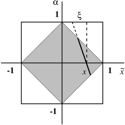
FIG. 1.: Graphical representation of the reduction formulas, Eq.(151), defining the SPD’s, $H(x,\xi)$ and $A(x,\xi)$, in terms of the double distribution, $f(\tilde{x},\alpha)$. The range of the arguments $\tilde{x}$ and $\alpha$ of the double distribution is the “rhombus” defined by $|\tilde{x}|+|\alpha|\leq 1$. The integration is over the line defined by the condition $\tilde{x}+\xi\alpha=x$ and lying inside the range of the variables $\tilde{x},\alpha$; it is indicated by the fat line. The variable $x$ defines the intersection of this line with the $\tilde{x}$–axis, the variable $\xi$ its deviation from the vertical. For $x=\xi$ the line runs through the upper corner of the rhombus.

As a consequence of the symmetries of the double distribution, Eqs.(133) and (134), the functions $H$ and $A$ satisfy the symmetry relations

$$\begin{array}[]{rcrrcr}H(x,\xi)&=&-H(-x,\xi),&\hskip 50.00008ptH(x,\xi)&=&H(x,-\xi),\\[8.61108pt] A(x,\xi)&=&A(-x,\xi),&A(x,\xi)&=&-A(x,-\xi).\end{array}$$ (152)

Furthermore, because of the antisymmetry of the combination $\alpha f(\tilde{x},\alpha)$ with respect both to $x$ and $\alpha$ we have

$$\int_{0}^{1}dx\,A(x,\xi)\;\;=\;\;0.$$ (153)

Note that the integral over $x$ is taken over the $0\leq x\leq 1$ interval. Hence, the distribution $A(x,\xi)$ cannot be a positive-definite function on $0\leq x\leq 1$.

Combining in Eq.(150) similar terms we obtain the following representation of the matrix element in terms of the skewed parton distributions:

$$\langle p-r/2|\left[\bar{\psi}(-z/2)\gamma_{\sigma}\psi(z/2)\right]^{\mbox{sym + total der.}}|p+r/2\rangle$$ (154)

$$= \int_{-1}^{1}dx\left(2p_{\sigma}e^{-ix(pz)}\left[H(x,\xi)-\frac{i(\Delta z)}{2}A(x,\xi)\right]\phantom{\int}\right.$$ (155)

$$+ \left.\left[\Delta_{\sigma}(pz)-p_{\sigma}(\Delta z)\right]\int_{0}^{1}dv\,v\,e^{-ivx(pz)}\left\{H(x,\xi)\,\sin[\bar{v}\xi(pz)]-iA(x,\xi)\,\cos[\bar{v}\xi(pz)]\right\}\right).$$ (156)

The cosine and sine functions can be represented as the sum or difference of exponentials. Combining them with the overall exponential factor, $e^{-ivx(pz)}$, one gets $vx\pm\bar{v}\xi$ combinations. However, using the symmetries in $x$ of the SPD’s, Eq.(152), one can easily arrange that only $vx+\bar{v}\xi$ appears. This finally gives

$$\langle p-r/2|\left[\bar{\psi}(-z/2)\gamma_{\sigma}\psi(z/2)\right]^{\mbox{sym + total der.}}|p+r/2\rangle$$ (157)

$$= \int_{-1}^{1}dx\left(2p_{\sigma}e^{-ix(pz)}\left[H(x,\xi)-\frac{i(\Delta z)}{2}A(x,\xi)\right]\phantom{\int}\right.$$ (158)

$$+ \left.\frac{i}{2}\,\left[\Delta_{\sigma}(pz)-p_{\sigma}(\Delta z)\right]\int_{0}^{1}dv\,v\,\left[e^{-i(vx+\bar{v}\xi)(pz)}+e^{i(vx+\bar{v}\xi)(pz)}\right]\left[H(x,\xi)-A(x,\xi)\right]\right).$$ (159)

The axial vector string operator. In a similar fashion we compute the matrix element of the axial vector string operator, Eq.(89). Substituting the double distribution part of the spectral representation of the contracted operator, Eq.(131), into Eq.(89), we obtain

$$\langle p-r/2|\left[\bar{\psi}(-z/2)\gamma_{\sigma}\gamma_{5}\psi(z/2)\right]^{\mbox{sym + total der.}}|p+r/2\rangle$$ (160)

$$= 2\epsilon_{\sigma\alpha\beta\gamma}z_{\alpha}r_{\beta}\int_{-1}^{1}d\tilde{x}\int_{-1+|\tilde{x}|}^{1-|\tilde{x}|}d\alpha\,f(\tilde{x},\alpha)\,\int_{0}^{1}dv\left[p_{\gamma}-ivk_{\gamma}(pz)\right]\,e^{-iv(kz)}\,\frac{\sin[\bar{v}(rz)/2]}{(rz)}.$$ (161)

Again integrating by parts in the $p_{\gamma}$ term, and keeping only terms linear in the transverse component of the momentum transfer, $\Delta$, this turns into

$$\langle p-r/2|\left[\bar{\psi}(-z/2)\gamma_{\sigma}\gamma_{5}\psi(z/2)\right]^{\mbox{sym + total der.}}|p+r/2\rangle$$ (162)

$$= \epsilon_{\sigma\alpha\beta\gamma}\,z_{\alpha}\Delta_{\beta}p_{\gamma}\int_{-1}^{1}d\tilde{x}\int_{-1+|\tilde{x}|}^{1-|\tilde{x}|}d\alpha\,f(\tilde{x},\alpha)\int_{0}^{1}dv\,v\,e^{-iv(\tilde{x}+\xi\alpha)(pz)}\left\{\cos[\bar{v}\xi(pz)]+{i\alpha}\,\sin[\bar{v}\xi(pz)]\right\}.$$ (163)

One sees that this matrix element can be expressed in terms of the same skewed distributions, $H$ and $A$, as the one of the vector operator:

$$\langle p-r/2|\left[\bar{\psi}(-z/2)\gamma_{\sigma}\gamma_{5}\psi(z/2)\right]^{\mbox{sym + total der.}}|p+r/2\rangle$$ (164)

$$= \frac{1}{2}\epsilon_{\sigma\alpha\beta\gamma}\,z_{\alpha}\Delta_{\beta}p_{\gamma}\int_{-1}^{1}dx\int_{0}^{1}dv\,v\,\left[e^{-i(vx+\bar{v}\xi)(pz)}-e^{i(vx+\bar{v}\xi)(pz)}\right]\left[H(x,\xi)-A(x,\xi)\right].$$ (165)

Hence, the matrix elements of both the vector and axial vector string operators, including the twist–2 and kinematical twist–3 contributions, are completely described by the two skewed distributions, $H$ and $A$, which, in turn, are determined by the original double distribution, Eq.(131), through the reduction formulas, Eq.(151).

Contribution from the PW–term. In order to obtain the full matrix elements of the vector and axial vector operator we must add to Eqs.(159) and (165) the parts coming from the PW–term in the spectral representation of the matrix element of the contracted operator, Eq.(131). Substituting this term in Eq.(89), and going through the same steps as described above for the double–distribution part, one easily sees that the contribution of the PW term to the matrix element of the vector operator is of the form

$$\langle p-r/2|\left[\bar{\psi}(-z/2)\gamma_{\sigma}\psi(z/2)\right]^{\mbox{sym + total der.}}|p+r/2\rangle_{\mbox{PW--Term}}\;\;=\;\;r_{\sigma}\int_{-1}^{1}d\alpha\,e^{-i\alpha(rz)/2}\,D(\alpha).$$ (166)

Note that the PW-term has a simple structure, corresponding to a parton picture in which the partons carry fractions $(1\pm\alpha)/2$ of the momentum transfer, $r$. Since only one momentum, $r$, is involved, this term can contribute only to the totally symmetric part of the vector string operator, and thus “decouples” in the reduction relations, Eqs.(60) and (60). For the same reason the PW term also does not contribute to the matrix element of the axial vector string operator: The derivatives with respect to both coordinates, $X$ and $z$, give rise to the momentum transfer, $r$, whence the contraction with the $\epsilon$–tensor gives zero.

C DVCS amplitude for pion target

Having at hands the parametrizations of the matrix elements of the vector and axial vector string operators we can now compute the DVCS amplitude for a pion target. Substituting the parametrizations, Eqs.(159) and (165), into Eq.(98), and performing the Fourier integral over the distance, $z$, we obtain the hadronic Compton amplitude in the form

$$T_{\mu\nu} = \int_{0}^{1}dx\int d^{4}z$$ (167)

$$;e^{i(qz)}\frac{2iz_{\rho}}{\pi^{2}(z^{2}-i0)^{2}}$$ (168)

$$\times \left\{2s_{\mu\rho\nu\sigma}p_{\sigma}\;e^{-ix(pz)}\;\left[H(x,\xi)-\frac{i(\Delta z)}{2}A(x,\xi)\right]\right.$$ (173)

$$+\;\frac{i}{2}\,s_{\mu\rho\nu\sigma}\left[\Delta_{\sigma}(pz)-p_{\sigma}(\Delta z)\right]$$

$$\;\;\;\;\;\times\int_{0}^{1}dv\,v\,\left[e^{-i(vx+\bar{v}\xi)(pz)}+e^{i(vx+\bar{v}\xi)(pz)}\right]\left[H(x,\xi)-A(x,\xi)\right]$$

$$-\;\frac{i}{2}\,\epsilon_{\mu\rho\nu\sigma}\epsilon_{\sigma\alpha\beta\gamma}\,z_{\alpha}\Delta_{\beta}p_{\gamma}$$

$$\left.\;\;\;\;\;\times\int_{0}^{1}dv\,v\,\left[e^{-i(vx+\bar{v}\xi)(pz)}-e^{i(vx+\bar{v}\xi)(pz)}\right]\left[H(x,\xi)-A(x,\xi)\right]\right\}$$

$$+ (q\rightarrow-q,\mu\leftrightarrow\nu).$$ (174)

Using the well–known identity for the contraction of two $\epsilon$–tensors one sees that the second and third term here can be combined to give two terms involving only exponential factors with positive and negative sign, respectively, which give identical contributions. The integral over $z$ is readily computed, using the basic formulas:

$$\int d^{4}z\,e^{i(lz)}\frac{z_{\rho}}{2\pi^{2}(z^{2}-i0)^{2}} = \frac{l_{\rho}}{l^{2}+i0},$$ (175)

$$\int d^{4}z\,e^{i(lz)}\frac{iz_{\rho}z_{\alpha}}{2\pi^{2}(z^{2}-i0)^{2}} = \frac{g_{\rho\alpha}l^{2}-2l_{\rho}l_{\alpha}}{(l^{2}+i0)^{2}}.$$ (176)

Here $l$ is to be replaced by the sum of all momenta appearing in the exponential factors, and $l^{2}$ in the denominators can be simplified using the special relations between invariants in DVCS kinematics, cf. Section II. Making use of the symmetry properties of the pion SPD’s, $H$ and $A$, Eq.(152), the result can be assembled in the form

$$T_{\mu\nu} = \frac{1}{2(pq)}\left\{\;2\left[p_{\mu}q_{\nu}+q_{\mu}p_{\nu}-g_{\mu\nu}(pq)+2\xi p_{\mu}p_{\nu}\right]\int_{-1}^{1}dx\frac{H(x,\xi)}{x-\xi+i0}\right.$$ (180)

$$\phantom{\frac{1}{2(pq)}}+\;\left[\Delta_{\mu}p_{\nu}+\Delta_{\nu}p_{\mu}\right]\int_{-1}^{1}dx\frac{A(x,\xi)}{x-\xi+i0}$$

$$\phantom{\frac{1}{(pq)}}+\;\int_{-1}^{1}dx[H(x,\xi)-A(x,\xi)]$$

$$\phantom{\frac{1}{2(pq)}}\;\;\;\;\;\left.\times\int_{0}^{1}dv\,v\,\left[\frac{q_{\mu}-(vx+\bar{v}\xi)p_{\mu}}{(\xi+vx+\bar{v}\xi-i0)^{2}}\Delta_{\nu}\;+\;\Delta_{\mu}\frac{q_{\nu}+(vx+\bar{v}\xi)p_{\nu}}{(-\xi+vx+\bar{v}\xi-i0)^{2}}\right]\right\}.$$

We can bring this result into a form which is manifestly transverse with respect to both the incoming and outgoing photon momenta. By simple algebraic rearrangement, and making use of the integral identity

$$\int_{0}^{1}dv\,v\,\frac{-vx-\bar{v}\xi}{(\xi+vx+\bar{v}\xi-i0)^{2}}+\frac{1}{x+\xi-i0} = \int_{0}^{1}dv\,v\,\frac{3\xi}{(\xi+vx+\bar{v}\xi-i0)^{2}},$$ (181)

which holds if $x\neq\pm\xi$, we first write Eq.(180) as a sum of three terms which are individually transverse [16]. In addition, we then perform an integration by parts in $x$ in order to remove the quadratic denominators. Here we use that

$$H(x,\xi)-A(x,\xi)\;\;=\;\;0\;\;\;\;\;\mbox{for}\;\;\;\;\;x\;\;=\;\;\pm 1,$$ (182)

which naturally follows from the reduction formulas, Eq.(151). In this way we finally obtain

$$T_{\mu\nu} = \frac{1}{2(pq)}\left\{\;2\left[p_{\mu}q_{\nu}+q_{\mu}p_{\nu}-g_{\mu\nu}(pq)+2\xi p_{\mu}p_{\nu}-p_{\mu}\frac{\Delta_{\nu}}{2}+\frac{\Delta_{\mu}}{2}p_{\nu}\right]\int_{-1}^{1}dx\frac{H(x,\xi)}{x-\xi+i0}\right.$$ (185)

$$\phantom{\frac{1}{2(pq)}}+\;(q_{\mu}+3\xi p_{\mu})\Delta_{\nu}\int_{-1}^{1}dx\int_{0}^{1}dv\,\frac{R(x,\xi)}{\xi+vx+\bar{v}\xi-i0}$$

$$\phantom{\frac{1}{2(pq)}}\left.+\;\Delta_{\mu}(q_{\nu}+\xi p_{\nu})\int_{-1}^{1}dx\int_{0}^{1}dv\,\frac{R(x,\xi)}{-\xi+vx+\bar{v}\xi+i0}\;\right\},$$

where $R(x,\xi)$ is a short–hand notation for the following combination of derivatives of the SPD’s:

$$R(x,\xi)\;\;\equiv\;\;\frac{\partial}{\partial x}H(x,\xi)-\frac{\partial}{\partial x}A(x,\xi).$$ (186)

All three terms here are individually transverse up to terms of order $t$. The decomposition of the Compton amplitude here is identical to the one introduced in Ref.[16]. The first term is the twist–2 part with the tensor structure corrected as suggested by Guichon and Vanderhaeghen [15]. The second and third term represent twist–3 contributions. Note that the second term contributes only to the helicity amplitude for a longitudinally polarized initial (virtual) photon, the third term for a transversely polarized one.

One observes that the second SPD, $A(x,\xi)$, enters in Eq.(185) only through its first derivative, cf. Eq.(186). From the reduction formulas, Eq.(151), one sees that the $x$–derivative of the function $A$ is related to the $\xi$–derivative of $H$ by

$$\frac{\partial}{\partial x}A(x,\xi)\;\;=\;\;-\frac{\partial}{\partial\xi}H(x,\xi),$$ (187)

so that instead of Eq.(186) one could equivalently write

$$R(x,\xi)\;\;=\;\;\left(\frac{\partial}{\partial x}+\frac{\partial}{\partial\xi}\right)H(x,\xi).$$ (188)

One could thus express the amplitude, Eq.(185), completely in terms of the first SPD, $H$, and its $\xi$–derivative. In this way one would obtain the form of the Compton amplitude given in Ref.[20].

Inspecting the singular integrals. We now inspect the singular integrals which appear in the the expression for the Compton amplitude, Eq.(185). The integrand in the first term has only a simple pole at $x=\xi$; this integral is of the same type as that obtained keeping only the twist–2 part of the matrix elements. The integral exists if the SPD, $H$, is continuous at $x=\xi$, which is the case for SPD’s derived from DD’s which are less singular than $1/\tilde{x}^{2}$ for $\tilde{x}\rightarrow 0$ and otherwise continuous [32]. The second and third term in Eq.(185) involve additional parameter integrals, so their convergence needs to be investigated carefully. In the second term, which contributes to the helicity amplitude for longitudinal polarization, we can perform the parameter integral over $v$, excluding the value $x=\xi$ for the moment:

$$\int_{0}^{1}\frac{dv}{\xi+vx+\bar{v}\xi-i0}\;\;=\;\;\frac{1}{x-\xi}\ln\left(\frac{x+\xi-i0}{2\xi-i0}\right).$$ (189)

This function has a logarithmic singularity at $x=-\xi$, while it is regular at $x=\xi$. The integral over $x$ in Eq.(185) exists if $R(x,\xi)$ is bounded at $x=-\xi$, which again is the case in the DD–based models described in Ref.[32]. We thus obtain a finite answer also for the second term contributing to longitudinal photon polarization.

Let us now turn to the third term of Eq.(185). Here we are dealing with an integral of the type (remember that $\bar{v}=1-v$)

$$\int_{0}^{1}\frac{dv}{-\xi+vx+\bar{v}\xi+i0}\;\;=\;\;\int_{0}^{1}\frac{dv}{v(x-\xi)+i0}.$$ (190)

This integral exhibits a logarithmic divergence at the lower limit. One may hope to get a finite result only if the integral

$$I(\xi)\;\;\equiv\;\;\int_{-1}^{1}dx\frac{R(x,\xi)}{x-\xi+i0}$$ (191)

vanished. However, one can easily convince oneself that this quantity is generally non-zero. In fact, representing $R(x,\xi)$ as in Eq.(188), and performing an integration by parts in the term with the $x$–derivative, one finds that

$$I(\xi)\;\;=\;\;\frac{d}{d\xi}\int_{-1}^{1}dx\frac{H(x,\xi)}{x-\xi+i0},$$ (192)

which is the $\xi$–derivative of the twist–2 contribution to the DVCS amplitude. Since the latter generally has a nontrivial $\xi$–dependence, determined by the shape of the SPDs, we conclude that the parameter integral Eq.(190) really is divergent. Thus, in our approximation the twist–3 part of the tensor amplitude $T_{\mu\nu}$ corresponding to transverse polarization of the initial photon contains a divergence. A similar observation has recently been made by Kivel et al. [20].

Absence of divergences in the physical DVCS amplitude. One may wonder if the divergence occurring in the tensor amplitude for transverse polarization of the initial photon affects the physical DVCS amplitude. Fortunately, this is not so. One can easily see that the tensor structure of the third term of Eq.(185) involving the divergent integral,

$$\Delta_{\mu}(q_{\nu}+\xi p_{\nu}),$$ (193)

is just a truncated (to first order in $\Delta$) version of the exactly gauge invariant combination,

$$\Delta_{\mu}{q_{2}}_{\nu}\;\;=\;\;\Delta_{\mu}(q_{\nu}+r_{\nu}/2)\;\;=\;\;\Delta_{\mu}(q_{\nu}+\xi p_{\nu}+\Delta_{\nu}/2),$$ (194)

which has zero projection on the polarization vector of the final real photon, $\epsilon_{2\nu}$: $(\epsilon_{2}q_{2})=0$. In fact, the structure $\Delta_{\mu}{q_{2}}_{\nu}$ is what one would obtain if one calculated the DVCS amplitude directly from the original “unexpanded” form of the DD parametrization of the matrix element, Eq.(147). It appears from the term with the exponential factor of the argument

$$-i[v(\tilde{x}+\xi\alpha)(pz)+\bar{v}\xi(pz)+(v\alpha+\bar{v})(\Delta z)/2],$$ (195)

which is obtained by combining the sine/cosine functions and the exponential factor in the second term of Eq.(147). In the Compton amplitude, this term gives rise to a contribution in which the argument of the quark propagator is

$$q+v(\tilde{x}+\xi\alpha)p+\bar{v}\xi p+(v\alpha+\bar{v})\Delta/2.$$ (196)

Since $(\Delta q),(\Delta p$) and $\Delta^{2}$ are negligible, the denominator factors in Eq.(185) remain the same as above. In the numerators, however, writing $(v\alpha+\bar{v})\Delta/2$ as $[1-(1-\alpha)v]\Delta/2$, we observe that the $\Delta_{\mu}(q_{\nu}+\xi p_{\nu})$ term of the above result converts into $\Delta_{\mu}(q_{\nu}+\xi p_{\nu}+\Delta_{\nu}/2)=\Delta_{\mu}{q_{2}}_{\nu}$, plus a contribution of the form $v\Delta_{\mu}\Delta_{\nu}$. The latter corresponds to a “new” SPD defined by a reduction formula of the type of Eq.(151) but with integrand $(1-\alpha)^{2}f(\tilde{x},\alpha)$. Due to the extra factor $v$, the $v$–integral for the latter contribution is finite. Thus, inclusion of the $\Delta_{\mu}\Delta_{\nu}$ term in the matrix elements and the Compton amplitude relegates the divergence in the tensor amplitude to the (exactly) unphysical part which does not contribute to the photon helicity amplitudes.

It may appear that retaining the $\Delta_{\mu}\Delta_{\nu}$ term in the Compton amplitude would exceed the accuracy of our approximation, since this term is formally of order $t$, and thus of the same order as corrections from $z^{2}$–terms in the matrix elements which we did not take into account. However, the $\Delta_{\mu}\Delta_{\nu}$ term is distinct in the sense that it can only arise in the way described above, i.e., from keeping finite $\Delta$ in the exponents of the matrix elements, while $z^{2}$–terms in the matrix elements can give rise only to corrections of order $t/q^{2}$ to already existing tensor structures. In this sense the inclusion of $z^{2}$–terms would not spoil the above argument proving that the physical Compton amplitude is divergence–free up to terms of order $t/q^{2}$.

To summarize, for the physical DVCS amplitude (i.e., the photon helicity amplitudes) we find no evidence for factorization breaking in the kinematical twist–3 contributions, both in the $\sqrt{t/q^{2}}$ and $t/{q^{2}}$ terms. It is quite possible that factorization breaks down at the $t/{q^{2}}$ level, but in order to establish this one would need to analyze the contributions from $z^{2}$–suppressed terms in the matrix element (i.e., twist–4 contributions).

Contribution from the PW–term. The complete result for the Compton amplitude includes also the contribution from the PW term. Since this part of the matrix element of the contracted operator “decouples” and does not produce kinematical twist–3 terms, its contribution to the Compton amplitude should be transverse by itself. Indeed, a straightforward calculation, making use of the symmetry Eq.(135), gives

$$T_{\mu\nu}|_{\mbox{PW--Term}}\;\;=\;\;\frac{1}{(rq)}\left[r_{\mu}q_{\nu}+q_{\mu}r_{\nu}-g_{\mu\nu}(rq)+r_{\mu}r_{\nu}\right]\;\int_{-1}^{1}d\alpha\;\frac{D(\alpha)}{1-\alpha},$$ (197)

which evidently satisfies

$$q_{\mu}T_{\mu\nu}|_{\mbox{PW--Term}}\;\;=\;\;0,\hskip 50.00008ptr_{\mu}T_{\mu\nu}|_{\mbox{PW--Term}}\;\;=\;\;O(t/q^{2}).$$ (198)

Hence this term can be regarded as a separate contribution. Alternatively, one may include the contribution from the PW–term into the basic SPD $H(x,\xi)$ and all SPD’s derived from it. Specifically, for $\xi>0$, the PW contribution to $H(x,\xi)$ is $D(x/\xi)\,\theta(|x|\leq\xi)$ [9]; it contributes $(\xi-x)D^{\prime}(x/\xi)\,\theta(|x|\leq\xi)/\xi^{2}$ [where $D^{\prime}(\alpha)\equiv(d/d\alpha)D(\alpha)]$ to $R(x,\xi)$. Inserting these functions into Eqs. (185) and (218) one rederives Eq. (197). One can also observe that the PW term makes zero contribution to $I(\xi)$, Eq. (191).

D Wandzura–Wilczek–type representation of twist–3 SPD’s

We can express the results for the matrix elements and the Compton amplitude derived in Sections IV B and IV C in an alternative form, introducing new skewed distributions as Wandzura–Wilczek–type transformations of the original SPD’s, $H$ and $A$. This allows us to demonstrate that our approach is equivalent to the Wandzura–Wilczek approximation proposed in Ref.[18]. In this language, the singularity for transverse photon polarization described in Section IV C appears due to discontinuities of the new SPD’s at $x=\xi$.

Within our approach the step leading to a Wandzura–Wilczek–type formulation is to introduce in the parameter integrals over $v$ the combination

$$vx+\bar{v}\xi$$ (199)

as a new variable. With $R(x,\xi)$ given by Eq.(186), we define a “transformed” function by way of

$$R_{W}(x,\xi) \equiv \int_{-1}^{1}dy\,R(y,\xi)\int_{0}^{1}dv\,\delta(yv+\bar{v}\xi-x)$$ (200)

$$= \theta(x\geq\xi)\int_{x}^{1}dy\;\frac{R(y,\xi)}{y-\xi}\;-\;\theta(x\leq\xi)\int_{-1}^{x}dy\;\frac{R(y,\xi)}{y-\xi}.$$ (201)

where $x\neq\xi$. Note that the function

$$R(x,\xi)\;\;=\;\;\frac{\partial}{\partial x}\left[H(x,\xi)-A(x,\xi)\right]$$ (202)

is continuous at $x=\xi$. This important property comes about as follows: As can be seen from the graphical representation of the reduction formula, Fig. 1, $x=\xi$ corresponds to the point where integration contour in Eq.(151) passes through the upper corner of the “rhombus” representing the two–dimensional region of support of the double distribution, $f(\tilde{x},\alpha)$. For a general double distribution, which not necessarily vanishes at $\alpha=\pm|\tilde{x}|$, the SPD’s $H$ and $A$ individually will be continuous at $x=\xi$, while their first derivative in $x$ will generally have a finite discontinuity. However, the difference, $H-A$, can be written as an integral of the type of Eq.(151) but with a factor of $1-\alpha$, which suppresses the contributions located in the corner of the integration region. As a result, not only the function $H-A$ but also its first derivative in $x$ are continuous at $x=\xi$.

Matrix elements of vector–type string operators in terms of the transformed SPD $R_{W}$. In terms of the new function, $R_{W}$, we can express the matrix elements of the vector and axial vector operators, Eqs.(159) and (165), as

$$\langle p-r/2|\left[\bar{\psi}(-z/2)\gamma_{\sigma}\psi(z/2)\right]^{\mbox{sym + total der.}}|p+r/2\rangle$$ (203)

$$= \int_{-1}^{1}dx\,e^{-ix(pz)}\left\{2p_{\sigma}\left[H(x,\xi)-\frac{i(\Delta z)}{2}A(x,\xi)\right]\right.$$ (204)

$$+ \left.\frac{1}{2}\,\left[\Delta_{\sigma}-p_{\sigma}\frac{(\Delta z)}{(pz)}\right]\left[R_{W}(x,\xi)-R_{W}(-x,\xi)\right]\right\},$$ (205)

$$\langle p-r/2|\left[\bar{\psi}(-z/2)\gamma_{\sigma}\gamma_{5}\psi(z/2)\right]^{\mbox{sym + total der.}}|p+r/2\rangle$$ (206)

$$= \frac{i}{2}\,\epsilon_{\sigma\alpha\beta\gamma}\,\frac{z_{\alpha}}{(pz)}\Delta_{\beta}p_{\gamma}\int_{-1}^{1}dx\,e^{-ix(pz)}\left[R_{W}(x,\xi)+R_{W}(-x,\xi)\right].$$ (207)

Note that only the odd part of $R_{W}(x,\xi)$ contributes to the vector operator, Eq.(205), and only the even part to the axial vector one, Eq.(207). [We remind that the full vector matrix element includes also the contribution from the PW–term, Eq.(166), which remains unchanged.]

We can now establish the relation of our functions to the twist–3 SPD’s introduced within the collinear expansion approach by Anikin et al. [16]. In Ref.[16] the matrix elements of the vector and axial vector operator were parametrized in the form (using our notation)

$$\frac{1}{2}\int\frac{d\lambda}{2\pi}e^{i\lambda x}\langle p-r/2|\bar{\psi}(-\lambda n/2)\left\{\begin{array}[]{c}\gamma_{\sigma}\\[6.45831pt] \gamma_{\sigma}\gamma_{5}\end{array}\right\}\psi(\lambda n/2)|p+r/2\rangle = \left\{\begin{array}[]{r}p_{\sigma}H_{1}(x,\xi)-\Delta_{\sigma}H_{3}(x,\xi),\\[6.45831pt] {\displaystyle\frac{i}{4}}\,\epsilon_{\sigma\alpha\beta\gamma}\,n_{\alpha}\Delta_{\beta}p_{\gamma}\,H_{A}(x,\xi).\end{array}\right.$$ (212)

where $n$ is a light–like vector, $n^{2}=0$, normalized as $(pn)=1$, and $(\Delta n)=0$. Setting in Eqs.(205) and (207) $z=\lambda n$, so that the terms proportional $(\Delta z)$ drop out, and comparing with Eqs.(212) we find that the Wandzura–Wilczek–type parts of these functions are given by

$$H_{1}(x,\xi)^{\rm W.W.} = H(x,\xi),$$ (213)

$$H_{3}(x,\xi)^{\rm W.W.} = -\frac{1}{4}\left[R_{W}(x,\xi)-R_{W}(-x,\xi)\right],$$ (214)

$$H_{A}(x,\xi)^{\rm W.W.} = \phantom{-}\frac{1}{4}\left[R_{W}(x,\xi)+R_{W}(-x,\xi)\right].$$ (215)

Compton amplitude in terms of the transformed SPD $R_{W}$. We can also express the Compton amplitude in terms of the new function, Eq.(201). This can be done either by computing the Compton amplitude as in Section IV C, using the parametrizations Eqs.(205) and (207) for the matrix elements of the vector–type operators, or directly by rewriting the old result, Eq.(185), in terms of the new SPD, Eq.(201). We obtain

$$T_{\mu\nu} = \frac{1}{2(pq)}\left\{\;2\left[p_{\mu}q_{\nu}+q_{\mu}p_{\nu}-g_{\mu\nu}(pq)+2\xi p_{\mu}p_{\nu}-\frac{\Delta_{\mu}}{2}p_{\nu}+p_{\mu}\frac{\Delta_{\nu}}{2}\right]\int_{-1}^{1}dx\frac{H(x,\xi)}{x-\xi+i0}\right.$$ (218)

$$\phantom{\frac{1}{2(pq)}}+\;(q_{\mu}+3\xi p_{\mu})\Delta_{\nu}\int_{-1}^{1}dx\,\frac{R_{W}(x,\xi)}{\xi+x-i0}$$

$$\phantom{\frac{1}{2(pq)}}\left.+\;\Delta_{\mu}(q_{\nu}+\xi p_{\nu})\int_{-1}^{1}dx\,\frac{R_{W}(x,\xi)}{-\xi+x+i0}\;\right\}.$$

To this one should add the contribution from the PW–term, Eq.(197), which remains unchanged.

Singular integrals with the transformed SPD $R_{W}$. Let us now inspect the singular integrals in the new representation of the Compton amplitude, Eq.(218). In particular, this will provide an alternative explanation of the divergence observed in Section IV C. In the second term, contributing to the amplitude for longitudinal photon polarization, the integral converges, since $R_{W}(x,\xi)$ is continuous at $x=-\xi$. This follows immediately from the integral definition of $R_{W}$, Eq.(201), and the fact that the function $R(x,\xi)$ in the integrand is bounded at $x=-\xi$. In the third term, however, contributing to the amplitude for transverse photon polarization, the integral with the singular function $1/(x-\xi+i0)$ would converge only if the function $R_{W}(x,\xi)$ were continuous at $x=\xi$. However, according to the definition, Eq.(201), $R_{W}$ is given by the integral of the function $R(y,\xi)/(y-\xi)$ from $x$ to 1 if $x>\xi$, and from $x$ to $-1$ if $x<\xi$. Hence there is no a priori reason why the limiting values of $R_{W}(x,\xi)$ when approaching $x=\xi$ from below and from above should coincide. In fact, the difference of the two limiting values can be written as a principal value integral:

$$R_{W}(\xi+0,\xi)-R_{W}(\xi-0,\xi)\;\;=\;\;{\rm P}\int_{-1}^{1}dy\;\frac{R(y,\xi)}{y-\xi},$$ (219)

which is generally non-zero [in fact, this is just the real part of the integral Eq.(191)]. We thus conclude that in this term the $x$–integral is divergent. Thus, our conclusions regarding the existence of the singular integrals in the terms contributing for longitudinal and transverse polarization are the same as those made in Section IV C. This should be so; after all, the introduction of the Wandzura–Wilczek–type SPD, $R_{W}$, merely corresponds to a change of integration variables in the integrals in the second and third terms of Eq.(185). Only the interpretation of the divergence is now different: It happens because of a discontinuity of the transformed function, $R_{W}(x,\xi)$, at $x=\xi$. As we have seen, this discontinuity is built into the transformation at a very elementary level; it is not contingent on any dynamical properties of the underlying SPD’s, $H$ and $A$. This is in accordance with the fact that in the formulation of Section IV C the divergence in the $v$–integral is not influenced by the behavior of the SPD’s.

V Conclusions

In this paper we have studied the DVCS amplitude at tree level, making use of the light–cone expansion in terms of QCD string operators in coordinate space. Let us summarize our main conclusions.

First, we have found that transversality of the light–cone expansion can be maintained by including in addition to the twist–2 operators a minimal set of “kinematical” twist–3 operators, which appear as total derivatives of twist–2 operators. The “dynamical” twist–3 contribution from quark–gluon operators is not involved in restoring transversality of the twist–2 contribution; the contribution from quark–gluon operators should be separately transverse once also their total derivatives are included (this can be done by generalizing the iterative procedure described in Section III B and Appendix A). From the point of view of transversality alone it is thus a legitimate approximation to neglect this contribution. In this sense the original appeal of DVCS as a process describable in terms of a small set of twist–2 non-forward matrix elements, closely related to the parton distribution of DIS, is preserved.

Second, we have found that retaining only the “kinematical” twist–3 contribution required by transversality leads to a finite result for the tensor amplitude corresponding to longitudinal polarization of the initial (virtual) photon. The tensor amplitude for transverse polarization contains a divergence already at tree level, whose origin are contributions with vanishing “longitudinal” component (in the parton model sense) of the momentum of the quark propagator. This divergence is specific to DVCS kinematics (technically speaking, they occur only if $\eta=\xi$) and are absent for finite virtuality of the outgoing photon. However, we found that the divergent part of the tensor amplitude has zero projection on the polarization vector of the outgoing (real) photon. Thus, in both cases (longitudinally or transversely polarized initial photon) the physical helicity amplitudes are finite. In this sense the approximation of keeping only the “kinematical” twist–3 contributions is consistent with the factorization of the DVCS amplitude. It may thus be used for estimating observables such as the DVCS cross section, the contribution from interference of DVCS with the Bethe–Heitler process, spin and charge asymmetries, etc.

Our results can serve as a basis for computing kinematical power corrections to the DVCS amplitude, both of type $t/q^{2}$ and $m^{2}/q^{2}$, which are analogous to the well–known target mass corrections in DIS [29, 30]. In the coordinate–space approach these corrections can be incorporated in a very elegant way, by including terms of order $z^{2}$ in the parametrizations of the matrix elements of the twist–2 operators. The latter are obtained by solving the harmonic condition on the matrix elements, Eq.(41) [13, 36].

In this paper we have computed the DVCS amplitude for the pion (more precisely, its isoscalar component), taking advantage of the fact that the pion has spin zero and definite $C$–parity. The generalization of the approach described in Section IV to the more realistic case of the nucleon is straightforward. The parametrization of the nucleon matrix elements of the twist–2 string operators in terms of double distributions and a PW–term has been discussed in Refs.[9, 22]. In particular, this will allow to study the influence of the “kinematical” twist–3 contributions on the sum rules relating the nucleon SPD’s in the forward limit to the quark orbital angular momentum in the nucleon [1].

VI Acknowledgements

We are grateful to I.I. Balitsky, J. Blümlein, V.M. Braun, M. Diehl, B. Geyer, N. Kivel, M. Lazar, D. Müller, I. Musatov, M.V. Polyakov, and O. Teryaev for many interesting discussions ad helpful hints. While this work was being completed the article of Belitsky and Müller appeared [18], where a similar recursive method for inclusion of the “kinematical” twist–3 contributions is described. The divergences in the amplitude for transverse photon polarization were also noted recently by Kivel et al. [20]. The generalization to the case of a nucleon target has been discussed in Ref.[37].

A Deconstructing the string operators

In this appendix we demonstrate how the operator relations Eqs.(57) and (60), expressing the vector string operator through its symmetric part and the total derivative of the string operator of opposite parity, can be solved recursively, giving rise to the closed–form expression stated in Eq.(84). As explained in Section III B, we shall not consider the quark–gluon operators appearing in the reduction process, since they are not needed to maintain transversality of the light–cone expansion. In principle, of course, generalizing the technique described below, the operator relations could be solved keeping also the quark–gluon operators.

For brevity let us introduce the following notation for the basic (unsymmetrized) vector and axial vector string operators:

$$\left.\begin{array}[]{c}S_{\sigma}(z|X)\\[6.45831pt] S_{5\sigma}(z|X)\end{array}\right\}\;\;\equiv\;\;\bar{\psi}(X-z/2)\left\{\begin{array}[]{c}\gamma_{\sigma}\\[6.45831pt] \gamma_{\sigma}\gamma_{5}\end{array}\right\}\psi(X+z/2).$$ (A1)

The R.H.S. of the relations Eqs.(57) and (60) can be regarded as the action of a certain linear integral operator on the string operators:

$$({\cal L}S)_{\sigma}(z|X)\;\;\equiv\;\;\frac{1}{2}\epsilon_{\sigma\alpha\beta\gamma}z_{\alpha}R_{\beta}\int_{0}^{1}dt\,t\;S_{\gamma}(tz|X),$$ (A2)

where

$$R_{\beta}\;\;\equiv\;\;i\frac{\partial}{\partial X_{\beta}}.$$ (A3)

With the help of this formal operator, Eqs.(57) and (60), with the quark–gluon operators neglected, can be written in compact form:

$$-({\cal L}S)_{\sigma}\;+\;S_{5\sigma} = S^{\rm sym}_{5\sigma},$$ (A4)

$$-({\cal L}S_{5})_{\sigma}\;+\;S_{\sigma} = S^{\rm sym}_{\sigma}.$$ (A5)

These equations decouple if one introduces instead of the vector and axial vector type string operators the left– and right–handed combinations $(S_{\sigma}\pm S_{5\sigma})/2$; the decoupling is, of course, a consequence of chiral invariance of QCD. The formal solution of the system Eqs.(A4) and (A5) is

$$S_{\sigma} = \left(\frac{1}{1-{\cal L}^{2}}S^{\rm sym}\right)_{\sigma}\;+\;\left(\frac{{\cal L}}{1-{\cal L}^{2}}S_{5}^{\rm sym}\right)_{\sigma},$$ (A6)

$$S_{5\sigma} = \left(\frac{1}{1-{\cal L}^{2}}S_{5}^{\rm sym}\right)_{\sigma}\;+\;\left(\frac{{\cal L}}{1-{\cal L}^{2}}S^{\rm sym}\right)_{\sigma}.$$ (A7)

These relations allow to express the full string operators in terms of totally symmetrized (i.e., twist–2) operators. The inverse of the linear operator $1-{\cal L}^{2}$ here is understood in the sense of a series expansion:

$$\frac{1}{1-{\cal L}^{2}} = 1+{\cal L}^{2}+{\cal L}^{4}+\ldots$$ (A8)

$$\frac{{\cal L}}{1-{\cal L}^{2}} = {\cal L}+{\cal L}^{3}+{\cal L}^{5}+\ldots$$ (A9)

By iterating the operator ${\cal L}$ one can easily convince oneself that the even and odd powers of ${\cal L}$ observe the following patterns ($n\geq 1$):

$$({\cal L}^{2n}S)_{\sigma} = \frac{(-1)^{n-1}}{2(2n-1)!}\left[R_{\sigma}z_{\gamma}-(Rz)g_{\sigma\gamma}\right]\left[\frac{(Rz)}{2}\right]^{2n-1}\int_{0}^{1}dv\;v\bar{v}^{2n-1}\;S_{\gamma}(vz),$$ (A10)

$$({\cal L}^{2n-1}S)_{\sigma} = \frac{(-1)^{n-1}}{2(2n-2)!}\epsilon_{\sigma\alpha\beta\gamma}z_{\alpha}R_{\beta}\left[\frac{(Rz)}{2}\right]^{2n-2}\int_{0}^{1}dv\;\;v\bar{v}^{2n-2}\;S_{\gamma}(vz).$$ (A11)

These expressions apply up to terms involving operators of the form

$$R^{2}S_{\gamma}\hskip 20.00003pt\mbox{or}\hskip 20.00003ptR_{\gamma}S_{\gamma},$$ (A12)

whose matrix elements in DVCS kinematics are proportional to $t$ or $m^{2}$. More rigorously, Eqs.(A10) and (A11) can be proven be induction. Obviously, Eq.(A11) with $n=1$ describes the first power of the operator, ${\cal L}$, Eq.(A2). Acting on Eq.(A11) (for general $n$) with ${\cal L}$ we have to remember that Eq.(A2) implies that the distance, $z$, is to be rescaled by the parameter, $t$, everywhere, not only in the arguments of the fields, so that we pick up a total factor of $t^{2n-1}$. We thus obtain:

$$[{\cal L}({\cal L}^{2n-1}S)]_{\sigma} = ({\cal L}^{2n}S)_{\sigma}\;\;=\;\;\frac{(-1)^{n-1}}{4(2n-2)!}\epsilon_{\sigma\alpha\beta\gamma}\epsilon_{\gamma\alpha^{\prime}\beta^{\prime}\gamma^{\prime}}z_{\alpha}z_{\alpha^{\prime}}R_{\beta}R_{\beta^{\prime}}$$ (A14)

$$\times\left[\frac{(Rz)}{2}\right]^{2n-2}\int_{0}^{1}dt\,t^{2n}\int_{0}^{1}du\,u\bar{u}^{2n-2}\;S_{\gamma^{\prime}}(tuz).$$

Using the well–known expression for the contraction of two $\epsilon$–tensors we find

$$\epsilon_{\sigma\alpha\beta\gamma}\epsilon_{\gamma\alpha^{\prime}\beta^{\prime}\gamma^{\prime}}z_{\alpha}z_{\alpha^{\prime}}R_{\beta}R_{\beta^{\prime}}\;\;=\;\;(Rz)\left[R_{\sigma}z_{\gamma^{\prime}}-(Rz)g_{\sigma\gamma^{\prime}}\right]\;+\;\mbox{terms $\propto R^{2},R_{\gamma^{\prime}}$}.$$ (A15)

The parameter integral in Eq.(A14) can be simplified by introducing a new variable, $v\equiv tu$:

$$\int_{0}^{1}dt\,t^{2n}\int_{0}^{1}du\,u(1-u)^{2n-2}\;S_{\gamma^{\prime}}(tuz)$$ (A16)

$$= \int_{0}^{1}dt\,\int_{0}^{t}dv\,v(t-v)^{2n-2}\;S_{\gamma^{\prime}}(vz)$$ (A17)

$$= \int_{0}^{1}dv\,\int_{v}^{1}dt\,v(t-v)^{2n-2}\;S_{\gamma^{\prime}}(vz)$$ (A18)

$$= \frac{1}{2n-1}\int_{0}^{1}dv\,v(1-v)^{2n-1}\;S_{\gamma^{\prime}}(vz).$$ (A19)

Combining these statements we see that Eq.(A14) is indeed equal to the proposed expression, Eq.(A10). In an analogous way one shows that acting on Eq.(A10) with ${\cal L}$ one reproduces Eq.(A11) with $n$ replaced by $n+1$.

From Eqs.(A10) and (A11) we see that the series of even and odd powers of the operator, ${\cal L}$, Eqs.(A8) and (A9), have the form of the power series of the sine and cosine functions, respectively:

$$\sum_{n=1}^{\infty}\frac{(-1)^{n-1}}{(2n-1)!}\left[\bar{v}\frac{(Rz)}{2}\right]^{2n-1} = \sin\left[\bar{v}\frac{(Rz)}{2}\right],$$ (A20)

$$\sum_{n=1}^{\infty}\frac{(-1)^{n-1}}{(2n-2)!}\left[\bar{v}\frac{(Rz)}{2}\right]^{2n-2} = \cos\left[\bar{v}\frac{(Rz)}{2}\right].$$ (A21)

Substituting this in Eqs.(A6), (A7) we finally obtain [cf. Eq.(84)]:

$$S_{\sigma}(z) = S_{\sigma}^{\rm sym}(z)\;+\;\frac{1}{2}\left[R_{\sigma}z_{\gamma}-(Rz)g_{\sigma\gamma}\right]\;\int_{0}^{1}dv\,v\;\sin\left[\bar{v}\frac{(Rz)}{2}\right]S_{\gamma}^{\rm sym}(vz)$$ (A22)

$$+ \frac{1}{2}\epsilon_{\sigma\alpha\beta\gamma}z_{\alpha}R_{\beta}\;\int_{0}^{1}dv\,v\;\cos\left[\bar{v}\frac{(Rz)}{2}\right]S_{5\gamma}^{\rm sym}(vz),$$ (A23)

and an analogous result with $S$ and $S_{5}$ interchanged. Note that this expression applies up to operators of the form Eq.(A12), which give power–suppressed contributions to the DVCS amplitude.

We remind again that the full expression for the string operator contains also quark–gluon string operators, which upon symmetrization produce operators of twist $\geq 3$. We have not kept track of them, since they turn out not be essential for restoring transversality of the twist–2 contribution. In principle they could be included in the above iterative procedure.

REFERENCES

- [1] X. Ji, Phys. Rev. D55 (1997) 7114 [hep-ph/9609381].
- [2] J. C. Collins, L. Frankfurt and M. Strikman, Phys. Rev. D56 (1997) 2982 [hep-ph/9611433].
- [3] A. V. Radyushkin, Phys. Rev. D56 (1997) 5524 [hep-ph/9704207].
-
[4]
P. R. Saull [ZEUS Collaboration],
hep-ex/0003030;
P. Bussey [ZEUS Collaboration], Talk presented at the International Workshop on Skewed Parton Distributions and Lepton–Nucleon Scattering, DESY, Hamburg, Sep. 11-12, 2000. - [5] E. Lobodzinska [H1 Collaboration], Talk presented at the International Workshop on Skewed Parton Distributions and Lepton–Nucleon Scattering, DESY, Hamburg, Sep. 11-12, 2000.
- [6] M. Amarian [HERMES Collaboration], Talk presented at the International Workshop on Skewed Parton Distributions and Lepton–Nucleon Scattering, DESY, Hamburg, Sep. 11-12, 2000.
-
[7]
J. P. Chen et al.,
PCCF-RI-0013 (Proposal to Jefferson Lab PAC 18);
Ch. Hyde–Wright, Talk presented at the International Workshop on Skewed Parton Distributions and Lepton–Nucleon Scattering, DESY, Hamburg, Sep. 11-12, 2000. - [8] M. V. Polyakov, Nucl. Phys. B555 (1999) 231 [hep-ph/9809483].
- [9] M. V. Polyakov and C. Weiss, Phys. Rev. D60 (1999) 114017 [hep-ph/9902451].
- [10] M. Diehl, T. Gousset, B. Pire and O. Teryaev, Phys. Rev. Lett. 81 (1998) 1782 [hep-ph/9805380].
- [11] R. K. Ellis, W. Furmanski and R. Petronzio, Nucl. Phys. B212 (1983) 29.
- [12] S. A. Anikin and O. I. Zavyalov, Annals Phys. 116 (1978) 135.
- [13] I. I. Balitsky and V. M. Braun, Nucl. Phys. B311 (1989) 541.
- [14] J. Blumlein and D. Robaschik, Nucl. Phys. B581 (2000) 449 [hep-ph/0002071].
- [15] P.A.M. Guichon and M. Vanderhaeghen, Progr. Part. Nucl. Phys. 21 (1998) 125.
- [16] I. V. Anikin, B. Pire and O. V. Teryaev, Phys. Rev. D62, 071501 (2000) [hep-ph/0003203].
- [17] M. Penttinen, M. V. Polyakov, A. G. Shuvaev and M. Strikman, hep-ph/0006321.
- [18] A. V. Belitsky and D. Muller, hep-ph/0007031.
- [19] A. V. Radyushkin and C. Weiss, hep-ph/0008214.
- [20] N. Kivel, M. V. Polyakov, A. Schafer and O. V. Teryaev, hep-ph/0007315.
- [21] A. V. Radyushkin, Phys. Rev. D59 (1999) 014030 [hep-ph/9805342].
- [22] A. V. Radyushkin, Phys. Lett. B449 (1999) 81 [hep-ph/9810466].
- [23] J. Bartels and M. Loewe, Z. Phys. C12 (1982) 263.
- [24] B. Geyer, D. Robaschik, M. Bordag and J. Horejsi, Z. Phys. C26 (1985) 591.
- [25] F. M. Dittes, D. Muller, D. Robaschik, B. Geyer and J. Horejsi, Phys. Lett. B209 (1988) 325.
- [26] L. Frankfurt, A. Freund, V. Guzey and M. Strikman, Phys. Lett. B418 (1998) 345 [hep-ph/9703449]. Erratum ibid. B429 (1998) 414.
- [27] A. V. Belitsky, B. Geyer, D. Muller and A. Schafer, Phys. Lett. B421 (1998) 312 [hep-ph/9710427].
- [28] For a discussion of the mathematical aspects of twist decomposition see also: B. Geyer, M. Lazar, Nucl. Phys. B581 (2000) 341 [hep-th/0003080]; hep-ph/0009309
- [29] O. Nachtmann, Nucl. Phys. B63 (1973) 237.
- [30] H. Georgi and H. D. Politzer, Phys. Rev. D14 (1976) 1829.
- [31] L. Mankiewicz, G. Piller and T. Weigl, Eur. Phys. J. C 5, 119 (1998).
- [32] I. V. Musatov and A. V. Radyushkin, Phys. Rev. D61 (2000) 074027 [hep-ph/9905376].
- [33] V. Y. Petrov, P. V. Pobylitsa, M. V. Polyakov, I. Bornig, K. Goeke and C. Weiss, Phys. Rev. D57 (1998) 4325 [hep-ph/9710270].
- [34] S. Mandelstam, Proc. Roy. Soc. Lond. A233 (1955) 248.
- [35] F. Gross and D. O. Riska, Phys. Rev. C36 (1987) 1928.
- [36] I. I. Balitsky and V. M. Braun, Phys. Lett. B222 (1989) 123.
- [37] N. Kivel and M. V. Polyakov, hep-ph/0010150.