PATHOLOGICAL SCIENCE

Abstract

I discuss examples of what Dr. Irving Langmuir, a Nobel prize winner in Chemistry, called “the science of things that aren’t so.” Some of his examples are reviewed and others from High Energy Physics are added. It is hoped that discussing these incidents will help us develop an understanding of some potential pitfalls.

1 Introduction

Often, much more often than we would like, experimental results are reported that have impressive “statistical significance,” but are subsequently proven to be wrong. These results have labeled by Irving Langmuir as the “Science of things that aren’t so.” Langmuir described some of these incidents in a 1953 talk that was transcribed and may still be available.[1] Here I will repeat some of Langmuir’s examples, and show some other examples from High Energy Physics.

The examples shown here are not cases of fraud; the proponents believed in the work they presented. But they were wrong.

2 Davis-Barnes Effect

Circa 1930 Professors B. Davis and A. Barnes of Columbia University did an experiment where they produced $\alpha$ particles from the decay of Polonium and $e^{-}$ from a filament in an apparatus sketched in Fig. 1. The electrons are accelerated by a varying potential. At 590 V they move with the same velocity as the $\alpha$’s. Then they may combine with the $\alpha$’s to form a bound $\alpha-e^{-}$ “atomic state.” They then continue down the tube and are counted visually by making scintillations in the screens at Y or Z that viewed with a microscope.

Without a magnetic field all the $\alpha$’s reach the screen at Y. With a magnetic field and no accelerating voltage for the electrons they all reach the screen at Z. However, if the electrons bind with the doubly positive charged $\alpha$’s they would deflect half as much and not reach Z.

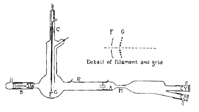
Figure 1: Diagram of first tube. S, radioactive source; W, thin glass window; F, filament; G, grid; R, lead to silvered surface; A, second anode; M, magnetic field; C, copper seals; Y and Z, zinc sulfide screens.

What they found was very extraordinary. Not only did the electrons combine with the $\alpha$’s at 590 V, but also at other energies “that were exactly the velocities that you calculate from Bohr theory.” Furthermore all the capture probabilities were about 80%. Their data are shown in Fig. 2.

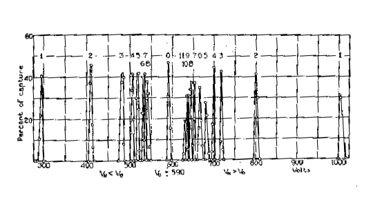
Figure 2: Electron capture as a function of accelerating voltage.

Now there is a problem here because in Bohr theory when an electron comes in from infinity it has to radiate half its energy to enter into orbit. There was no evidence for any such radiation and the electron would have needed to have twice the energy to start with. However, there were some theorists including Sommerfeld who had an explanation that the electron could be captured if it had a velocity equal to what it was going to have in orbit.

There were other disturbing facts. The peaks were 0.01 V wide; the fields in the tube were not that accurate. In addition, scanning the entire voltage range in such small steps would take a long time. Well, Davis and Barnes explained, they didn’t quite do it that way: they found by some preliminary work that they did check with the Bohr orbit velocities, so they knew where to look. Sometimes they weren’t quite in the right place, so they explored around and found them. Their precision was so good they were sure they could get a better value for the Rydberg constant (known then to 1 part in 10⁸).

Then Langmuir visited Columbia. The way the experiment was done was that an assistant named Hull sat opposite to Barnes in front of a voltmeter, that had a scale that went from 1 to a thousand volts and on that scale he was reading 0.01 V. The room was dark, to see the scintillations, and there was a light on the voltmeter and on the dial of the clock that Barnes used to time his measurements.

Langmuir says it best: “He said he always counted for two minutes. Actually, I had a stop watch and I checked him up. They sometimes were as low as one minute and ten seconds and sometimes one minute and fifty-five seconds, but he counted them all as two minutes, and yet the results were of high accuracy!

“And then I played a dirty trick. I wrote out on a card of paper ten different sequences of V and zero. I meant to put on a certain voltage and then take it off again. Later I realized that that wasn’t quite right because when Hull took off the voltage, he sat back in his chair—there was nothing to regulate at zero, so he didn’t. Well, of course, Barnes saw him whenever he sat back in his chair. Although, the light wasn’t very bright, he could see whether he was sitting back in his chair or not so he knew the voltage wasn’t on and the result was that he got a corresponding result. So later I whispered, ‘Don’t let him know that you’re not reading,’ and I asked him to change the voltage from 325 down to 320 V so he’d have something to regulate and I said, ‘regulate it just as carefully as if you were sitting on a peak.’ So he played the part from that time on, and from that time on Barnes’ readings had nothing whatever to do with the voltages that were applied. Whether the voltage was at one value or another didn’t make the slightest difference. I said ‘you’re through. You’re not measuring anything at all. You never have measured anything at all.’ ‘Well,’ he said, ‘the tube was gassy. The temperature has changed and therefore the nickel plates must have deformed themselves so that the electrodes are no longer lined up properly.’

“He immediately—without giving any thought to it—he immediately had an excuse. He had a reason for not paying any attention to any wrong results. It just was built into him. He just had worked that way all along and always would. There is no question but what he is honest; he believed these things, absolutely.”

In fact they did publish their results even after being confronted by Langmuir.[2] Later after no one else had been able to reproduce their results they published a retraction,[3] that said in part: “These results reported depended on observations made by counting scintillations visually. The scintillations produced by $\alpha$ particles on a zinc sulfide screen are a threshold phenomenon. It is possible that the number of counts may be influenced by external suggestion or autosuggestion to the observer. The possibility that the number of counts might be greatly influenced by suggestion had been realized, and a test of their reliability had been made by two methods: (a) The voltage applied to the electrons was altered without the knowledge of the observer (Barnes); (b) the direction of the electron stream with respect to the $\alpha$-particle path was altered by a small electro-magnet. Such changes in voltage and direction of electron stream were noted at once by the observer. These checks were thought at the time to be entirely adequate. In examining the data of observation made in our laboratory Dr. Irving Langmuir concluded that the checks applied had not been sufficient, and convinced us that the experiments should be repeated by wholly objective methods. Accordingly we have investigated the matter by means of the Geiger counter. Four additional experimental electron $\alpha$-ray tubes have been constructed for this purpose.

“Capture of the kind reported was often observed over a considerable period of time, but following prolonged observation the effect seemed to disappear. The results deduced from visual observations have not been confirmed. If such capture of electrons does take place, it must depend on unknown critical conditions which we were not able to reproduce at will in the new experimental tubes.”

It is interesting to note that they still seemed to be holding out the possibility that somehow the earlier results were correct.

3 N-rays

In 1903 there was a lot of experimentation with x-rays. Blondlot, a respected member of the French Academy of Sciences, found that if you have a hot wire heated inside an iron tube with a window cut out of it, rays would emerge that would get through aluminum. He call these N-rays.[4] They had specific properties. For example, they could get through 2” or 3” of aluminum but not through iron. The way he detected these rays was by observing an object illuminated with a faint light. When the N-rays were present you could “see the object much better.”

N-rays could be stored. Brick wrapped in black paper put in sunlight would store and reemit them, but the effect was independent of the number of bricks. Many other things would give off N-rays, including people. They even split when traversing an aluminum prism. Blondlot measured the index of refraction of the different components.

The American physicist R. W. Wood visited Blondlot’s laboratory and was shown the experiments. While Blondlot demonstrated his measurement of the refractive indicies, Wood palmed the prism. It did not affect the measurements. Wood cruelly published that,[5] and that was the end of Blondlot.

Now the question is how do we explain Blondlot’s findings. Pringsheim tried to repeat Blondlot’s experiments and focused on the detection method. He found that if you have a very faint source of light on a screen of paper and to make sure that you are seeing the screen of paper you hold your hand up and move it back and forth. And if you can see your hand move then you know it is illuminated. One of Blondlot’s observations was that you can see much better if you had some N-rays falling on the piece of paper. Pringsheim repeated these and found that if you didn’t know where the paper was, whether it was in front or behind your hand, it worked just as well. That is you could see your hand just as well if you held it back of the paper as if you held it in front. Which is the natural thing, because this is a threshold phenomenon, and a threshold phenomenon means that you don’t know, you really don’t know, whether you are seeing it or not. But if you have your hand there, well of course, you see your hand because you know your hand’s there, and that’s just enough to win you over to where you know that you see it. But you know it just as well if the paper happens to be in front of your hand instead of in back of your hand, because you don’t know where the paper is but you do know where your hand is.

4 Symptoms of Pathological Science

Langmuir lists six characteristics of pathological science:

1. The maximum effect that is observed is produced by a causative agent of barely detectable intensity, and the magnitude of the effect is substantially independent of the cause.

2. The effect is of a magnitude that remains close to the limit of detectability, or many measurements are necessary because of the low statistical significance of the results.

3. Claims of great accuracy.

4. Fantastic theories contrary to experience.

5. Criticisms are met by ad hoc excuses thought up on the spur of the moment.

6. Ratio of supporters to critics rises up to somewhere near 50% and then falls gradually to oblivion.

Let us go on to examples from high energy physics and see how these criteria apply. Unfortunately, there are many examples. I have just chosen a few.

5 The Split $A_{2}$ Meson Resonance

Two CERN experiments, the Missing Mass Spectrometer (MMS) experiment,[6] and the CERN Boson Spectrometer (CBS) experiment,[7] claimed that the structure around 1300 MeV, believed to be the $2^{+}$ $A_{2}$ meson produced in pion proton collisions did not have a simple Breit-Wigner form, as expected for a short lived resonance, but was in fact divided (or split) into two peaks. Their data are shown in Fig. 3.

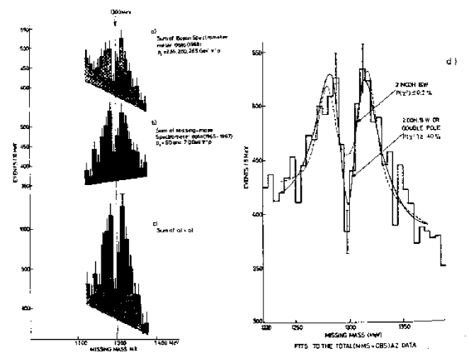
Figure 3: (a-c) Evidence for $A_{2}$ splitting in $\pi^{-}p\to pX^{-}$ collisions in the two CERN experiments, (d) same as (c) in 5 MeV bins fit to two hypotheses.

This indeed was a startling result with no obvious explanation. Such a resonance shape could mean new physics. The MMS experiment just observed the outgoing proton and thus computed the missing mass from proton and the knowledge of the incident $\pi^{-}$ beam. The CBS experiment could also observe the decay products of the $A_{2}$. Bubble chamber experiments also saw evidence for the splitting. Böckman et al. had 5 GeV/c $\pi^{+}p$ data.[8] They looked at the $\rho^{\circ}\pi^{+}$ final state and showed their data for a specific cut on the momentum transfer between the initial and final state proton ($t-t_{min}<0.1$). Their data shows a split (see Fig. 4). Anguilar-Benitez et al. [9] showed their $K^{\circ}K^{\pm}$ data which they claim fits best to a double pole (see Fig. 5). There were also inconclusive but split-suggestive data from Crennell et al.[10]

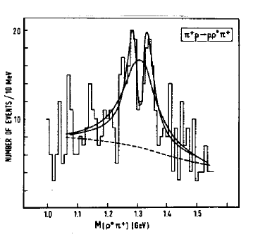
Figure 4: Data from Böckman et al.  The simple Breit-Wigner has a 20% probability while the double-pole fit gives 63%.

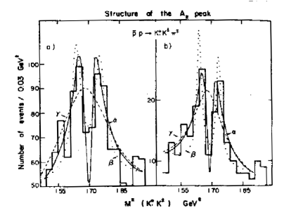
Figure 5: Data of Aguilar-Benitez et al. (a) All $\overline{p}$ momenta included (note the suppressed zero). (b) Only the 0.7 GeV/c data. Using (a) only, the fit for double-pole ($\alpha$) gives 65% likelihood.

A. Barbaro-Galtieri reviewed the situation at the 1970 Meson Spectroscopy conference.[11] At the time there was only one publicly available result that directly contradicted the split. These data, from a $\pi^{+}p$ bubble chamber experiment done by the Berkeley group (LRL), are compared with the MMS data in Fig. 6.[12]

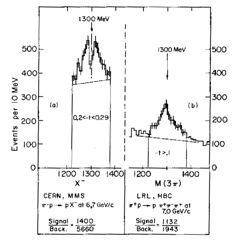
Figure 6: Comparison of MMS and LRL data at similar incident pion momenta. (a) MMS, resolution $\Gamma$/2=8.0 MeV, (b) LRL, resolution $\Gamma$/2=6.4 MeV.

At this conference doubt was raised about the validity of the split. Others then came forward.[13] There were new experiments.[14] By the 1972 Meson Spectroscopy conference, there was no mention of the split. It had vanished into oblivion.[15]

How did this happen? I have heard several possible explanations. In the MMS experiment, I was told that they adjusted the beam energy so the dip always lined up! Another possibility was revealed in a conversation I had with Schübelin, one of the CBS physicists. He said: “The dip was a clear feature. Whenever we didn’t see the dip during a run we checked the apparatus and always found something wrong.” I then asked him if they checked the apparatus when they did see the dip, and he didn’t answer.

What about the other experiments that did see the dip? Well there were several experiments that didn’t see it. Most people who didn’t see it had less statistics or poorer resolution than the CERN experiments, so they just kept quiet. Those that had a small fluctuation toward a dip worked on it until it was publishable; they looked at different decay modes or $t$ intervals, etc. (This is my guess.)

6 The R, S, T and U Bosons

The 1970 Meson Spectroscopy conference contained many new results involving claims for states of relatively narrow width in the 3 GeV mass region. The CBS group also presented evidence of significant peaks, more than four standard deviations for six new resonances above 2.5 GeV/c. Their data are shown in Fig. 7.[16]

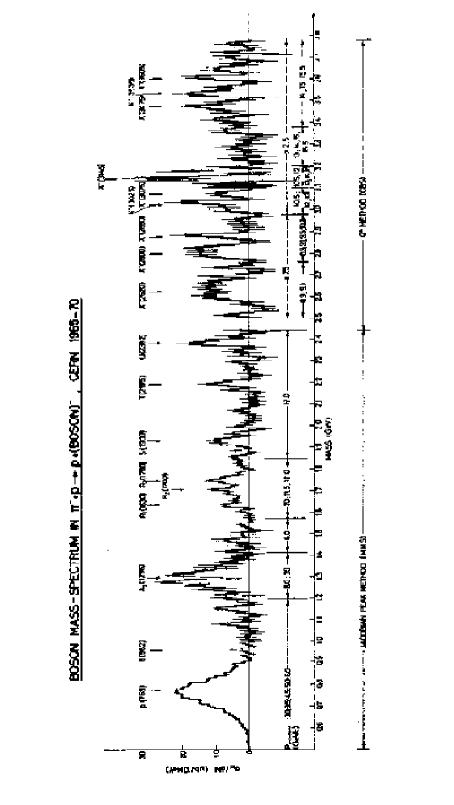
Figure 7: Compiled spectrum obtained by adding the spectra in different mass regions with the hand-drawn background subtracted. The arrows indicate the position of known or suspected particles.

Other groups also saw bumps. At the 1970 conference Miller reported similar structures seen in a 13 GeV/c incident momenta $\pi^{+}p$ bubble chamber experiment.[17] Kalbfleisch gave a review entitled “The T Region,” in which he stated “In this reiview paper I will discuss evidence for mesons in the T region (mass 2.19 GeV). The T^- is well known from the original missing mass spectrometer work at CERN.”[18]

Subsequently, there were no further confirmations of these signals. In fact, all of these bumps eventually went away.

7 The $F$ or $D_{s}$ Meson

The spin-0 meson formed from $c\overline{s}$ constituent quarks was called at first the $F$, but was renamed by the Particle Data Group as the $D_{s}$. The name was not changed to protect the innocent.[19] The $F$ decays mostly by having the $c$ quark transform to an $s$ quark and a virtual $W^{+}$ boson. In the simplest case, the $W^{+}$ manifests itself as a $\pi^{+}$ and the $s$ quark combines with the original $\overline{s}$ quark to form a $\phi$ or $\eta$ meson.

In 1977 the DASP group working at the DORIS $e^{+}e^{-}$ storage ring at DESY found a handful of events at a center-of-mass energy of 4.42 GeV that they classified as coming from the reaction $e^{+}e^{-}\to F^{+}F^{-}\gamma$, where the $\gamma$ and one of the $F$’s formed an $F^{*}$, the spin-1 state. One $F^{\pm}$ candidate was required to decay into an $\eta\pi^{\pm}$, while the other $F$ was not reconstructed.[20] The $\eta\to\gamma\gamma$ channel was used.

The data were fit to the $FF^{*}$ hypothesis requiring that both the $F^{+}$ and the $F^{-}$ have the same mass. Their results are shown in Fig. 8. At a center of mass energy of 4.42 GeV they observe a cluster of events in $\eta\pi^{\pm}$ mass above 2 GeV, and no such cluster at other energies. They also observed an increase in the production of $\eta$ mesons in 4.42 GeV region. (More on this later.)

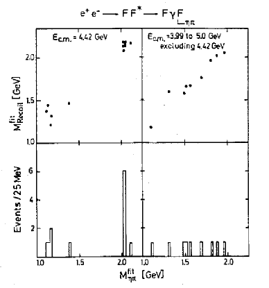
Figure 8: (Top) Fitted $\eta\pi^{\pm}$ mass versus fitted recoil mass assuming $e^{+}e^{-}\to FF^{*}$, where $F^{*}\to F\gamma$, and $F^{\pm}\eta\pi^{\pm}$ at (left) $E_{cm}$=4.42 GeV and (right) at all other energies excluding 4.42 GeV. At the bottom are the fitted $M(\eta\pi)$ projections.

The $F$ mass had an ambiguity because the low momentum photon from the $F^{*}$ decay could be associated either with the $F$ that decayed into $\eta\pi$ or with the $F$ that wasn’t reconstructed. Thus they found two possible mass values for the $F$, 2040$\pm$10 MeV or 2000$\pm$40 MeV. The generally quoted value was 2020-2030 MeV.

There was however a disturbing aspect of this result. The Crystal Ball group, operating at SPEAR checked the level of $\eta$ production in the same center-of-mass energy region.[21] A comparison of their result with the DASP result is shown in Fig. 9.

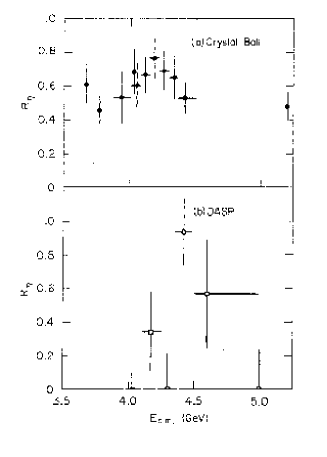
Figure 9: $R_{\eta}=\sigma(e^{+}e^{-}\to\eta X)/\sigma(e^{+}e^{-}\to\mu^{+}\mu^{-})$ for (a) Crystal Ball and (b) DASP.

Crystal Ball, which had a far superior ability to detect photons compared to DASP, did not find the increase in $\eta$ production at 4.42 GeV that DASP claimed. Without an increase in $\eta$ production it’s hard to see why $FF^{*}$ would be produced at 4.42 GeV and not at other energies. Unfortunately the Crystal Ball experiment did not have charged track momentum analysis and could not look for $F$’s.

In 1981 a group using the CERN Omega Spectrometer with a 20-70 GeV photon beam found evidence for the $F$ meson at 2020$\pm$10 MeV in several different decay modes. They used two sets of selection criteria to record data, denoted T1 and T2.[22] T1 required a minimum of four charged particles at a plane 1.5 m downstream of the target center. T2 required a photon with transverse momentum greater than 800 MeV and at least one charged track leaving the target. They show results for selected decay modes containing $\eta\to\gamma\gamma$ in Fig. 10.

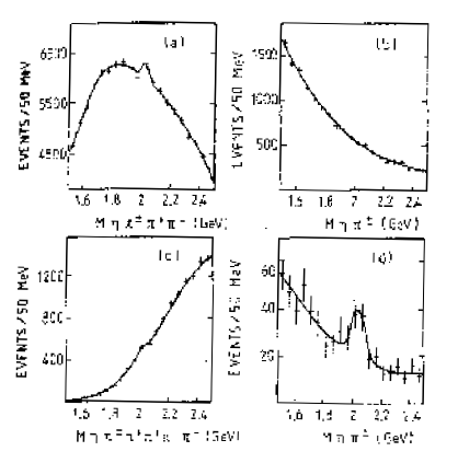
Figure 10: Mass spectra of (a) $\eta\pi^{\pm}\pi^{+}\pi^{-}$ from T1, (b) $\eta\pi^{\pm}$ from T1, (c) $\eta\pi^{\pm}\pi^{+}\pi^{-}\pi^{+}\pi^{-}$ from T1, and (d) $\eta\pi^{\pm}$ from T2. The curves are polynomial plus Breit-Wigner fits.

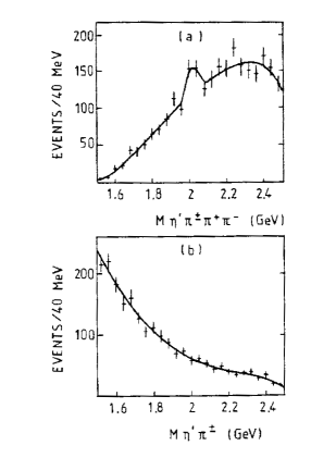
Figure 11: Mass spectra of (a) $\eta^{\prime}\pi^{+}\pi^{+}\pi^{-}$, a subset of (c) in Fig. 10, (b) $\eta\pi^{\pm}$, a subset of (a) in Fig. 11. The curves are polynomial plus Breit-Wigner fits.

In Fig. 11 they select candidates for $\eta^{\prime}\to\pi^{+}\pi^{-}\eta$ from the $\eta 5\pi$ and $\eta 3\pi$ samples. They see a signal in $\eta^{\prime}3\pi$ and nothing in $\eta^{\prime}\pi$.

In a 1983 paper they presented results based on a different trigger where they required one photon with energy greater than 2 GeV and forward charged multiplicity between 2 and 5.[23] Their data are shown in Fig. 12. The $F$ mass value was virtually unchanged.

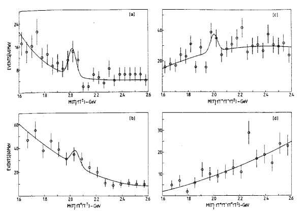
Figure 12: Mass spectra of $\eta(n\pi^{\pm})$ from the CERN Omega spectrometer. The curves are polynomial plus Gaussian fits.

These newer signals are quite weak, as was a signal they found in $\phi\rho^{\pm}$. They did not see a signal in $\phi\pi^{\pm}$.[24] For the $\phi$ results they used a different trigger that required between 4 and 9 charged tracks including an identified $K^{\pm}$, called T4. This group also published results on $D$ meson production.[25] The relevant yields are listed in Table 1.

Table 1: CERN Omega Spectrometer Photo-production Yields for $F$ Mesons into $\eta$, $\eta^{\prime}$ or $\phi$ and $D$ Modes into Kaons.

Mode	Trigger	Efficiency	# of events or significance	$\cal{B}\times\sigma$ (nb)
$\eta\pi^{+}\pi^{-}\pi^{\pm}$	T1	10	4$\sigma$	60$\pm$15
$\eta^{\prime}\pi^{+}\pi^{-}\pi^{\pm}$	T1	5	3$\sigma$	20$\pm$  8
$\eta\pi^{\pm}$	T2	3	5$\sigma$	27$\pm$  7
$\eta\pi^{\pm}$	T1	12		$<$45
$\eta^{\prime}\pi^{\pm}$	T1	6		$<$30
$\eta\pi^{\pm}$	T3	1.83	17$\pm$6	38$\pm$14
$\eta\pi^{\circ}\pi^{\pm}$	T3	0.85	14$\pm$9	66$\pm$42
$\eta\pi^{+}\pi^{-}\pi^{\pm}$	T3	0.87	20$\pm$11	93$\pm$52
$\phi\pi^{\pm}$	T4			$<$4
$\phi\rho^{\pm}$	T4		3$\sigma$	33$\pm$10
$\phi\pi^{+}\pi^{-}\pi^{\pm}$	T4			$<$15
$K^{-}\pi^{+}$		42	60$\pm$17	13.5$\pm$ 4
$K^{-}\pi^{+}\pi^{\circ}$		5	63$\pm$19	108$\pm$33
$K^{\circ}\pi^{+}\pi^{-}$		17	66$\pm$19	39$\pm$11
Efficiencies include $\eta^{(^{\prime})}$ decay fractions. Upper limits are at 3$\sigma$.

Now there are several significant problems here comparing $D^{\circ}$ production with $F^{\pm}$ production. First of all product of the branching ratio times production cross section ($\sigma\cdot\cal{B}$) for $F^{\pm}\to\eta\pi^{\pm}$ is more than twice as large as for $D^{\circ}\to K^{-}\pi^{+}$. It is expected that the $F$, being a charmed-strange meson, would be produced approximately 15% as often as the charmed-light quark combination. While the two-body branching ratios cannot be accurately predicted, the $\eta\pi$ would have to be about 14 times larger in the $F$ than the $K^{-}\pi^{+}$ was in the $D^{\circ}$. Since it was known that $K^{-}\pi^{+}$ was about 3%, this would have required a $\sim$40% branching ratio for $F\to\eta\pi$. Secondly, the production mechanism for $D$ decay had been shown to be mostly associated production, where $\gamma p\to\overline{D}\Lambda_{C}X$, while in the $F$ data the production was mostly $\gamma p\to F^{+}F^{-}X$. Why should the $F$ production mechanism be so different? In any case the accepted $F$ mass now was 2020$\pm$10 MeV, having now been “confirmed” by the CERN Omega data.

In July of 1980 one $F^{+}$ decay was detected in emulsion reactions from a neutrino beam, in the here-to-fore unknown decay mode $\pi^{+}\pi^{+}\pi^{-}\pi^{\circ}$. The mass was determined to be 2017$\pm$25 MeV, and lifetime of 1.4$\times 10^{-13}$s measured.[26] Later in Sept. of that year another neutrino emulsion experiment [27] measured a lifetime with two events.

In 1983 the CLEO experiment presented results that showed strong evidence for the $F$ at 1970$\pm$5$\pm$5 MeV. The evidence consisted of a mass peak containing 104$\pm$19 events in the $\phi\pi^{\pm}$ decay mode shown in Fig. 13, the helicity distribution of the $\phi$, that showed the expected $\cos^{2}\theta$ decay angular distribution and a $\sigma\cdot\cal{B}$ that was 1/3 of the $\sigma\cdot\cal{B}$ for $D^{\circ}\to K^{-}\pi^{+}$.[28] I can assure you that the CLEO collaboration was not easily persuaded by myself and Yuichi Kubota that our results were right because they contradicted the previous experiments shown above. We were forced to go through experiment by experiment and detail what might have gone wrong. (Thus the material for this section was created.) The CLEO result was quickly confirmed by TASSO,[29] ACCMOR,[30] and ARGUS experiments.[31] The Particle Data Group subsequently chose to rename the $F$ as the $D_{s}$, a logical choice.

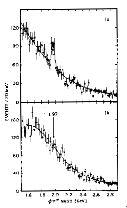
Figure 13: (a) Mass spectra of $\phi\pi^{\pm})$ from CLEO. (b) The $\phi$ candidates are chosen to be above or below the $\phi$ signal region.

What lessons are we to learn from this story? DASP based their “discovery” on the obervation of increased $\eta$ production at 4.42 GeV and a handful of events where one $F$ was reconstructed in $\eta\pi^{\pm}$ and the other not reconstructed. Presumably they searched many energies and several final states including $F^{+}F^{-}$ and $F^{*+}F^{*-}$, reporting a signal in only one case. However, the statistical significance is often viewed by not considering all the searches that yielded no signal.

The CERN Omega spectrometer results all were of very marginal accuracy and didn’t fit together very well. The $F$ production mechanism was completely different than that for $D$’s, the rates for $\eta\pi^{\pm}$ were more than 7 times larger than for $\phi\pi^{\pm}$, yet these discrepancies were never addressed. We note that none of their results for the relative branching ratios are consistent with current measurements.[32] For example, $\eta\pi^{\pm}$ is about half of $\phi\pi^{\pm}$ and $\phi\rho^{\pm}$ is twice $\phi\pi^{\pm}$. Apparently their data showed marginal signals at 2020 MeV and the DASP result was sufficient to push them over the edge in giving credibility to their fluctuations.

The neutrino experiments now had the DASP and CERN Omega results to fall back on. Doubtless if they hadn’t believed the 2020 MeV value for the mass they may not have shown their results; on the other hand, they could have been more conservative.

The DASP, Omega and neutrino results satisfy Langmuir’s first criterion: “The maximum effect that is observed is….of barely detectable intensity….” Even more so the second criterion is fully satisfied, especially by the Omega result: “The effect is of a magnitude that remains close to the limit of detectability, or many measurements are required because of the low statistical significance of the results.” The neutrino experiments satisfied his third criteria, “Claims of great accuracy,” in that they measured lifetimes! Criteria (4) and (5) did not come into play although (4) should have been invoked to explain production yields and relative branching ratios. Criterion (6), “Ratio of supporters to critics …” was funny in that most people believed the DASP and Omega results until the CLEO result came out and then suddenly no one believed them.

8 Conclusions

Be suspicious of new results. Think them over and if they don’t make sense then doubt them. It doesn’t mean they are wrong, just not proven. Sometimes it’s difficult to know when something is right or wrong.

It is also difficult to find out exactly what went wrong unless you are directly involved with an experiment or had the opportunity to visit and question as Langmuir had. Even Langmuir found it difficult to figure out the process. From Langmuir: “I don’t know what it is. That’s the kind of thing that happens in all these. All the people who had anything to do with these things find that when you’re through with them some things are inexplicable. You can’t account for Bergen Davis saying that they didn’t calculate those things from the Bohr theory, that they were found by empirical methods without any idea of the theory. Barnes made the experiments, brought them in to Davis, and Davis calculated them up and discovered all of a sudden that they fit the Bohr theory. He said Barnes didn’t have anything to do with that. Well, take it or leave it. How did he do it? It’s up to you to decide. I can’t account for it. All I know is that there was nothing salvaged at the end, and therefore none of it was ever right, and Barnes never did see a peak. You can’t have a thing halfway right.”

As a final note, Prof. Roodman at this school described how some current experiments, KTeV, Babar and Belle have ensured that the final answer to their most important measurements is actually hidden from the data analyzers until they are satisfied that all systematic checks have been performed.[33] In my view this is a useful technique and should be employed more often. Another method that has been employed is to have different groups within a collaboration obtain their results independently.

Hopefully reviewing these painful lesson will help others avoid the same pitfalls.

9 Acknowledgements

I would like to thank Tom Ferbel for showing me Langmuir’s paper long ago. Thanks to K. T. Mahanthappa, H. Murayama and J. Rosner for organizing a very interesting school and inviting me to participate. Ray Mountain and Jon Rosner helped greatly by carefully reading and editing this paper.

References

- [1] I. Langmuir, “Pathological Science,” General Electric, (Distribution Unit, Bldg. 5, Room 345, Research and Development Center, P. O. Box 8, Schenectady, NY 12301), 68-C-035 (1968).
- [2] A. H. Barnes, Phys. Rev. 35, 217 (1930).
- [3] B. Davis and A. H. Barnes Phys. Rev. 37, 1368 (1931).
- [4] R. Blondlot, The N-rays, Longmans, Green and Co., London, England (1905).
- [5] R. W. Wood, Nature, 72, 195 (1904); R. W. Wood, Physik. Z. 5, 789 (1904).
- [6] G. E. Chikovani et al., Phys. Lett. 25B, 44 (1967).
- [7] H. Benz et al, Phys. Lett. 28B, 233 (1968).
- [8] K. Böckman et al., Nucl. Phys. B 16, 221 (1970)
- [9] M. Anguilar-Benitez et al., Phys. Lett. B 29, 62 (1969)
- [10] D. J. Crennell et al., Phys. Rev. Lett. 20, 1318 (1968)
- [11] A. Barbaro-Galtieri, “The and the Nonet,” in Experimental Meson Spectroscopy, ed. C. Baltay and A. H. Rosenfeld, (Columbia Univ. Press, New York, 1970.
- [12] The LBL data were published in M. Alston-Garnjost et al., Phys. Lett. B 33, 607 (1970).
- [13] K. J. Foley et al., Phys. Rev. Lett. 36, 413 (1971); G. Grayer et al., Phys. Lett. B 34, 333 (1971).
- [14] D. Bowen et al., Phys. Rev. Lett. 26, 1663 (1971)
- [15] Experimental Meson Spectroscopy - 1972, ed. A. H. Rosenfeld and K. W. Lai, (American Institute of Physics, New York, 1972).
- [16] R. Baud et al.“Charged Non-strange Bosons with Masses Higher Than 2.5 GeV,” in Experimental Meson Spectroscopy, ed. C. Baltay and A. H. Rosenfeld, (Columbia Univ. Press, New York, 1970).
- [17] D. H. Miller, “Comparison of the CERN Boson Spectrometer Results with a Experiment at 13 GeV/c in a Bublle Chamber,” in Experimental Meson Spectroscopy, ed. C. Baltay and A. H. Rosenfeld, (Columbia Univ. Press, New York, 1970).
- [18] G. Kalbfleisch “The T Region,” in Experimental Meson Spectroscopy, ed. C. Baltay and A. H. Rosenfeld, (Columbia Univ. Press, New York, 1970).
- [19] A famous U. S. television show from the 1950’s, “Dragnet,” ended by saying “…the names were changed to protect the innocent.”
- [20] R. Brandelik et al., Phys. Lett. B 70, 132 (1977); ibid, Phys. Lett. B 67, 243 (1977); ibid Phys. Lett. B 34, 358 (1977); ibid, Phys. Lett. B 80, 412 (1979).
- [21] F. C. Porter, “Measurement of Inclusive Production in Interactions Near Charm Threshold,” in High Energy Physics-1980, XX Int. Conf. ed. L. Durand and L. Pondrom, American Institute of Physics, New York (1981) p380.
- [22] D. Aston et al., Phys. Lett. B 100, 91 (1981).
- [23] M. Atkinson et al., Z. Phys. C 17, 1 (1983).
- [24] D. Aston et al., Nucl. Phys. B 189, 205 (1981).
- [25] D. Aston et al., Phys. Lett. B 94, 113 (1980).
- [26] R. Ammar et al., Phys. Lett. B 100, 118 (1980).
- [27] N. Ushida et al., Phys. Rev. Lett. 45, 1053 (1980).
- [28] A. Chen et al., Phys. Rev. Lett. 51, 634 (1983).
- [29] M. Althoff et al., Phys. Lett. B 136, 130 (1984).
- [30] R. Bailey et al., Phys. Lett. B 139, 320 (1984).
- [31] H. Albrecht et al., Phys. Lett. B 146, 111 (1984); H. Albrecht et al., Phys. Lett. B 153, 343 (1984).
- [32] Particle Data Group, Eur. Phys. J. C15, 1 (2000).
- [33] A. Roodman, “Results from Asymmetrical Collisions,” in Theoretical Advanced Study Insitute In Elementary Particle Physics, Boulder, CO, June, 2000.