Electroweak phase transition
beyond the Standard Model

Abstract

Standard theories of electroweak interactions are based on the concept of a gauge symmetry broken by the Higgs mechanism. If they are placed in an environment with a sufficiently high temperature, the symmetry gets restored. It turns out that the characteristics of the symmetry restoring phase transition, such as its order, are important for cosmological applications, such as baryon asymmetry generation. We first briefly review how, by a combination of analytic and numerical methods, the properties of the phase transition can be systematically resolved for any given type of a (weakly interacting) Higgs sector. We then summarise the numerical results available for the Standard Model, and present a generic model independent statement as to how the Higgs sector should differ from the Standard Model for the properties of the transition to be very different. As an explicit example, we discuss the possibilities available for a strong transition in the experimentally allowed parameter region of the Minimal Supersymmetric Standard Model.

hep-ph/0010275

1 Introduction

Even though a Higgs particle remains to be discovered, the success of precision computations gives strong support to the idea of an SU(2)$\times$U(1) electroweak theory with one or more Higgs doublets, some of which have, in any practical gauge, a non-vanishing expectation value at zero temperature. However, when the theory is placed in an environment with a sufficiently high temperature, the symmetry generically gets restored. [1] Thus we may imagine that there was an electroweak phase transition in the Early Universe.

An outstanding physics motivation for these considerations was perceived about fifteen years ago. [2] Indeed, an electroweak phase transition might in principle leave as a remnant the matter–antimatter (baryon) asymmetry presently observed. An essential ingredient in this statement is that there are anomalous baryon number violating interactions which are fast enough to be in thermal equilibrium at temperatures above the transition. [2] If the transition is sufficiently strongly of the first order, i.e. discontinuous, baryon number violating interactions are however switched off below the transition temperature, in the broken phase. Together with the CP violation known to exist in nature, as well as the non-equilibrium dynamics always present in first order transitions, these ingredients might suffice to produce an asymmetry with the correct order of magnitude (for a review, see ref. [3]).

In the present talk, we will not enter any details of the actual baryogenesis computations, but simply consider the existence and strength of a first order phase transition. As a reference value, we however recall that the constraint of sufficient baryon violation switch-off after the transition can be related to the Higgs expectation value over temperature $v/T$ in, say, the Landau gauge, or gauge invariantly to an appropriately regularized value of $\langle\phi^{\dagger}\phi\rangle/T^{2}\approx v^{2}/(2T^{2})$, where $\phi$ is the Higgs doublet. In the case of several SU(2) Higgs doublets, the observable is correspondingly $\sum_{i}\langle\phi^{\dagger}_{i}\phi_{i}\rangle/T^{2}$. The numerical requirement, based on 1-loop saddle point computations (for a summary of their status and accuracy, see [4]) as well as on a non-perturbative evaluation, [5] is that the discontinuity in $v/T$ across the phase transition should exceed unity, $\Delta v/T\mathop{\raise 1.29167pt\hbox{$>$\kern-7.5pt\raise-4.73611pt\hbox{$\sim$}}}1.0$.

2 General formulation of the problem

Let us start by stating more generally the types of quantities that we may want to determine. The most basic characteristic of a finite temperature system is its partition function $Z(T,V)$, or the free energy density $f(T)$, where

$$Z(T,V)=e^{-\beta{Vf(T)}}={\rm Tr\,}e^{-\beta{H}}.$$ (1)

Here $H$ is the Hamiltonian, $\beta=T^{-1}$, and $V\to\infty$ is the volume. The points $T=T_{c}$ where $f(T)$ is non-analytic are phase transition points, and if $\left.f^{\prime}(T)\right|_{T\to T_{c}^{\pm}}$ is discontinuous, the transition is of the first order. This implies also that the energy density, $e(T)=-T^{2}d[T^{-1}f(T)]/dT$, is discontinuous. In addition to $f(T),e(T)$, we also want to determine, as discussed above, the value of a (suitably regularized) $\langle\phi^{\dagger}\phi\rangle(T)$, which is very strongly correlated with the rate of baryon number violation in the broken phase.

In perturbation theory, one does not usually address directly $f(T)$ or $\langle\phi^{\dagger}\phi\rangle$, but rather the effective potential $V(v,T)$ for the length of the Higgs field, $|\phi|=v/\sqrt{2}$. After gauge fixing, $V(v,T)$ can be defined for instance as the free energy density after the introduction of a constraint $\delta(v/\sqrt{2}-V^{-1}\int d^{3}x|\phi(x)|)$ in the path integral. In the thermodynamic limit, the value of $V(v,T)$ at the global minimum gives the actual free energy density, $f(T)$.

We may now recall that for all such “static” observables, it is straightforward to write down an “imaginary time” Euclidian path integral expression. Thus, in principle we only need to compute simple well-defined functional integrals, without any ambiguities related e.g. to Minkowski space.

3 Why is it non-trivial?

One may ask, why not simply trust $V(v,T)$ computed from the functional integral using perturbation theory? Indeed, such computations have been carried out up to resummed 2-loop level for the Standard Model (SM) [6, 7, 8], as well as for the MSSM [9]^-[15]. It turns out that at finite temperatures perturbative computations are not a priori reliable, however. We will meet circumstances below where even the order of the phase transition is wrong.

The reason for the breakdown is referred to as the infrared (IR) problem of finite temperature field theory. [16] It concerns “light” bosonic degrees of freedom, and can be understood as arising from expansion parameters of the type

$$g^{2}n_{b}(m)=\frac{g^{2}}{e^{m/T}-1}\stackrel{{\scriptstyle m\ll T}}{{\sim}}\frac{g^{2}T}{m},$$ (2)

where $n_{b}(m)$ is the Bose-Einstein distribution function, $g^{2}$ is a generic coupling constant, the SU(2) gauge coupling in particular, and $m$ some perturbative mass scale appearing in the propagators. Adding numerical factors from known contributions up to 3-loop order, the largest expansion parameter in the system can more concretely be estimated as [4]

$$\epsilon\approx\frac{g^{2}T}{\pi m}.$$ (3)

Thus, relatively “light” ($m\ll g^{2}T$) degrees of freedom interacting with the Higgses are a problem, and should be studied non-perturbatively. Such modes include, for instance, SU(2) gauge bosons near the symmetric phase.

In principle, a seemingly obvious way to study the system non-perturbatively is to carry out four-dimensional (4d) finite temperature lattice simulations. However, in the present context this turns out to be quite demanding. This is, first of all, because the coupling is weak, so that there are multiple length scales, $(2\pi T)^{-1},(gT)^{-1},(g^{2}T)^{-1}$, difficult to fit simultaneously on a finite lattice. The second problem is that only the bosonic sector of the theory can be studied anyway, since chiral fermions cannot be efficiently handled in practice. Nevertheless, leaving out the fermions, large scale efforts have been undertaken, complete with an extrapolation to the continuum limit ([17, 18] and references therein). The method we shall follow here is, however, different.

4 Dimensional reduction and 3d effective field theories

It turns out that all the problems mentioned above can be overcome in an economic and precise way by the method of finite temperature effective field theories (for reviews, see [19]). The basic idea of such an approach is to combine perturbation theory and simulations, in regions where they work best: one can integrate out massive modes perturbatively, which works well since the couplings are small, and then study the dynamics of the light modes non-perturbatively. In the first step, the original 4d theory reduces to a three-dimensional (3d) effective one. For studying the electroweak phase transition in a weakly coupled theory ($m_{H}\mathop{\raise 1.29167pt\hbox{$<$\kern-7.5pt\raise-4.73611pt\hbox{$\sim$}}}250$ GeV), this approach works with a practical accuracy at the percent level, both from the point of view of dimensional reduction, [17, 20, 21] as well as numerical simulations. [4, 22, 23, 24]

More concretely, the degrees of freedom integrated out [8, 20, 25, 26, 27] are all the heavy beyond-the-SM particles, as well as the non-zero Matsubara modes of the SM particles. This includes, in particular, all fermions. The effective masses of such modes are $m\mathop{\raise 1.29167pt\hbox{$>$\kern-7.5pt\raise-4.73611pt\hbox{$\sim$}}}\pi T$ so that there are no IR-problems but, according to Eq.(3), a small expansion parameter $\sim{g^{2}}/{\pi^{2}}$. The largest corrections are related to the top Yukawa coupling. After this step, the theory lives in 3d, since all non-zero Matsubara modes have been removed. A second step can also be taken: [8, 20, 25, 26] the zero components of the gauge fields get radiatively a mass $m\sim gT$. Thus there are again no IR-problems but, according to Eq. (3), a small expansion parameter $\sim{g}/{\pi}$.

We will not discuss the precise details of these integrations in any more detail here. For previous reviews, we refer to [19], and for explicit generic rules for the integrations, to [20]. For the logic behind the formal conjecture concerning the parametric accuracy obtained with the types of super-renormalizable effective theories discussed here (viz., ${\delta G}/{G}\sim{\cal O}(g^{3})$, where $G$ is a general non-vanishing bosonic Green’s function), we refer to [28].

5 Phase diagram for the Standard Model

After the heavy degrees of freedom have been integrated out perturbatively, one still has to deal with the non-perturbative bosonic scales $m\mathop{\raise 1.29167pt\hbox{$<$\kern-7.5pt\raise-4.73611pt\hbox{$\sim$}}}g^{2}T$. In the case of the Standard Model and many of its extensions, [20] the only infrared modes left are a single Higgs $\phi$ and the spatial SU(2) and U(1) gauge fields, with field strength tensors $F_{ij},B_{ij}$. The Lagrangian is

$${\cal L}_{\rm 3d} = {1\over 2}{\rm Tr\,}F_{ij}^{2}+{1\over 4}B_{ij}^{2}+(D_{i}\phi)^{\dagger}D_{i}\phi+m_{3}^{2}\phi^{\dagger}\phi+\lambda_{3}(\phi^{\dagger}\phi)^{2}.$$ (4)

All knowledge about the original modes with their physical zero temperature parameters, as well as about the temperature, is encoded in the expressions for the effective couplings $m_{3}^{2},\lambda_{3},g_{3}^{2},g_{3}^{\prime 2}$. Here $g_{3},g_{3}^{\prime}$ denote the SU(2) and U(1) gauge couplings.

To get a feeling for the properties of the effective theory in Eq. (4), let us first apply 1-loop perturbation theory. Ignoring the tiny corrections from $g_{3}^{\prime 2}/g_{3}^{2}$ for the moment and tuning $m_{3}^{2}$ to be on the phase transition line, we find a first order transition, with the discontinuity

$$\Delta\frac{v}{gT}=\frac{1}{8\pi}\frac{g_{3}^{2}}{\lambda_{3}}\biggl{[}1+{\cal O}(\frac{\lambda_{3}}{g_{3}^{2}})\biggr{]}.$$ (5)

(The ${\cal O}(\lambda_{3}/g_{3}^{2})$ corrections are in fact not analytic.) Using that in the SM,

$$\frac{\lambda_{3}}{g_{3}^{2}}\approx{1\over 8}\frac{m_{H}^{2}}{m_{W}^{2}}+{\cal O}\Bigl{(}\frac{g^{2}}{(4\pi)^{2}}\frac{m_{\mbox{\scriptsize top}}^{4}}{m_{W}^{4}}\Bigr{)},$$ (6)

and inspecting, say, $m_{W}(T)=gv/2$ in the broken phase, we however see from Eq. (3) that for large (realistic) Higgs masses $m_{H}>m_{W}$ an IR sensitive computation of the type in Eq. (5) cannot be trusted at all.

Fortunately, we do not need to rely on perturbation theory. The theory in Eq. (4) is ideally suited for lattice simulations. Due to the simplicity of the action and its low dimensionality, extrapolations to the infinite volume and continuum limits can be systematically carried out [29, 30, 31].

Figure 1: The phase diagram of the physical Standard Model. The blobs indicate simulation points (with errorbars), and the solid curve is a fit through them.

The results of such lattice simulations from refs. [22, 32, 33] are summarised in Fig. 1. There is a line of first order phase transitions, which however ends at a critical point, after which there is only a crossover. The ending of the transition is in qualitative contrast with the perturbative prediction in Eq. (5).

The endpoint location has been determined with great precision, and corresponds in physical units to $m_{H,c}=72.3(7)$ GeV, $T_{c}=109.2(8)$ GeV [33]. The errors here are statistical, remaining after continuum extrapolation. In case one would now not be a priori convinced about the accuracy of dimensional reduction at the percent level, we may note that a similar phase diagram exists also in the bosonic 4d SU(2)$+$Higgs theory, where also direct 4d simulations have been carried out. [17] While the statistical errors are slightly larger, the results agree completely with the results obtained after leaving out fermions from the dimensional reduction expressions, as well as changing $g^{2}$ to the larger value used in ref. [17]. A detailed comparison of the whole phase diagram has been carried out in ref. [21], with full agreement for $m_{H}\mathop{\raise 1.29167pt\hbox{$>$\kern-7.5pt\raise-4.73611pt\hbox{$\sim$}}}30$ GeV. Thus, we can really rely on the result in Fig. 1.

Let us now discuss the physical conclusions drawn from Fig. 1. As pointed out in the Introduction, for baryogenesis we need a first order phase transition, and even a strong one, $\Delta v/T\mathop{\raise 1.29167pt\hbox{$>$\kern-7.5pt\raise-4.73611pt\hbox{$\sim$}}}1$. We have learned that a first order transition only exists for $m_{H}<72$ GeV. Furthermore, it has in fact $\Delta v/T\mathop{\raise 1.29167pt\hbox{$<$\kern-7.5pt\raise-4.73611pt\hbox{$\sim$}}}1.0$ down to $m_{H}\sim 10$ GeV! [4, 6, 7] Thus, we observe that experimentally allowed Higgs masses $m_{H}\mathop{\raise 1.29167pt\hbox{$>$\kern-7.5pt\raise-4.73611pt\hbox{$\sim$}}}110$ GeV [34] are very far from allowing for a first order electroweak phase transition, let alone for electroweak baryogenesis.

Finally, let us briefly mention a related physics topic, which is of some interest because its solution is not yet understood as well as the issues above. It is the question as to how the properties of the phase transition change if there are primordial magnetic fields present, [35] or, more generally, whether magnetic fields could in some way be related to the baryon asymmetry. [36]

6 How to change the properties of the phase transition?

From the discussion in the previous section, it is clear that if we want to have an electroweak phase transition which is of the first order for realistic Higgs masses, and even strongly so, then a drastic change is needed with respect to the Standard Model.

What is it that should be changed? As the strength of the transition is determined by the scalar self-coupling, cf. Eq. (5), we apparently need some new degree of freedom which can decrease the effective $\lambda_{3}$ by ${\cal O}(100\%)$. To get such a large correction in the first place, we need a bosonic zero mode with an expansion parameter like in Eq. (3). A simple perturbative 1-loop computation shows that at least the sign of loop corrections of this type is the correct one, negative. But to have an effect of ${\cal O}(100\%)$, we need $\epsilon\sim 1$, so that $m\sim g^{2}T/\pi$. That is, the degree of freedom should itself be non-perturbative!

In principle, there are two kinds of possibilities for such degrees of freedom. Either it is a new type of a gauge field, maybe something like technicolour, or a scalar. In the latter, more natural case, there are thermal corrections in the effective mass parameter, appearing as $m_{3}^{2}\sim m_{\mbox{\scriptsize 4d}}^{2}+g^{2}T^{2}$. Thus, to get a total outcome of order $(g^{2}T)^{2}$, a cancellation must take place such that the mass parameter $m_{\mbox{\scriptsize 4d}}^{2}$ is negative. At zero temperature, the physical mass is then roughly $m_{\mbox{\scriptsize phys}}^{2}\mathop{\raise 1.29167pt\hbox{$<$\kern-7.5pt\raise-4.73611pt\hbox{$\sim$}}}m_{\mbox{\scriptsize 4d}}^{2}+m_{\mbox{\scriptsize top}}^{2}\mathop{\raise 1.29167pt\hbox{$<$\kern-7.5pt\raise-4.73611pt\hbox{$\sim$}}}m_{\mbox{\scriptsize top}}^{2}$. In order for such a relatively light degree of freedom not to have shown up so far in precision electroweak observables, it should be an SU(2) singlet.

It is interesting that scalar degrees of freedom satisfying these requirements can be found in realistic theories. Consider, for instance, the MSSM. Potential candidates are squarks and sleptons. Since they should couple relatively strongly to the Higgs, we should choose stops.

Now, the stops come left- and right-handed, $\tilde{t}_{L},\tilde{t}_{R}$ (these states can also mix, but for lack of space we ignore this here). The requirement of having a small violation of the electroweak precision observables means that the weakly interacting left-handed one cannot be light, $m_{\tilde{t}_{L}}\gg m_{\mbox{\scriptsize top}}$. This helps also in getting a large Higgs mass (see, e.g., ref. [37]),

$$m_{H}^{2}\sim m_{Z}^{2}\cos^{2}\!2\beta+\frac{3g^{2}}{8\pi^{2}}\frac{m_{\mbox{\scriptsize top}}^{4}}{m_{W}^{2}}\ln\frac{m_{\tilde{t}_{R}}m_{\tilde{t}_{L}}}{m_{\mbox{\scriptsize top}}^{2}}.$$ (7)

On the contrary, the SU(2) singlet stop $\tilde{t}_{R}$ can be “light”, and serve as the desired new degree of freedom. (Then we of course lose half of the correction to $m_{H}$ in Eq. (7), but this is the price to pay.) It should not be so light that the stop direction gets broken before the electroweak phase transition, though, because then one cannot get back to the SM minimum afterwards. [14]

Another example of a viable light scalar degree of freedom is the complex gauge singlet of the NMSSM, which can also get broken during the transition (for a recent study, see [38]).

7 Numerical results for the MSSM

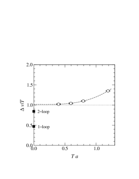
Figure 2: The continuum extrapolation (i.e., lattice spacing $a\to 0$) of the numerically determined $\Delta v/T$, compared with perturbation theory, for particular MSSM parameters. [39] The transition is strongly of the first order here.

Under the conditions described in the previous section, resummed 2-loop perturbation theory indicates that the electroweak phase transition can indeed be strong enough for baryogenesis. [10]^-[15] To check the reliability of perturbation theory, a 3d effective theory was constructed in refs. [10, 40]. The Lagrangian in Eq. (4) is supplemented by the right-handed stop field $U$ and the SU(3) gauge fields, with the field strength tensor $G_{ij}$:

$$\delta{\cal L}_{\mbox{\scriptsize 3d}}={1\over 2}{\rm Tr\,}G_{ij}^{2}+(D_{i}^{s}U)^{\dagger}D_{i}^{s}U+m_{U3}^{2}U^{\dagger}U+\lambda_{U3}(U^{\dagger}U)^{2}+\gamma_{3}\phi^{\dagger}\phi U^{\dagger}U.$$ (8)

Simulations with this action have been carried out in ref. [41], and with a more complicated version thereof, involving two Higgs doublets, in ref. [39].

The results are illustrated in Fig. 2 for a particular choice of parameters. We find the encouraging outcome that, in fact, for a light right-handed stop the 2-loop estimates are reliable and even somewhat conservative. This is in strong contrast to the case of the SM at realistic Higgs masses.

Next, we must ask more rigorously whether this parameter region is indeed in agreement with all experimental data. The most important constraint comes from the lower bound on the Higgs mass. [34] There is a parameter in the MSSM, $m_{A}$, which determines whether the Higgs sector resembles that in the Standard Model ($m_{A}\mathop{\raise 1.29167pt\hbox{$>$\kern-7.5pt\raise-4.73611pt\hbox{$\sim$}}}120$ GeV) or not ($m_{A}\mathop{\raise 1.29167pt\hbox{$<$\kern-7.5pt\raise-4.73611pt\hbox{$\sim$}}}120$ GeV). In the latter case, the experimental lower bound is relaxed, [34] and since the transition needs not always get significantly weaker (see Fig. 3, and ref. [39] for more details), this case is acceptable. The other possibility is having a large $m_{A}$, but then the left-handed stop should be quite heavy, $m_{\tilde{t}_{L}}\mathop{\raise 1.29167pt\hbox{$>$\kern-7.5pt\raise-4.73611pt\hbox{$\sim$}}}2$ TeV (see Fig. 3), in order to increase the Higgs mass.

         

Figure 3: The Higgs mass $m_{H}$, and the maximal discontinuity $\Delta v/T$ according to 2-loop perturbation theory, as a function of $m_{A}$ (left) and $m_{\tilde{t}_{L}}$ (right). [39] With lines we indicate the regions least constrained by experiment (already somewhat smaller than in ref. [34]).

8 CP violation in the background field configuration

So far, we have discussed the strength of the phase transition. Let us finally very briefly touch another issue relevant for baryogenesis, CP violation.

Even though the strength of the phase transition is determined by a single “dynamical” Higgs doublet, in the MSSM there are of course in principle two of them, of which the one discussed above, $\phi$ in Eqs. (4), (8), was a particular linear combination (see, e.g., ref. [39]). However, the direction orthogonal to $\phi$ could play a role for CP violation. Indeed, when there are two Higgses, $H_{1},\tilde{H}_{2}$, then there is for instance a new low-dimensional gauge invariant CP-odd observable $\mathop{\rm Im}H_{1}^{\dagger}\tilde{H}_{2}$. It could obtain a non-vanishing value, in principle even a large one, as is the case in spontaneous CP violation. [42] If so, then at the semi-classical level, fermion mass matrices may obtain non-trivial space-dependent phases, so that particles and anti-particles have different dispersion relations, which could be of relevance to baryon asymmetry generation.

However, in practice such interesting effects are quite small. The reason is that all the effects related to the orthogonal direction are suppressed at least by $\sim g^{2}T/[\pi(m_{A}^{2}+0.5T^{2})^{{1\over 2}}]$.[39] Here $m_{A}$, experimentally $\mathop{\raise 1.29167pt\hbox{$>$\kern-7.5pt\raise-4.73611pt\hbox{$\sim$}}}m_{Z}$, [34] measures the deviation from the single Higgs doublet dynamics at zero temperature, and the temperature correction is seen to increase the suppression further on.

         

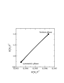
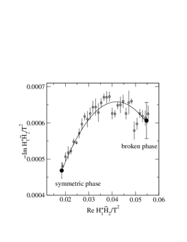
Figure 4: Behaviour of $H_{2}^{\dagger}H_{2}$, plotted against $H_{1}^{\dagger}H_{1}$, and $-\mathop{\rm Im}H_{1}^{\dagger}\tilde{H}_{2}$, plotted against $\mathop{\rm Re}H_{1}^{\dagger}\tilde{H}_{2}$, across a phase interface at $T_{c}$, for particular MSSM parameters. [39]

This situation is illustrated in Fig. 4, which shows the profile of a stationary phase interface (for perturbative analyses of such objects, see ref. [43] and references therein). We observe that in field space, the transition takes place in one particular direction (see also [18]), and CP violation is small, as if the system effectively only had one dynamical CP even Higgs doublet.

9 Conclusions

We have reviewed the methods that can be employed in determining the thermodynamical properties of the phase transition related to electroweak gauge symmetry restoration, as well as the numerical results that are already available for the Standard Model and for its Minimal Supersymmetric extension. The general statement to be remembered, is that there is no phase transition at all in electroweak theories with realistic Higgs masses, unless there is also another light scalar degree of freedom available, which plays an essential role in the phase transition dynamics.

As a concrete phenomenological example, we have recalled that it is still possible to find parts of the MSSM parameter space, not excluded by experiment, where the electroweak phase transition is strongly enough of the first order to allow for baryon asymmetry generation. However, these parts are quite restricted: not only does one need one “light” stop, $m_{\tilde{t}_{R}}\mathop{\raise 1.29167pt\hbox{$<$\kern-7.5pt\raise-4.73611pt\hbox{$\sim$}}}m_{\mbox{\scriptsize top}}$, in order to get a strong transition, but also either another stop which is much heavier, $m_{\tilde{t}_{L}}\mathop{\raise 1.29167pt\hbox{$>$\kern-7.5pt\raise-4.73611pt\hbox{$\sim$}}}10\,m_{\mbox{\scriptsize top}}$, or a Higgs sector which has at least two independent light particles, $m_{A}\mathop{\raise 1.29167pt\hbox{$<$\kern-7.5pt\raise-4.73611pt\hbox{$\sim$}}}120$ GeV, in order not to violate experimental constraints.

References

- [1] D.A. Kirzhnits, JETP Lett. 15, 529 (1972); D.A. Kirzhnits, A.D. Linde, Phys. Lett. B 42, 471 (1972); S. Weinberg, Phys. Rev. D 9, 3357 (1974); L. Dolan, R. Jackiw, Phys. Rev. D 9, 3320 (1974).
- [2] V.A. Kuzmin, V.A. Rubakov, M.E. Shaposhnikov, Phys. Lett. B 155, 36 (1985); M.E. Shaposhnikov, Nucl. Phys. B 287, 757 (1987).
- [3] V.A. Rubakov, M.E. Shaposhnikov, Usp. Fiz. Nauk 166, 493 (1996) [hep-ph/9603208].
- [4] K. Kajantie et al, Nucl. Phys. B 466, 189 (1996) [hep-lat/9510020].
- [5] G.D. Moore, Phys. Rev. D 59, 014503 (1999) [hep-ph/9805264].
- [6] P. Arnold, O. Espinosa, Phys. Rev. D 47, 3546 (1993) [hep-ph/9212235]; ibid. D 50, 6662 (1994) (E).
- [7] Z. Fodor, A. Hebecker, Nucl. Phys. B 432, 127 (1994) [hep-ph/9403219].
- [8] K. Farakos et al, Nucl. Phys. B 425, 67 (1994) [hep-ph/9404201].
- [9] J.R. Espinosa, Nucl. Phys. B 475, 273 (1996) [hep-ph/9604320]; B. de Carlos, J.R. Espinosa, Nucl. Phys. B 503, 24 (1997) [hep-ph/9703212].
- [10] D. Bödeker et al, Nucl. Phys. B 497, 387 (1997) [hep-ph/9612364].
- [11] M. Carena et al, Nucl. Phys. B 524, 3 (1998) [hep-ph/9710401].
-
[12]
J.M. Cline, G.D. Moore,
Phys. Rev. Lett. 81, 3315 (1998)
[hep-ph/
9806354]. - [13] M. Losada, Nucl. Phys. B 537, 3 (1999) [hep-ph/9806519].
- [14] J.M. Cline et al, Phys. Rev. D 60, 105035 (1999) [hep-ph/9902220].
- [15] M. Losada, Nucl. Phys. B 569, 125 (2000) [hep-ph/9905441]; S. Davidson, T. Falk, M. Losada, Phys. Lett. B 463, 214 (1999) [hep-ph/9907365].
- [16] A.D. Linde, Phys. Lett. B 96, 289 (1980); D.J. Gross, R.D. Pisarski, L.G. Yaffe, Rev. Mod. Phys. 53, 43 (1981).
- [17] F. Csikor et al, Phys. Rev. Lett. 82, 21 (1999) [hep-ph/9809291].
- [18] F. Csikor et al, Phys. Rev. Lett. 85, 932 (2000) [hep-ph/0001087].
- [19] M.E. Shaposhnikov, in Erice 1996, Effective theories and fundamental interactions, pp. 360–383 [hep-ph/9610247]; A. Nieto, Int. J. Mod. Phys. A 12, 1431 (1997) [hep-ph/9612291]; M. Laine, in Eger 1997, Strong and electroweak matter ’97, pp. 160–177 [hep-ph/9707415].
- [20] K. Kajantie et al, Nucl. Phys. B 458, 90 (1996) [hep-ph/9508379].
- [21] M. Laine, JHEP 9906, 020 (1999) [hep-ph/9903513].
- [22] K. Kajantie et al, Nucl. Phys. B 493, 413 (1997) [hep-lat/9612006].
- [23] O. Philipsen et al, Nucl. Phys. B 469, 445 (1996) [hep-lat/9602006].
- [24] M. Gürtler et al, Phys. Rev. D 56, 3888 (1997) [hep-lat/9704013].
- [25] A. Jakovác, A. Patkós, Phys. Lett. B 334, 391 (1994) [hep-ph/9405424]; Nucl. Phys. B 494, 54 (1997) [hep-ph/9609364].
- [26] J.M. Cline, K. Kainulainen, Nucl. Phys. B 482, 73 (1996) [hep-ph/9605235]; ibid. 510, 88 (1998) [hep-ph/9705201]; M. Losada, Phys. Rev. D 56, 2893 (1997) [hep-ph/9605266]; G.R. Farrar, M. Losada, Phys. Lett. B 406, 60 (1997) [hep-ph/9612346]; M. Laine, Nucl. Phys. B 481, 43 (1996) [hep-ph/9605283]; ibid. 548, 637 (1999) (E).
- [27] M. Laine, M. Losada, Nucl. Phys. B 582, 277 (2000) [hep-ph/0003111].
- [28] K. Kajantie et al, Phys. Lett. B 423, 137 (1998) [hep-ph/9710538].
- [29] K. Farakos et al, Nucl. Phys. B 442, 317 (1995) [hep-lat/9412091].
- [30] M. Laine, Nucl. Phys. B 451, 484 (1995) [hep-lat/9504001]; M. Laine, A. Rajantie, Nucl. Phys. B 513, 471 (1998) [hep-lat/9705003].
- [31] G.D. Moore, Nucl. Phys. B 493, 439 (1997) [hep-lat/9610013]; ibid. 523, 569 (1998) [hep-lat/9709053].
- [32] K. Rummukainen et al, Nucl. Phys. B 532, 283 (1998) [hep-lat/9805013].
- [33] M. Laine, K. Rummukainen, Nucl. Phys. B (Proc. Suppl.) 73, 180 (1999) [hep-lat/9809045].
-
[34]
ALEPH, DELPHI, L3, OPAL Collaborations,
http://alephwww.cern.ch/ALPUB/oldconf/oldconf00/29/moriond.ps. - [35] P. Elmfors et al, Phys. Lett. B 440, 269 (1998) [hep-ph/9806403]; K. Kajantie et al, Nucl. Phys. B 544, 357 (1999) [hep-lat/9809004]; M. Laine, hep-ph/0001292.
- [36] M. Joyce, M. Shaposhnikov, Phys. Rev. Lett. 79, 1193 (1997) [astro-ph/9703005]; M. Giovannini, M.E. Shaposhnikov, Phys. Rev. D 57, 2186 (1998) [hep-ph/9710234]; D. Comelli et al, Phys. Lett. B 458, 304 (1999) [hep-ph/9903227]; M. Laine, M. Shaposhnikov, Phys. Lett. B 463, 280 (1999) [hep-th/9907194].
- [37] J. Ellis, G. Ridolfi, F. Zwirner, Phys. Lett. B 262, 477 (1991).
- [38] S.J. Huber, M.G. Schmidt, Eur. Phys. J. C 10, 473 (1999) [hep-ph/9809506]; hep-ph/0003122.
- [39] M. Laine, K. Rummukainen, hep-lat/0009025.
- [40] M. Laine, K. Rummukainen, Nucl. Phys. B 545, 141 (1999) [hep-ph/9811369].
- [41] M. Laine, K. Rummukainen, Phys. Rev. Lett. 80, 5259 (1998) [hep-ph/9804255]; Nucl. Phys. B 535, 423 (1998) [hep-lat/9804019].
- [42] T.D. Lee, Phys. Rev. D 8, 1226 (1973).
- [43] S.J. Huber et al, Phys. Lett. B 475, 104 (2000) [hep-ph/9912278].