I Introduction

The possibility that at large quark densities the ground state of QCD is in a colour superconducting phase [1] has attracted much attention recently (see e.g. [2, 3] for recent reviews). The pattern of symmetry breaking is most interesting for three light quark flavours. Alford, Rajagopal and Wilczek [4] have shown that the diquark condensates lock the colour and flavour symmetry transformations: in the chiral limit, this colour-flavour locking (CFL) condensate spontaneously breaks both colour and flavour symmetries $SU(3)_{c}\times SU(3)_{L}\times SU(3)_{R}\times U(1)_{B}\rightarrow SU(3)_{c+L+R}$. Nine Goldstone modes survive to the Higgs mechanism.  One is a singlet, scalar mode, associated with the breaking of $U(1)_{B}$. The other eight Goldstone bosons belong to an octet of pseudoscalar modes associated with $SU(3)_{L}\times SU(3)_{R}$ chiral symmetry breaking, just like in vacuum. At low energies, $E\ll\Delta$ where $\Delta$ is the gap, an effective lagrangian and chiral perturbation theory ($\chi$PT) [5] can be used to study the dynamics of these light modes. Moreover, because of asymptotic freedom, at very large densities one can match the predictions of the effective theory with those of the underlying microscopic theory.

There has been already quite some work on the effective theory approach [6, 7, 8, 9, 10, 11, 12]. In the present letter we will be concern with the application of sum rules in the CFL phase. In particular, we will derive the expression for the pion decay constant as a direct consequence of chiral symmetry breaking. Although our result is not new, the formulation in term of sum rules is more general and also provides a self-consistent check of previous results. We also estimate the effects of chiral symmetry breaking by electromagnetic interactions.

II Weinberg sum rules in the CFL phase of QCD

We follow Casualboni and Gatto to construct the effective lagrangian [6]. With the diquark condensates defined as $X\sim\langle\psi_{L}\psi_{L}\rangle$ and $Y\sim\langle\psi_{R}\psi_{R}\rangle$, the low energy lagrangian in the chiral limit is 

$${\cal L} = {\cal L}_{V}+{\cal L}_{A}$$ (1)

$$= \frac{f^{2}_{\pi}}{4}\,\left({\rm Tr}\left(X\partial_{0}X^{\dagger}-Y\partial_{0}Y^{\dagger}\right)^{2}-v_{\pi}^{2}{\rm Tr}\left(X\partial_{i}X^{\dagger}-Y\partial_{i}Y^{\dagger}\right)^{2}\right)$$ (2)

$$+ \frac{af^{2}_{\pi}}{4}\,\left({\rm Tr}\left(X\partial_{0}X^{\dagger}+Y\partial_{0}Y^{\dagger}+2igG_{0}^{a}\frac{\lambda^{a}}{2}\right)^{2}-bv^{2}_{\pi}{\rm Tr}\left(X\partial_{i}X^{\dagger}+Y\partial_{i}Y^{\dagger}+2igG_{i}^{a}\frac{\lambda^{a}}{2}\right)^{2}\right)$$ (3)

where $G^{a}_{\mu}$ is the gluon field and $g$ is the gauge coupling constant. Defining the colour singlet matrix $\Sigma=XY^{\dagger}$, the first term in Eq. (1) becomes

$${\cal L}_{V}=\frac{f_{\pi}^{2}}{4}\left({\rm Tr}\left(\partial_{0}\Sigma\partial_{0}\Sigma^{\dagger}\right)-v^{2}_{\pi}{\rm Tr}\left(\partial_{i}\Sigma\partial_{i}\Sigma^{\dagger}\right)\right)\ .$$ (4)

The second term in Eq. (1) contains a mass term for the gluons. Since the gluons are heavy they can be integrated out and, to leading order at low energy, the effective lagrangian reduces to Eq. (4). Except for the breaking of Lorentz symmetry, the lagrangian (1) corresponds to the hidden gauge symmetry version of QCD in vacuum[13]. In that case, the vector mesons play the role of the gauge fields associated with the hidden gauge symmetry [13].

In Eq. (1) there are four independent parameters, $f_{\pi}$, $v_{\pi}$, $a$ and $b$. These parameters can be computed from the microscopic theory. The Debye and Meissner masses from Eq. (1) are given respectively by $m_{D}^{2}=ag^{2}f^{2}_{\pi}$ and $m^{2}_{M}=bv^{2}_{\pi}m^{2}_{D}$. These have been first computed by Son and Stephanov [7] from the microscopic theory and matched to those of the effective theory to derive

$$f_{\pi}^{2}={21-8\ln{2}\over 18}\,{\mu^{2}\over 2\pi^{2}}\ ,\qquad v_{\pi}=\frac{1}{\sqrt{3}}\,.$$ (5)

They also argued that $a=b=1$ to leading order in the gauge coupling, because those values could be only modified by higher loop effects. Although their conclusion is correct, the argument has a potential flaw. We will see that, because of infrared divergences in the CFL phase of QCD, the connection between the loop and gauge coupling expansions is lost. For instance, it is not a priori guaranteed that a two-loop diagram is suppressed with respect to a one-loop diagram at weak coupling.

In this letter we present an alternative derivation of $f_{\pi}$, which turns into a consistency check of the results in Eq. (5). Our computation relies on defining $f_{\pi}$ as the constant which parametrises the asymmetry between two-point vector and axial-vector correlators in the ground state of the CFL phase. Since Lorentz symmetry is broken there are two possible independent correlators which can be defined. If $V^{a}_{\mu}={\bar{\psi}}\gamma^{\mu}\frac{\lambda^{a}}{2}\psi$ and $A^{a}_{\mu}={\bar{\psi}}\gamma^{\mu}\gamma_{5}\frac{\lambda^{a}}{2}\psi$ are the vector and axial-vector flavour currents, respectively, then in the chiral limit $m_{q}=0$,

$$f^{2}_{\pi}\delta^{ab} = i\int d^{4}x\,\left\{\langle V_{0}^{a}(x)V_{0}^{b}(0)\rangle-\langle A_{0}^{a}(x)A_{0}^{b}(0)\rangle\right\}\ ,$$ (7)

$$-v^{2}_{\pi}f^{2}_{\pi}\delta^{ab} = i\int d^{4}x\,\left\{\langle V_{i}^{a}(x)V_{i}^{b}(0)\rangle-\langle A_{i}^{a}(x)A_{i}^{b}(0)\rangle\right\}\ .$$ (8)

These relations can be inferred from the fact that the axial-vector currents taken between the ground state and a pion state give [14] (see appendix B)

$$\langle 0|A_{a}^{0}|\pi^{b}(p)\rangle=if_{\pi}\delta^{ab}p^{0}\ ,\qquad\langle 0|A_{a}^{i}|\pi^{b}(p)\rangle=iv^{2}_{\pi}f_{\pi}\delta^{ab}p^{i}\ .$$ (9)

Prior to the discovery of QCD, Weinberg [15] derived a set of relations between the moments of the spectral functions of vector and axial-vector currents in vacuum (see e.g. [16] for a review). If one writes the correlators of vector and axial-vector currents in terms of their spectral densities, we could generalise the Weinberg sum rule [15] to the CFL phase. We will not write explicitly these relations here, but just note that they are directly deduced from Eqs. (II).

From Eqs. (II) one sees that $f_{\pi}$ is the order parameter for spontaneous chiral symmetry breaking. If we compute the Debye mass independently and take the ratio between $m^{2}_{D}/g^{2}f^{2}_{\pi}$, we get $a$. Similarly, the constant $b$ is computed as the ratio $m^{2}_{M}/m_{D}^{2}v^{2}_{\pi}$. Note that in the hidden symmetry approach to vector mesons, the value $a=2$ allows to implement vector meson dominance in the chiral lagrangian [13].

We will first review the computation of the Debye and Meissner masses. This computation has been done by several authors [7, 17] but, for completeness, we repeat it here using the natural quark basis for the CFL phase. The Nambu-Gorkov quark propagators are diagonal in the colour-flavour basis while the Feynman rules for the vertices are non-diagonal (appendix A). To compute the Debye and Meissner masses, one evaluates the gluon polarization tensor as in Fig.1,

$$\Pi^{\mu\nu}_{ab}(k) = -i\frac{g^{2}}{32}\sum_{B,C=1}^{9}{\rm Tr}\left(\lambda^{B}\lambda^{a}\lambda^{C}\right){\rm Tr}\left(\lambda^{C}\lambda^{b}\lambda^{B}\right)I_{BC}^{\mu\nu}(k)$$ (10)

$$+ i\frac{g^{2}}{32}\sum_{B,C=1}^{9}{\rm Tr}\left(\lambda^{B}\lambda^{a}\lambda^{C}\right){\rm Tr}\left(\lambda^{B}\lambda^{b}\lambda^{C}\right)R_{BC}^{\mu\nu}(k)\ ,$$ (11)

where

$$I_{BC}^{\mu\nu}(k) = \sum_{e=\pm}\int\frac{d^{4}q}{(2\pi)^{4}}{\rm Tr}\left(\gamma^{\mu}S^{e}_{C}(q)\gamma^{\nu}S_{B}^{e}(q-k)\right)\ ,$$ (13)

$$R_{BC}^{\mu\nu}(k) = \sum_{e=\pm}\int\frac{d^{4}q}{(2\pi)^{4}}{\rm Tr}\left(\gamma^{\mu}\Xi^{e}_{C}(q)\gamma^{\nu}\Xi_{B}^{-e}(q-k)\right)\ ,$$ (14)

and $S_{A}^{\pm}/\Xi^{\pm}_{A}$ are the diagonal/off-diagonal terms in the Nambu-Gorkov matrix propagator (see Appendix A).

The calculation of Eq. (10) gets simpler by realizing that the quark propagators $S^{\pm}_{A}$ and $\Xi^{\pm}_{A}$ are the same for all the values of $A$, except $A=9$. The $U(3)$ traces of Eq. (10) can then be easily evaluated. To compute the Debye and Meissner masses, it is enough to evaluate the polarisation tensor at $k=0$,

$$\Pi_{ab}^{00}(k=0) = -i\frac{g^{2}}{12}\delta_{ab}\left[7I_{11}^{t}(k=0)+2I^{t}_{19}(k=0)+2R^{t}_{11}(k=0)-2R^{t}_{19}(k=0)\right]\ ,$$ (15)

$$\Pi_{ab}^{ij}(k=0) = -i\frac{g^{2}}{12}\delta^{ij}\delta_{ab}\left[7I_{11}^{s}(k=0)+2I^{s}_{19}(k=0)+2R^{s}_{11}(k=0)-2R^{s}_{19}(k=0)\right]\ .$$ (16)

The superscript $t$ and $s$ above refers to, respectively, the purely temporal and purely spatial components of the tensors defined in Eqs. (II). In the static limit, $I^{0i}_{AB}=R^{0i}_{AB}=0$, thus $\Pi^{0i}_{ab}(k=0)=0$. An explicit computation of the integrals in Eqs. (II) gives, to leading order,

$$I^{t}_{11}(k=0) = I^{t}_{19}(k=0)=2i\frac{\mu^{2}}{2\pi^{2}}\ ,$$ (18)

$$R^{t}_{11}(k=0) = -2i\frac{\mu^{2}}{2\pi^{2}}\ ,\qquad R^{t}_{19}(k=0)=i\frac{8}{3}\ln{2}\,\frac{\mu^{2}}{2\pi^{2}}\ ,$$ (19)

$$I^{s}_{11}(k=0) = I^{s}_{19}(k=0)=-\frac{2}{3}i\frac{\mu^{2}}{2\pi^{2}}\ ,$$ (20)

$$R^{s}_{11}(k=0) = -\frac{1}{3}R^{t}_{11}(k=0)\ ,\qquad R^{s}_{19}(k=0)=-\frac{1}{3}R^{t}_{19}(k=0)\ .$$ (21)

It is maybe worth noticing that in the static limit the integrals in Eqs. (II) for the temporal components are dominated by quark-quark excitations. The antiquark-antiquark contribution is suppressed and can be neglected. Also the contribution of quark-antiquark excitations is precisely vanishing. However, for the spatial components, the quark-antiquark excitations do contribute to $I^{s}_{11/19}(k=0)$. This fact has already been stressed in [17]. The Debye and Meissner masses are finally given by

$$m_{D}^{2}=g^{2}\,{21-8\ln{2}\over 18}\,{\mu^{2}\over 2\pi^{2}}\ ,\qquad m_{M}^{2}=\frac{1}{3}\,m_{D}^{2}\ ,$$ (22)

expressions which agree with the results of [7, 17].

We now turn to the evaluation of the correlators of vector and axial-vector currents in QCD. The best strategy to compute them is to define the generating functional $Z$ for the Green’s functions of vector and axial-vector quark currents in presence of external sources $v_{\mu}$ and $a_{\mu}$

$$e^{iZ[v,a]}=\langle T\exp{\left(i\int dx\,{\bar{\psi}}\gamma_{\mu}\left(v^{\mu}+\gamma_{5}a^{\mu}\right)\psi\right)}\rangle\ .$$ (23)

Then functional derivatives of $Z$ with respect to the sources evaluated at $v=a=0$ generate the desired correlators.

Now we face a little puzzle. Since the leading order expression for $f_{\pi}^{2}$ as computed by Son and Stephanov does not depend on $g$, one would naively expect that the sum rule Eq. (II) is saturated by one-loop diagrams, i.e. with no gluon lines, as in Fig.2. However, due to the Dirac structure of the Nambu-Gorkov propagator, it is easy to verify that at this order, the r.h.s. of Eq. (II) is precisely zero ! But the next-to-leading order contribution is a priori ${\cal O}(g^{2})$, which seems to contradict the fact that $f_{\pi}^{2}$ is ${\cal O}(g^{0})$. Actually, this naive power counting is spoiled by infrared divergences and we will see that the next-to-leading order contribution is indeed independent of the gauge coupling.

The first non-vanishing contribution to the r.h.s. of Eq. (II) actually arises solely from the two-loop diagram depicted in Fig.3. Although it is naively of order $g^{2}$, it is easy to see that this dependence precisely cancels. The diagram is infrared divergent $\propto 1/k^{2}$ because of the gluon pole. But in the CFL phase and in the limit of zero external momentum, the gluon pole is trivially regulated by either the Debye or the Meissner mass. In both case, $1/k^{2}\rightarrow 1/g^{2}\mu^{2}$. Taking into account the factor of $g^{2}$ from the gluon vertices, we conclude that the diagram is ${\cal O}(g^{0})$, as desired. There are other diagrams with the same topology but they do not contribute. First, if we replace an external vector current by an axial-vector one, the diagram vanishes because of the trace over $\gamma_{5}$. Furthermore, we will see below that the diagrams with normal quark propagators (i.e. diagonal components of the Nambu-Gorkov matrix of propagators) do also vanish.

We evaluate the diagram of Fig.3 by computing each quark loop separately. In each of them, there is both a gluon vertex and a flavour vector current vertex. The computation is superficially the same as for the one-loop polarisation tensor (10). The important difference is that the Feynman rules for these two vertices are different because the gluon vertex changes colour but leave the flavour indices untouched, while the flavour vector current vertex does the opposite. This is clearly reflected in the Feynman rules in the CFL basis given in Appendix A. For each loop we find

$$\frac{g}{32}\ \sum_{B,C=1}^{9}{\rm Tr}\left(\lambda^{B}\lambda^{a}\lambda^{C}\right){\rm Tr}\left(\lambda^{C}\lambda^{b}\lambda^{B}\right)R_{BC}^{\mu\nu}(k)$$ (24)

which we evaluate in the limit $k\rightarrow 0$. We find

$$\delta_{ab} \frac{g}{12}\left(7R^{t}_{11}(k=0)+2R^{t}_{19}(k=0)\right)=-i\delta_{ab}\frac{m^{2}_{D}}{g}\ ,$$ (26)

$$\delta_{ab} \delta^{ij}\frac{g}{12}\left(7R^{s}_{11}(k=0)+2R^{s}_{19}(k=0)\right)=-i\delta_{ab}\delta^{ij}\frac{m^{2}_{M}}{g}\ ,$$ (27)

where we have used the results obtained in Eqs. (II). A similar one-loop diagram with the diagonal terms of the Nambu-Gorkov propagator gives

$$-\frac{g}{32}\sum_{B,C=1}^{9}{\rm Tr}\left(\lambda^{B}\lambda^{a}\lambda^{C}\right){\rm Tr}\left(\lambda^{B}\lambda^{b}\lambda^{C}\right)I_{BC}^{\mu\nu}(k)\ ,$$ (28)

which in the $k\rightarrow 0$ limit reduces to

$$\delta_{ab} \frac{g}{12}\left(2I^{t}_{11}(k=0)-2I^{t}_{19}(k=0)\right)=0\ ,$$ (30)

$$\delta_{ab} \delta^{ij}\frac{g}{12}\left(2I^{s}_{11}(k=0)-2I^{s}_{19}(k=0)\right)=0\ ,$$ (31)

so that it vanishes, as we mentioned earlier. Only the pure superconducting loop, that is, the one which arises from the off-diagonal terms of the Nambu-Gorkov propagator, contributes to the sum rule (II) to leading order.

With the results in Eqs. (24), we easily get the expression of the two-loop diagram of Fig.3. Since the correlator in the sum rule is evaluated at $k=0$, the gluon propagator is dominated by the Debye (or Meissner) mass. It is then trivial to verify that

$$\Pi_{VV,ab}^{00}(0)-\Pi_{AA,ab}^{00}(0) = i\delta_{ab}\frac{m^{2}_{D}}{g}\,\frac{i\delta_{cd}}{m^{2}_{D}}\,i\delta_{db}\frac{m^{2}_{D}}{g}=-i\delta_{ab}\frac{m^{2}_{D}}{g^{2}}\ ,$$ (32)

$$\Pi_{VV,ab}^{ii}(0)-\Pi_{AA,ab}^{ii}(0) = i\delta_{ab}\delta^{ik}\frac{m^{2}_{M}}{g}\,\frac{-i\delta_{cd}\delta^{kl}}{m^{2}_{M}}\,i\delta_{db}\delta^{li}\frac{m^{2}_{M}}{g}=i\delta_{ab}\delta^{ii}\frac{m^{2}_{M}}{g^{2}}\ .$$ (33)

The Weinberg sum rules (II) finally give $f_{\pi}^{2}$ and $v_{\pi}$ as in Eq. (5). Incidentally, $a=b=1$ to leading order in the gauge coupling.

We have thus checked that Eq. (II) is saturated to ${\cal O}(g^{0})$ by the diagram of Fig.3. Clearly, any other diagram with one or more gluon lines is suppressed at weak coupling.

III Sum rule with electromagnetic interactions

The inclusion of electromagnetic interactions in the effective low energy lagrangian is straightforward. One only has to use the adequate covariant derivatives. Like in the Standard Model, one linear combination of the gluon and photon fields become massive, while the orthogonal one stays massless [4]. Integrating out the heavy gauge fields leaves us with

$${\cal L}=-\frac{1}{4}{\tilde{F}}^{\mu\nu}{\tilde{F}}_{\mu\nu}+\frac{f_{\pi}^{2}}{4}\left({\rm Tr}\left(D_{0}\Sigma D_{0}\Sigma^{\dagger}\right)-v^{2}_{\pi}{\rm Tr}\left(D_{i}\Sigma D_{i}\Sigma^{\dagger}\right)\right)+C{\rm Tr}\left(Q\Sigma Q\Sigma^{\dagger}\right)\ ,$$ (34)

where

$$D_{\mu}\Sigma=\partial_{\mu}\Sigma-iQ{\tilde{A}}_{\mu}\Sigma+i\Sigma Q{\tilde{A}}_{\mu}\ ,\qquad Q={\tilde{e}}\,{\rm diag}(\frac{2}{3},-\frac{1}{3},-\frac{1}{3})\ ,$$ (35)

and ${\tilde{A}}_{\mu}$ is the modified photon, while ${\tilde{e}}$ is the effective coupling of the charged Goldstone bosons with the modified photon. The last term in Eq. (34) is allowed by the symmetries of the problem and represents an explicit breaking of chiral symmetry by the electromagnetic interactions  [18]. This is seen as follows. The charge matrix $Q$ represents an explicit chiral symmetry breaking term in the QCD lagrangian. In order to see its effects in the low energy lagrangian, one treats $Q$ as a spurion field whose vacuum expectation value explicitly breaks the chiral symmetry. To restore the symmetry one has to introduce left and right charge matrices which transform as $Q_{L}\rightarrow U_{L}Q_{L}U_{L}^{\dagger}$, and $Q_{R}\rightarrow U_{R}Q_{R}U_{R}^{\dagger}$ if the meson field matrix transforms as $\Sigma\rightarrow U_{L}\Sigma U_{R}^{\dagger}$. The term ${\rm Tr}\left(Q_{L}\Sigma Q_{R}\Sigma^{\dagger}\right)$ is thus allowed in the effective lagrangian. The terms ${\rm Tr}(Q_{L}^{2})$ and ${\rm Tr}(Q_{R}^{2})$ are also allowed, but these only represent shifts in the ground state energy due to electromagnetism.

To leading order in the meson fields, the last term of Eq. (34) represents the contribution of electromagnetic interactions to the masses of the charged Goldstone bosons. In particular, using the standard parametrisation of $\Sigma$, one finds in the chiral limit

$$M^{2}_{\pi^{\pm}}=M^{2}_{K^{\pm}}=\frac{2{\tilde{e}}^{2}C}{f^{2}_{\pi}}\ .$$ (36)

In the chiral limit the constant $C$ obeys a sum rule, which was first derived in the context of QCD in vacuum in [18],

$$C\delta^{ab}=\frac{1}{2}\int d^{4}x\,D^{\mu\nu}(x)\left\{\langle V_{\mu}^{a}(x)V_{\nu}^{b}(0)\rangle-\langle A_{\mu}^{a}(x)A_{\nu}^{b}(0)\rangle\right\}\ ,$$ (37)

where $D_{\mu\nu}$ is the photon propagator. In momentum space

$$C\delta^{ab}=\frac{1}{2}\int\frac{d^{4}k}{(2\pi)^{4}}\,D_{\mu\nu}(k)\left\{\Pi_{VV}^{\mu\nu,ab}(k)-\Pi_{AA}^{\mu\nu,ab}(k)\right\}\ .$$ (38)

This sum rule was derived prior to the discovery of QCD using quite general assumptions based on soft pion theorems and current algebra [19]. The sum rule (37) gives a gauge independent value of $C$ thanks to vector and axial-vector currents conservation. Furthermore, using Weinberg sum rules, one can check that the expression is ultraviolet finite. This is because these sum rules are essentially a statement about the convergence of the difference between vector and axial vector correlators for large Euclidean momentum (see e.g. [16]). It is also possible to see how charged pion and kaon masses diminish with temperature because of the tendency towards chiral symmetry restoration [20].

In QCD in vacuum, using the Weinberg and Das sum rules and the hypothesis of vector meson dominance, one gets a mass splitting between $\pi^{\pm}$ and $\pi^{0}$ which is in good agreement with experiments. One could apply the sum rule (37) to compute the contribution of electromagnetic interactions to the mass of charged Goldstone modes in the CFL phase. An attempt in this direction has been made by Hong [21]. He considered a diagram with one quark-loop convoluted with a photon propagator. Why this is incorrect can be seen in two different ways. Firstly, from the sum rule (37). The same reasoning as in the previous section shows that the calculation must involve at least two quark loops: at the one quark loop level, the r.h.s of Eq.(37) simply vanishes. Secondly, from the effective lagrangian (34). Because $\Sigma\rightarrow U_{L}\Sigma U_{R}^{\dagger}$ under chiral transformations, the operator ${\rm Tr}\left(Q\Sigma Q\Sigma^{\dagger}\right)$ involves both quark chiralities. In the CFL phase, this is only possible with two quark loops. At the one quark loop level, electromagnetic interactions merely shift the ground state energy, an effect which in the effective lagrangian can be represented by a term $\propto{\rm Tr}(Q^{2})$.

The leading contribution to the sum rule (37) comes from the diagram of Fig.4. However, compared to the previous section, the difference between the vector and axial-vector correlators has to be computed at non-zero momentum. This substantially complicates calculations as the quark, gluon and photon propagators have to be known over quite distinct regimes, $0\mathrel{\lower 4.0pt\hbox{$\sim$}}\hskip-12.5pt\raise 1.6pt\hbox{$<$}\;k\mathrel{\lower 4.0pt\hbox{$\sim$}}\hskip-12.5pt\raise 1.6pt\hbox{$<$}\;\Delta$, $\Delta\mathrel{\lower 4.0pt\hbox{$\sim$}}\hskip-12.5pt\raise 1.6pt\hbox{$<$}\;k\mathrel{\lower 4.0pt\hbox{$\sim$}}\hskip-12.5pt\raise 1.6pt\hbox{$<$}\;\mu$ and $\mu\mathrel{\lower 4.0pt\hbox{$\sim$}}\hskip-12.5pt\raise 1.6pt\hbox{$<$}\;k$. We can however estimate Eq.(37) if we assume that the integral in Eq. (38) is restricted to the range $0\mathrel{\lower 4.0pt\hbox{$\sim$}}\hskip-12.5pt\raise 1.6pt\hbox{$<$}\;k\mathrel{\lower 4.0pt\hbox{$\sim$}}\hskip-12.5pt\raise 1.6pt\hbox{$<$}\;\Delta$ because $R^{\mu\nu}(k)\rightarrow 0$ for $k\gg\Delta$. If we furthermore take the gap to be constant over this range, we get

$$M^{2}_{\pi^{\pm}}=M^{2}_{K^{\pm}}\sim{\tilde{e}}^{2}\Delta^{2}\ .$$ (39)

This naive estimate is in rough agreement with the result of Hong [21] $M^{2}_{\pi^{\pm}}\sim{\tilde{e}}^{2}\Delta^{2}\log{\mu\over\Delta}$. We were not able to deduce whether our estimate could be spoiled by the appearance of log-factors, as in Hong’s expression. Obviously, it would be interesting to perform the explicit calculation. In this regard, it is maybe worth noting that, contrary to what happens for finite quark mass effects, the electromagnetic mass of the charged mesons does not tend to zero at very large densities.

Finally, we would like to comment on the behaviour of the mass of the charged mesons at low temperature $T$. These can be easily obtained from the analysis performed in [20] for the chiral lagrangian in vacuum, simply taking into account that the velocity of the Goldstone modes is now $v_{\pi}$.

Low temperature corrections to the value of the diquark condensate have been studied in [22]. For temperatures $T\ll f_{\pi}$, and at leading order, one finds that the pion decay constant diminishes, while the velocity of the Goldstone modes remains unchanged

$$f_{\pi}(T)=f_{\pi}\left(1-\frac{1}{8}\frac{T^{2}}{v^{3}_{\pi}f^{2}_{\pi}}\right)\ ,\qquad v_{\pi}(T)=v_{\pi}\ .$$ (40)

Like for QCD at zero chemical potential and low temperatures [14], we expect that the velocity of the Goldstone modes is modified at order $T^{4}/f^{4}_{\pi}$.

The mass of the charged mesons at low temperature is [20]

$$M^{2}_{\pi^{\pm}}(T)=M^{2}_{K^{\pm}}(T)=\frac{2{\tilde{e}}^{2}C(T)}{f^{2}_{\pi}(T)}\ ,$$ (41)

where

$$C(T)=C\left(1-\frac{1}{2}\frac{T^{2}}{v^{3}_{\pi}f^{2}_{\pi}}\right)+\frac{{\tilde{e}}^{2}T^{2}}{4v^{3}_{\pi}}\ ,$$ (42)

so that

$$M^{2}_{\pi^{\pm}}(T)\approx\left(1-\frac{1}{4}\frac{T^{2}}{v^{3}_{\pi}f^{2}_{\pi}}\right)M^{2}_{\pi^{\pm}}+\frac{{\tilde{e}}^{2}T^{2}}{4v^{3}_{\pi}}\ .$$ (43)

Without the explicit value of the zero temperature mass, it is however not possible to determine whether the value of this mass diminishes fast or not. In any case, these corrections are only valid for low temperature $T\ll T_{c}\sim\Delta$. At the critical temperature $T_{c}$, the Cooper condensates melt and all the broken symmetries in the system are restored.

Acknowledgements: C.M. would like to thank Antonio Pich for useful discussions. M.T. thanks Thomas Schäfer and Misha Stephanov for stimulating conversations. C. M. acknowledges financial support from a Marie Curie EC Grant (HPMF-CT-1999-00391).

A Feynman Rules in the CFL basis

Due to the complex colour-flavour structure of the condensates in the CFL phase, it proves convenient to work in a quark basis in which the quark propagator is diagonal, while the Feynman rules for the vertices are non-diagonal [7].

We define the colour-flavour basis by the transformation

$$\psi_{ai}=\frac{1}{\sqrt{2}}\sum_{A=1}^{9}\lambda_{ai}^{A}\psi^{A}\ ,$$ (A1)

where $a$ and $i$ refer to the quark flavour and colour indices, respectively, and $\lambda^{A}$, for $A=1,\dots,8$ are the Gell-Mann matrices, while $\lambda^{9}=\sqrt{\frac{2}{3}}1$. In this basis the gap matrix diagonalizes

$$\Delta^{AB}=\delta^{AB}\Delta_{A}\,{\rm diag}(1,-1,1,1,-1,1,-1,1,-2)\ .$$ (A2)

We have neglected above the effect of the sextet. The Nambu-Gorkov matrix propagator also becomes diagonal in the $A$ index

$$S_{AB}=i\delta_{AB}\,\left(\begin{array}[]{cc}S_{A}^{+}&\Xi^{-}_{A}\\ \Xi^{+}_{A}&S_{A}^{-}\end{array}\right)\ ,$$ (A3)

where

$$S_{A}^{\pm}(q) = \frac{\Lambda_{\bf q}^{\pm}\gamma^{0}\left(q_{0}\mp\mu\pm|{\bf q}|\right)}{q_{0}^{2}-\epsilon_{A}^{2}}+\frac{\Lambda_{\bf q}^{\mp}\gamma^{0}\left(q_{0}\mp\mu\mp|{\bf q}|\right)}{q_{0}^{2}-{\bar{\epsilon}}_{A}^{2}}\ ,$$ (A4)

$$\Xi_{A}^{-}(q) = \gamma_{5}\left\{\frac{\Lambda_{\bf q}^{-}\Delta_{A}}{q_{0}^{2}-\epsilon_{A}^{2}}+\frac{\Lambda_{\bf q}^{+}{\bar{\Delta}}_{A}}{q_{0}^{2}-{\bar{\epsilon}}_{A}^{2}}\right\}\ ,$$ (A5)

$$\Xi_{A}^{+}(q) = -\gamma_{5}\left\{\frac{\Lambda_{\bf q}^{+}\Delta^{*}_{A}}{q_{0}^{2}-\epsilon_{A}^{2}}+\frac{\Lambda_{\bf q}^{-}{\bar{\Delta}}^{*}_{A}}{q_{0}^{2}-{\bar{\epsilon}}_{A}^{2}}\right\}\ ,$$ (A6)

where

$$\Lambda_{\bf q}^{\pm}=\frac{1\pm\gamma_{0}{\bf\gamma}\cdot{\bf\hat{q}}}{2}\ .$$ (A7)

are the positive/negative energy projectors, and

$$\epsilon_{A}=\sqrt{(\mu-|{\bf q}|)^{2}+\Delta^{2}_{A}}\ ,\qquad{\bar{\epsilon}}_{A}=\sqrt{(\mu+|{\bf q}|)^{2}+{\bar{\Delta}}^{2}_{A}}\ ,$$ (A8)

where $\Delta_{A}$ and ${\bar{\Delta}}_{A}$ are the gap and the antigap, respectively.

In the CFL basis, the fermion-gluon interaction term becomes

$$\frac{g}{4}\sum_{B,C=1}^{9}\sum_{a=1}^{8}{\rm Tr}\left(\lambda^{B}\lambda^{a}\lambda^{C}\right){\bar{\psi}}^{B}\gamma^{\mu}G_{\mu}^{a}\psi^{C}\ .$$ (A9)

In the CFL basis, the coupling of the fermions with external vector and axial-vector sources reads

$$\frac{1}{4}\sum_{B,C=1}^{9}\sum_{a=1}^{8}{\rm Tr}\left(\lambda^{C}\lambda^{a}\lambda^{B}\right){\bar{\psi}}^{B}\gamma^{\mu}\left(v_{\mu}^{a}+\gamma_{5}a_{\mu}^{a}\right)\psi^{C}\ .$$ (A10)

With the terms (A9) and (A10) one can immediately deduce the Feynman rules for these vertices for the quarks fields and the charge conjugate ones.

B Lorentz structure of Weinberg sum rules

An elegant way to derive the sum rule  (II) is to start from the effective lagrangian (1) and to introduce external vector and axial-vector local fields [5],

$$\partial_{\mu}\Sigma\rightarrow D_{\mu}\Sigma=\partial_{\mu}\Sigma-i(v_{\mu}+a_{\mu})\Sigma+i\Sigma(v_{\mu}-a_{\mu})\ .$$ (B1)

In a phase with spontaneously broken chiral symmetry, only the axial-axial current correlator receives a contribution from single Goldstone mode exchange. To get its contribution to the axial-axial correlator, we thus set $v_{\mu}$ to zero, expand $\Sigma=\exp(i\phi/f_{\pi})$ to second order in the meson field $\phi=\phi^{a}\lambda^{a}$, and keep the quadratic part of the effective lagrangian,

$${\cal L}_{2}\approx{1\over 2}(\partial_{0}\phi^{a}-f_{\pi}a^{a}_{0})^{2}-{1\over 2}v_{\pi}^{2}\,(\partial_{i}\phi^{a}-f_{\pi}a_{i}^{a})^{2}\ .$$ (B2)

Finally, integrating over the $\phi^{a}$ field in the path integral to get the (mean field) expression for the axial-vector current correlator,

$$\exp iZ[a_{\mu}]=\int{\cal D}\phi\exp({i\!\int\!{\cal L}_{2}})\approx\exp\left\{\frac{i}{2}\int\!d^{4}x\,d^{4}y\,a_{\mu}^{a}(x)\langle A_{\mu}^{a}(x)A_{\nu}^{b}(y)\rangle a_{\nu}^{b}(y)\right\}$$ (B3)

gives, in momentum space,

$$\langle A^{a}_{0}A^{b}_{0}\rangle=if_{\pi}^{2}\,\delta^{ab}\left\{g_{00}-{p_{0}^{2}\over p_{0}^{2}-v_{\pi}^{2}\,{\bf p}^{2}}\right\},$$ (B4)

$$\langle A^{a}_{i}A^{b}_{j}\rangle=if_{\pi}^{2}v_{\pi}^{2}\,\delta^{ab}\left\{g_{ij}-{p_{i}p_{j}v_{\pi}^{2}\over p_{0}^{2}-v_{\pi}^{2}\,{\bf p}^{2}}\right\}\ ,$$ (B5)

and

$$\langle A^{a}_{0}A^{b}_{i}\rangle=-if_{\pi}^{2}v_{\pi}^{2}\,\delta^{ab}{p_{0}p_{i}\over p_{0}^{2}-v_{\pi}^{2}\,{\bf p}^{2}}\ .$$ (B6)

One can verify that the correlator is transverse, $P^{\mu}\langle A_{\mu}A_{\nu}\rangle=0$. For instance, in the usual basis of transverse operators,

$$P_{\mu\nu}^{L}=-(g_{\mu\nu}-P_{\mu}P_{\nu}/P^{2})-P_{\mu\nu}^{T},$$ (B7)

with

$$P_{ij}^{T}=\delta_{ij}-{p_{i}p_{j}\over{\bf p}^{2}}$$ (B8)

and $P_{\mu\nu}^{T}=0$ otherwise, the correlator reads

$$\langle A_{\mu}^{a}A_{\nu}^{b}\rangle=-if_{\pi}^{2}v_{\pi}^{2}\,\delta^{ab}\left({P^{2}\over p_{0}^{2}-v_{\pi}^{2}\,{\bf p}^{2}}P_{\mu\nu}^{L}+P_{\mu\nu}^{T}\right)$$ (B9)

Except for the contact terms, the correlator can also be deduced by saturating it with a single intermediate meson and using the matrix elements (9). The contact terms can then be fixed by imposing current conservation.

FIG. 1.: Gluon polarization tensor in the CFL phase.

FIG. 2.: Sum rule at one-quark loop order. The quark lines are Nambu-Gorkov propagators. The crosses represent insertions of external flavour vector or axial-vector currents.

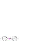
FIG. 3.: Leading order contribution to Eqs. (II). The dot represents the resummation effects in the gluon propagator.

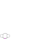
FIG. 4.: Leading order contribution to the electromagnetic mass of charged mesons. The wavy line corresponds to the photon propagator.

REFERENCES

• [1] D. Bailin and A. Love, Phys. Rept. 107, 325 (1984).
• [2] T. Schaefer and E. Shuryak, “Phases of QCD at High Baryon Density,” [nucl-th/0010049].
• [3] K. Rajagopal, “The phases of QCD in heavy ion collisions and compact stars,” [hep-ph/0009058].
• [4] M. Alford, K. Rajagopal, and F. Wilczek, Phys. Lett. B422, 247 (1998).
• [5] J. Gasser and H. Leutwyler, Nucl. Phys. B250, 465 (1985).
• [6] R. Casalbuoni and R. Gatto, Phys. Lett. B464 (1999) 111 [hep-ph/9908227].
• [7] D. T. Son and M. A. Stephanov, Phys. Rev.  D61, 074012 (2000) [hep-ph/9910491]; D. T. Son and M. A. Stephanov, Phys. Rev.  D62, 059902 (2000) [hep-ph/0004095].
• [8] M. Rho, A. Wirzba and I. Zahed, Phys. Lett.  B473, 126 (2000) [hep-ph/9910550].
• [9] D. K. Hong, T. Lee and D. Min, Phys. Lett.  B477, 137 (2000) [hep-ph/9912531].
• [10] C. Manuel and M. H. Tytgat, Phys. Lett.  B479, 190 (2000) [hep-ph/0001095].
• [11] K. Zarembo, Phys. Rev.  D62, 054003 (2000) [hep-ph/0002123].
• [12] S. R. Beane, P. F. Bedaque and M. J. Savage, Phys. Lett.  B483, 131 (2000) [hep-ph/0002209].
• [13] M. Bando, T. Kugo and K. Yamawaki, Phys. Rept.  164, 217 (1988).
• [14] R. D. Pisarski and M. Tytgat, Phys. Rev.  D54, 2989 (1996) [hep-ph/9604404]; M. Kirchbach and D. O. Riska, Nucl. Phys.  A578 (1994) 511.
• [15] S. Weinberg, Phys. Rev. Lett.  18 (1967) 507.
• [16] E. de Rafael, “An introduction to sum rules in QCD,” [hep-ph/9802448].
• [17] D. H. Rischke, Phys. Rev.  D62 (2000) 054017 [nucl-th/0003063].
• [18] G. Ecker, J. Gasser, A. Pich and E. de Rafael, Nucl. Phys.  B321 (1989) 311.
• [19] T. Das, G. S. Guralnik, V. S. Mathur, F. E. Low and J. E. Young, Phys. Rev. Lett.  18 (1967) 759.
• [20] C. Manuel and N. Rius, Phys. Rev.  D59, 054002 (1999) [hep-ph/9806385].
• [21] D. K. Hong, Phys. Rev.  D62 (2000) 091501 [hep-ph/0006105].
• [22] R. Casalbuoni and R. Gatto, Phys. Lett.  B469, 213 (1999) [hep-ph/9909419].
Refer to caption