Abstract

We use an optimized hopping parameter expansion (linear $\delta$-expansion) for the free energy to study the phase transitions at finite temperature and finite charge density in a global U(1) scalar Higgs sector in the continuum and on the lattice at large lattice couplings. We are able to plot out phase diagrams in lattice parameter space and find that the standard second-order phase transition with temperature at zero chemical potential becomes first order as the chemical potential increases.

1 Motivation

In this talk we will tackle phase transitions in the $U(1)$ or $O(2)$ model at finite temperature and chemical potential. The work sketched out here can be found in the papers [1], [2] and builds on that set out in [3] for the case of zero temperature and zero chemical potential.

We are considering the statistical partition function

$$Z=\mbox{\rm Tr}\left(e^{-\beta H-\beta\mu Q}\right)=\mbox{\rm Tr}\left(e^{-\beta H_{\rm eff}}\right)$$

$$Z=\int_{\Phi(0)=\Phi(\beta)}{\cal D}\Phi\exp\left\{-\int_{0}^{\beta}dt_{4}d^{3}\vec{x}{\cal L}_{\rm eff}(\mu)\right\}$$ (1)

where we have now expressed the partition in a Euclidean path integral representation. For a global $U(1)$ scalar field theory the Lagrangian takes the form

$${\cal L}_{\rm eff}=(\nabla_{\mu}\Phi)^{*}(\nabla^{\mu}\Phi)+(m_{0}^{2}-\mu_{0}^{2})\Phi^{*}\Phi+\frac{\lambda_{0}}{4}(\Phi^{*}\Phi)^{2}-\mu_{0}(\Phi^{*}\nabla_{4}\Phi-\Phi\nabla_{4}\Phi^{*})$$ (2)

To tackle phase transitions in this model we need some non-perturbative techniques. The obvious first choice is some type of Monte Carlo technique. Unfortunately in a statistical integration technique $0<e^{-S}<1$ is used as a statistical weight for each possible field configuration but $S_{\rm eff}$ is complex and so cannot be so employed.

We therefore turn to analytic non-perturbative techniques. Both large $N$ approximations and Hartree Fock resumations are hard to extend beyond leading order; instead we shall use a linear delta expansion (LDE) approach. Firstly we will consider an LDE optimization of a $\lambda$ expansion in the continuum and then go on to consider an LDE optimization of a $\kappa$ expansion on the lattice.

2 The Linear Delta expansion

This is an analytic procedure for optimizing a given expansion to give non-perturbative results. The procedure is expressed in the following steps

(1) Use an interpolating action:

$$S\longrightarrow S_{\delta}=S_{0}(\vec{v})+\delta(S-S_{0}(\vec{v}))$$ (3)

(2) Expand in powers of $\delta$ and then truncate at $\delta^{n}$. Setting $\delta=1$ leaves a residual unphysical dependence on $\vec{v}$.

(3) Choose values for $\vec{v}$ order by order in the $\delta$ expansion. The most popular way of choosing the $\vec{v}$ values is by appling the principle of minimal sensitivity (PMS) to some observable.

$$\frac{\partial\left\langle\mathcal{O}\right\rangle_{n}}{\partial v^{i}}=0\Longrightarrow\vec{v}=\vec{v}_{n}$$

$$\left\langle\mathcal{O}\right\rangle_{\rm estimate}=\left\langle\mathcal{O}\right\rangle_{n}(\vec{v}_{n})$$ (4)

One can think of this as a parametized resummation scheme. If $S_{0}$ has the same form as $S$ we have a finite, parametized rescaling of physical parameters, that is, an order by order optimized renormalization scheme choice[4]. The technique yields non-perturbative information from what is, initially, a perturbative (power series) expansion.

3 LDE and $\lambda$ perturbation theory

Following the LDE proceedure, we choose the ${\cal L}_{0}$ Lagrangian to be

$${\cal L}_{0}=(\nabla_{\mu}\Phi)^{*}(\nabla^{\mu}\Phi)+(\Omega^{2}-\mu_{0}^{2})\Phi^{*}\Phi-\mu_{0}(\Phi^{*}\nabla_{4}\Phi-\Phi\nabla_{4}\Phi^{*})$$ (5)

This gives an LDE interpolating lagrangian of the form

$${\cal L}_{\delta}=(\nabla_{\mu}\Phi)^{*}(\nabla^{\mu}\Phi)+(\Omega^{2}-\mu_{0}^{2})\Phi^{*}\Phi-\mu_{0}(\Phi^{*}\nabla_{4}\Phi-\Phi\nabla_{4}\Phi^{*})$$

$$+\delta\left[-(\Omega^{2}-m_{0}^{2})\Phi^{*}\Phi+\frac{\lambda_{0}}{4}(\Phi^{*}\Phi)^{2}\right]$$ (6)

In terms of the partition we have

$$Z=\exp\left\{\delta\left[-(\Omega^{2}-m_{0}^{2})\int dt\frac{\delta^{2}}{\delta j\delta j^{*}}+\frac{\lambda_{0}}{4}\int dt\frac{\delta^{4}}{\delta j^{2}\delta j^{*2}}\right]\right\}Z_{0}[j]$$ (7)

Performing the expansion for the self energy one sees that the expansion is optimized by a ‘mass insertion’ term . The self energy to $O(\delta^{2})$ is

$$\begin{picture}(10.0,5.0)\put(1.0,1.0){\circle*{0.5}} \put(1.0,1.0){\line(1,0){8.0}} \put(5.0,1.0){\circle*{4.0}} \put(9.0,1.0){\circle*{0.5}} \end{picture}=\begin{picture}(10.0,5.0)\put(1.0,1.0){\circle*{0.5}} \put(1.0,1.0){\line(1,0){8.0}} \put(9.0,1.0){\circle*{0.5}} \end{picture}+\begin{picture}(10.0,5.0)\put(1.0,1.0){\circle*{0.5}} \put(1.0,1.0){\line(1,0){8.0}} \put(5.0,2.6){\circle{3.0}} \put(9.0,1.0){\circle*{0.5}} \end{picture}+\begin{picture}(10.0,5.0)\put(1.0,1.0){\circle*{0.5}} \put(1.0,1.0){\line(1,0){8.0}} \put(5.0,1.0){\circle*{1.0}} \put(9.0,1.0){\circle*{0.5}} \end{picture}+\begin{picture}(10.0,5.0)\put(1.0,1.0){\circle*{0.5}} \put(1.0,1.0){\line(1,0){8.0}} \put(5.0,2.6){\circle{3.0}} \put(5.0,5.7){\circle{3.0}} \put(9.0,1.0){\circle*{0.5}} \end{picture}+\begin{picture}(10.0,5.0)\put(1.0,1.0){\circle*{0.5}} \put(1.0,1.0){\line(1,0){8.0}} \put(3.0,2.6){\circle{3.0}} \put(7.0,2.6){\circle{3.0}} \put(9.0,1.0){\circle*{0.5}} \end{picture}+\begin{picture}(10.0,5.0)\put(1.0,1.0){\circle*{0.5}} \put(1.0,1.0){\line(1,0){8.0}} \put(5.0,1.0){\circle{4.0}} \put(9.0,1.0){\circle*{0.5}} \end{picture}+\begin{picture}(10.0,5.0)\put(1.0,1.0){\circle*{0.5}} \put(1.0,1.0){\line(1,0){8.0}} \put(5.0,2.6){\circle{3.0}} \put(5.0,4.0){\circle*{1.0}} \put(9.0,1.0){\circle*{0.5}} \end{picture}+\begin{picture}(10.0,5.0)\put(1.0,1.0){\circle*{0.5}} \put(1.0,1.0){\line(1,0){8.0}} \put(3.0,1.0){\circle*{1.0}} \put(7.0,1.0){\circle*{1.0}} \put(9.0,1.0){\circle*{0.5}} \end{picture}$$ (8)

Renormalization is done using counterterms and this introduces a renormalization scale $M^{2}$. All the resulting integrals are evaluated using a high $T$ expansion. The thermal mass $m_{T}^{2}$ is calculated, and one then fixes the variational parameter using $\frac{\partial m_{T}^{2}}{\partial\eta}=0$, where $\eta^{2}=\Omega^{2}-m_{0}^{2}$.

An typical minimization plot for $m_{T}^{2}$ is seen in Figure 1, along with the resulting phase transition curves in $\{T,\mu\}$ space as compared to the $1$-loop high temperature approximation.

Figure 1: (a) Minimization curve for $m_{T}^{2}$. (b) Phase transition curve in $\{T,\mu\}$ space.

4 LDE and $\kappa$ perturbation theory

The discretized Lagrangian on an asymmetric lattice (different spatial and temporal lattice spacings; $a_{s},a_{t}$) is expressed in terms of dimensionless physical parameters and has the form

$$L_{n}=-\sum_{i}\begin{picture}(10.0,1.0)\put(1.0,1.0){\circle*{0.5}} \put(1.0,1.0){\line(1,0){8.0}} \put(9.0,1.0){\circle*{0.5}} \end{picture}-\begin{picture}(4.0,8.0)\put(2.0,-3.0){\circle*{0.5}} \put(2.0,-3.0){\vector(0,1){8.0}} \put(2.0,5.0){\circle*{0.5}} \end{picture}+(m_{L}^{2}-\mu_{L}^{2})\Phi_{n}^{*}\Phi_{n}+\lambda_{L}(\Phi_{n}^{*}\Phi_{n})^{2}-J_{L}^{*}\Phi_{n}-J_{L}\Phi_{n}^{*}$$ (9)

where $n\equiv(n_{4},\bf{n})$ and the spatial and temporal links are defined by

$$:= \kappa_{s}\left[\Phi_{n_{4},\bf{n}}^{*}\Phi_{n_{4},\bf{n}+\bf{e}_{i}}+\Phi_{n_{4},\bf{n}}\Phi_{n_{4},\bf{n}+\bf{e}_{i}}^{*}\right]$$

$$:= \left[\kappa_{t}\left(1+\mu_{L}\right)\Phi_{n_{4},\bf{n}}^{*}\Phi_{n_{4}+1,\bf{n}}+\kappa_{t}\left(1-\mu_{L}\right)\Phi_{n_{4},\bf{n}}\Phi_{n_{4}+1,\bf{n}}^{*}\right]$$ (10)

The $L_{0}$ Lagrangian is

$$L_{0n}=(\Omega^{2}-\mu_{L}^{2})\Phi_{n}^{*}\Phi_{n}+\lambda_{L}(\Phi_{n}^{*}\Phi_{n})^{2}-j^{*}\Phi_{n}-j\Phi_{n}^{*}$$ (11)

Thus the LDE Lagrangian has the form

$$L_{\delta} =(\Omega^{2}-\mu_{L}^{2})\Phi_{n}^{*}\Phi_{n}+\lambda_{L}(\Phi_{n}^{*}\Phi_{n})^{2}-j^{*}\Phi_{n}-j\Phi_{n}^{*}+\delta\left[-\sum_{i}\begin{picture}(10.0,1.0)\put(1.0,1.0){\circle*{0.5}} \put(1.0,1.0){\line(1,0){8.0}} \put(9.0,1.0){\circle*{0.5}} \end{picture}-\begin{picture}(4.0,8.0)\put(2.0,-3.0){\circle*{0.5}} \put(2.0,-3.0){\vector(0,1){8.0}} \put(2.0,5.0){\circle*{0.5}} \end{picture}\right]$$ (12)

$$+\delta\left[-(\Omega^{2}-m_{L}^{2})\Phi_{n}^{*}\Phi_{n}-(J_{L}^{*}-j^{*})\Phi_{n}-(J_{L}-j)\Phi_{n}^{*}\right]$$

The free energy expansion can be expressed in terms of cumulant averages with respect to the ultra local Lagrangian, $L_{U}$. This is the same as the $L_{\delta}$ Lagrangian but without the spatial and temporal link terms (4). The free energy is

$$F=-\frac{1}{N}\ln Z_{U}-\frac{1}{N}\sum_{j=1}^{\infty}\frac{\delta^{j}}{j!}\left\langle\left(\sum_{n}\begin{picture}(4.0,8.0)\put(2.0,-3.0){\circle*{0.5}} \put(2.0,-3.0){\vector(0,1){8.0}} \put(2.0,5.0){\circle*{0.5}} \end{picture}+\sum_{n,i}\begin{picture}(10.0,1.0)\put(1.0,1.0){\circle*{0.5}} \put(1.0,1.0){\line(1,0){8.0}} \put(9.0,1.0){\circle*{0.5}} \end{picture}\right)^{j}\right\rangle_{C}$$ (13)

and therefore has a diagrammatic representation in terms of connected spatial and temporal links. The variational parameters, $j$ and $\Omega^{2}$, are fixed using the PMS conditions

$$\frac{\partial F}{\partial j}=\frac{\partial F}{\partial\Omega^{2}}=0$$ (14)

and the phase transition is tracked using $\left.\left(\partial F/\partial J_{1}\right)\right|_{J_{1}=0}=-\left\langle\Phi_{1}\right\rangle$. A typical minimization contour plot is seen in Figure 2, along with the resulting phase transition curves in $\{T,\mu_{L}\}$ space. Note that the phase transition becomes first order for sufficently high values of $\mu_{L}$.

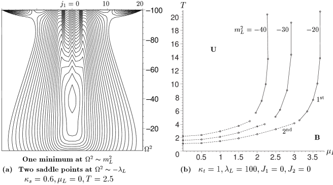
Figure 2: (a) Example minimization contour plot in unbroken regime. (b) Phase transition curves in $\{T,\mu\}$ space. Note that the phase transition becomes first order for large $\mu_{L}$.

5 Conclusions

An LDE optimization of the standard $\lambda$ and hopping parameter expansions has allowed access to some of the truly non-perturbative physics of the global scalar $U(1)$ model at finite $T$ and $\mu_{L}$. On the lattice one finds a first order phase transition at sufficiently large $\mu_{L}$. The approach can be extended to plotting out phase diagrams at finite density for a more complex theory, e.g. gauge theory.

References

- [1] H.F. Jones and P. Parkin, [hep-th/0005069].
- [2] T.S. Evans, H.F. Jones and D. Winder, [hep-th/0008307].
- [3] T.S. Evans, M. Ivin and M. Möbius, Nucl. Phys.B577 (2000) 325.
- [4] P.M. Stevenson, Phys. Rev. D 23 (1981) 2916.