QCD factorization with heavy quarks

Abstract

We further analyze the definition and the calculation of the heavy quark impact factor at next-to-leading (NL) $\log s$ level, and we provide its analytical expression in a previously proposed ${\boldsymbol{k}}$-factorization scheme. Our results indicate that ${\boldsymbol{k}}$-factorization holds at NL level with a properly chosen energy scale, and with the same gluonic Green’s function previously found in the massless probe case.

1 INTRODUCTION

Recent improvements [1] of the next-to-leading $\log x$ (NL$x$) results [2] in the BFKL framework, have stabilized the small-x behaviour in QCD, so that a phenomenological analysis of deep inelastic processes (DIS) seems now possible.

However, both the gluon density (satisfying the improved equation) and the impact factors are needed in order to use ${\boldsymbol{k}}$-factorization [3] to compute DIS or double DIS processes. So far, NL$x$ impact factors have been found for the unphysical case of massless initial quarks and gluons only [3, 4]. Partial features for massive quarks [5, 6] and for colourless sources [7] are known too.

In this talk we present the complete results for the case of initial massive quarks derived in Ref. [8]. These results allowed us to check the validity of the ${\boldsymbol{k}}$-factorization scheme introduced in Ref. [4], or, in other words, to derive probe independent gluon Green’s function with an explicit massive quark impact factor which satisfies the expected collinear properties. Furthermore, we developed as a byproduct some analytical techniques which are needed to deal with two-scale problems, which are hopefully useful to cope with the physical cases also.

2 k-FACTORIZATION IN DIJET PRODUCTION

Following [3], the colour averaged differential cross section for the high-energy scattering of two partons a and b is factorized in a gauge-invariant way into a Green’s function ${\mathcal{G}}_{\omega}$ and impact factors $h_{\mbox{\scriptsize\sf a}}$ and $h_{\mbox{\scriptsize\sf b}}$ (Fig. 1)

$$\frac{{\rm d}\sigma_{\mbox{\scriptsize\sf a}\mbox{\scriptsize\sf b}}}{{\rm d}[{\boldsymbol{k}}_{1}]\,{\rm d}[{\boldsymbol{k}}_{2}]}=\int \frac{{\rm d}\omega}{2\pi i\omega}\,\left(\frac{s}{s_{0}({\boldsymbol{k}}_{1},{\boldsymbol{k}}_{2})}\right)^{\omega}$$ (1)

$$\times h_{\mbox{\scriptsize\sf a}}({\boldsymbol{k}}_{1}){\mathcal{G}}_{\omega}({\boldsymbol{k}}_{1},{\boldsymbol{k}}_{2})h_{\mbox{\scriptsize\sf b}}({\boldsymbol{k}}_{2})~{}.$$

The transverse momenta ${\boldsymbol{k}}_{1}$ and ${\boldsymbol{k}}_{2}$, defined with respect to the incoming momenta $p_{1}$ and $p_{2}$, play the role of hard scales of the process.

At the next-to-leading $\log x$ (NL$x$) accuracy the Green’s function ${\mathcal{G}}_{\omega}$ has the following general form

$${\mathcal{G}}_{\omega}=(1+\overline{\alpha}_{s}H_{L}) \left[1-\frac{\overline{\alpha}_{s}}{\omega}(K_{0}+K_{NL})\right]^{-1}\!$$

$$\times(1+\overline{\alpha}_{s}H_{R})~{},$$ (2)

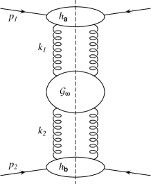
Figure 1: Diagrammatic representation of ${\boldsymbol{k}}$-factorization.

where $K_{0}$ and $K_{NL}$ are the leading $\log x$ (L$x$) and the NL$x$ BFKL kernels [2] respectively, $H_{R}(H_{L})$ are operator factors introduced in [4] so as to provide partonic impact factors free of double $\log$ collinear divergences and $\overline{\alpha}_{s}=\alpha_{s}N_{c}/\pi$ is the dimensionless strong coupling constant.

As explained in [4], the identification of the second order impact factors, $h_{\mbox{\scriptsize\sf a}}^{(1)}$ and $h_{\mbox{\scriptsize\sf b}}^{(1)}$, is affected by a double factorization scheme ambiguity, due to both the choice of the scale $s_{0}$ and of the kernels $H_{R}(H_{L})$.

3 FACTORIZATION SCHEME AND CALCULATIONAL PROCEDURE

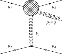
Figure 2: Real gluon emission in the fragmentation region of quark ${\sf a}$.

Let’s consider first the high-energy scattering of two partons ${\sf a}$ and ${\sf b}$ where ${\sf a}={\sf q}$ is a heavy quark of mass $m$ with real emission of an extra gluon ${\sf g}$ that we assume in the heavy quark fragmentation region (Fig. 2). In terms of invariants $s_{2}=(q+p_{4})^{2}\gg s_{1}=(p_{3}+q)^{2}$. The Born differential cross section in this high energy region was calculated in [8]. Though complicated at first sight it reduces, as expected to the known [4] result for $m\rightarrow 0$, and matches the L$x$ differential cross section

$$\frac{{\rm d}\sigma^{(L)}_{\mbox{\scriptsize\sf q}\mbox{\scriptsize\sf g}\mbox{\scriptsize\sf b}}}{{\rm d}z_{1}\,{\rm d}[{\boldsymbol{k}}_{1}]\,{\rm d}[{\boldsymbol{k}}_{2}]} =h_{\mbox{\scriptsize\sf q}}^{(0)}({\boldsymbol{k}}_{1})\,h_{\mbox{\scriptsize\sf b}}^{(0)}({\boldsymbol{k}}_{2})$$

$$\times\frac{\overline{\alpha}_{s}}{{\boldsymbol{q}}^{2}\Gamma(1-\varepsilon)\mu^{2\varepsilon}}\,\frac{1}{z_{1}}~{},$$ (3)

in the limit $z_{1}\rightarrow 0$, being $z_{1}$ the momentum fraction of $k_{1}=p_{1}-p_{3}$ with respect to the incoming momentum $p_{1}$, $h^{(0)}({{\boldsymbol{k}}_{i}})$ the leading order impact factor and ${\boldsymbol{q}}={\boldsymbol{k}}_{1}+{\boldsymbol{k}}_{2}$.

However, as pointed out in [8], for eq.(3) to be a good approximation to the total result, we should require ($q=|{\boldsymbol{q}}|,k_{i}=|{\boldsymbol{k}}_{i}|$)

$$z_{1}\ll q/k_{1}~{},\quad q/m~{},\quad k_{1}/m~{}.$$ (4)

The first two cutoffs can be summarized by $z_{1}<q/Max(k_{1},m)$, which is a coherence condition for the case of heavy quarks, saying that the rapidity of the gluon cannot exceed that of the final quark.

By integrating the leading expression (3) with the constraints (4) in the fragmentation region $z_{1}>q/\sqrt{s}$, an estimate of the leading contribution contained in the complete result, which should be subtracted out in order to yield the impact factor in the massive quark case, was found [8]. Then, by considering both real and virtual contributions to the fragmentation function $F_{\mbox{\scriptsize\sf q}}(z_{1},{\boldsymbol{k}}_{1},{\boldsymbol{k}}_{2})$, we introduced the following definition of the impact factor $h_{\mbox{\scriptsize\sf q}}^{(1)}({\boldsymbol{k}})$:

$$\int_{q/\sqrt{s}}^{1}{\rm d}z_{1}\int{\rm d}[{\boldsymbol{k}}_{1}]F_{\mbox{\scriptsize\sf q}}(z_{1},{\boldsymbol{k}}_{1},{\boldsymbol{k}}_{2})=$$

$$=h_{\mbox{\scriptsize\sf q}}^{(1)}({\boldsymbol{k}}_{2})+\int{\rm d}[{\boldsymbol{k}}_{1}]\,\overline{\alpha}_{s}\,h_{\mbox{\scriptsize\sf q}}^{(0)}({\boldsymbol{k}}_{1})\,K_{0}({\boldsymbol{k}}_{1},{\boldsymbol{k}}_{2})\,$$

$$\qquad\times\left(\log\frac{\sqrt{s}}{Max(k_{1},m)}-\log\frac{q}{k_{1}}\Theta_{qk_{1}}\right)~{}.$$ (5)

Compared to the subtraction (or factorization) scheme adopted in [4] for $m=0$, the expression (5) differs by the replacement $k_{1}\rightarrow Max(k_{1},m)$, which leads, by adding the symmetrical fragmentation region, to the choice for the factorized scale in eq.(1)

$$s_{0}=Max(k_{1},m_{1})Max(k_{2},m_{2})~{},$$ (6)

$m_{1}$ being the mass of quark ${\sf a}$ and $m_{2}$ the mass of quark ${\sf b}$, and in particular contains the subtraction term $\log q/k_{1}\Theta_{qk_{1}}$ which provides the expression ($H_{R}=H_{L}^{\dagger}=H$)

$$H({\boldsymbol{k}}_{1},{\boldsymbol{k}}_{2})=-\frac{1}{{\boldsymbol{q}}^{2}\Gamma(1-\varepsilon)\mu^{2\varepsilon}}\,\log\frac{q}{k_{1}}\;\Theta_{qk_{1}}~{},$$ (7)

for the $H$ kernel in the ${\boldsymbol{k}}$-factorization formula.

In order to simplify the subsequent calculations, the known result [4] for $m=0$ was used and only the difference for a non vanishing mass

$$\Delta F_{\mbox{\scriptsize\sf q}} (z_{1},{\boldsymbol{k}}_{1},{\boldsymbol{k}}_{2})=$$

$$=F_{\mbox{\scriptsize\sf q}}(z_{1},{\boldsymbol{k}}_{1},{\boldsymbol{k}}_{2})-F^{m=0}_{\mbox{\scriptsize\sf q}}(z_{1},{\boldsymbol{k}}_{1},{\boldsymbol{k}}_{2})~{},$$ (8)

was explicitly computed. Then, we found the following relationship between the massless quark and the heavy quark impact factors

$$h_{\mbox{\scriptsize\sf q}}^{(1)} ({\boldsymbol{k}}_{2})=h_{\mbox{\scriptsize\sf q},m=0}^{(1)}({\boldsymbol{k}}_{2})+$$ (9)

$$+\int_{0}^{1}{\rm d}z_{1}\int{\rm d}[{\boldsymbol{k}}_{1}]\Delta F_{\mbox{\scriptsize\sf q}}(z_{1},{\boldsymbol{k}}_{1},{\boldsymbol{k}}_{2})$$

$$+\int{\rm d}[{\boldsymbol{k}}_{1}]\,\overline{\alpha}_{s}\,h_{\mbox{\scriptsize\sf q}}^{(0)}({\boldsymbol{k}}_{1})\,K_{0}({\boldsymbol{k}}_{1},{\boldsymbol{k}}_{2})\,\log\frac{m}{k_{1}}\,\Theta_{m\,k_{1}}~{}.$$

Notice that the integration limits in $z_{1}$ have been extended down to $z_{1}=0$. Since $\Delta F_{\mbox{\scriptsize\sf q}}$ is regular at $z_{1}=0$ this change introduces only a negligible error of order $1/s$.

4 MELLIN TRANSFORM AND ITS INVERSE

In order to perform the calculation outlined in eq.(9), we proceeded in two steps. First, the ${\boldsymbol{k}}_{1}$ integration was performed analytically by reducing the ${\boldsymbol{k}}_{1}$-integrals to two denominators. Then, the virtual contribution [9] was considered and organized in terms of momentum fraction integrals only. Finally, summing up real and virtual contributions to the fragmentation vertex we obtained an expression for the difference $\Delta F_{\mbox{\scriptsize\sf q}}({\boldsymbol{k}}_{2})$, arising from the second term in the r.h.s. of eq.(9). To perform the last integrations we calculated its Mellin transform

$$\Delta\tilde{F}_{\mbox{\scriptsize\sf q}}(\gamma) =\Gamma(1+\varepsilon)\,(m^{2})^{-\varepsilon}$$

$$\times\int{\rm d}[{\boldsymbol{k}}_{2}]\left(\frac{{\boldsymbol{k}}_{2}^{2}}{m^{2}}\right)^{\gamma-1}\Delta F_{\mbox{\scriptsize\sf q}}({\boldsymbol{k}}_{2})~{},$$

which allowed us to disentangle the $(m/k)$-dependence, yielding

$$\Delta \tilde{F}_{\mbox{\scriptsize\sf q}}(\gamma)=A_{\varepsilon}\,(m^{2})^{\varepsilon}$$

$$\times\frac{\Gamma(\gamma+\varepsilon)\Gamma(1-\gamma-2\varepsilon)\Gamma^{2}(1-\gamma-\varepsilon)}{8\Gamma(2-2\gamma-2\varepsilon)}$$

$$\times\bigg{[}\frac{1+\varepsilon}{\gamma+2\varepsilon}+\frac{2}{1-2\gamma-4\varepsilon}$$

$$\qquad\times\left(\frac{1}{1-\gamma-2\varepsilon}-\frac{1}{3-2\gamma-2\varepsilon}\right)\bigg{]}~{},$$ (10)

where $A_{\varepsilon}$ is a constant that contains the dependence on the strong coupling constant and some colour factors.

It is straightforward, though not trivial, to show that eq.(10) converges only in the small band $1-2\varepsilon<Re\gamma<1-\varepsilon$. The inverse Mellin transform was thus defined as

$$\Delta F_{\mbox{\scriptsize\sf q}}({\boldsymbol{k}}_{2})=\frac{1}{m^{2}} \int_{1-2\varepsilon<Re\gamma<1-\varepsilon}\frac{{\rm d}\gamma}{2\pi i}$$

$$\times\left(\frac{{\boldsymbol{k}}_{2}^{2}}{m^{2}}\right)^{-\gamma-\varepsilon}\Delta\tilde{F}_{\mbox{\scriptsize\sf q}}(\gamma)~{}.$$

Then, displacing the integration contour around the positive or the negative real semiaxis, i.e. enclosing all the poles placed either at $\gamma\geq 1-\varepsilon$ or $\gamma\leq 1-2\varepsilon$, we calculated the different corrections of order $\mathcal{O}(m/k_{2})^{n}$ or $\mathcal{O}(k_{2}/m)^{n}$ to the impact factor in the limits ${\boldsymbol{k}}_{2}^{2}>m^{2}$ and ${\boldsymbol{k}}_{2}^{2}<m^{2}$ respectively.

5 IMPACT FACTOR

Our final result for the heavy quark impact factor at the next-to-leading level reads

$$h_{\mbox{\scriptsize\sf q}}({\boldsymbol{k}}_{2})=h_{\mbox{\scriptsize\sf q}}^{(1)}({\boldsymbol{k}}_{2})\big{|}_{sing}+h_{\mbox{\scriptsize\sf q}}({\boldsymbol{k}}_{2})\big{|}_{finite}~{},$$ (11)

where the singular piece is defined as

$$h_{\mbox{\scriptsize\sf q}}^{(1)} ({\boldsymbol{k}}_{2})\big{|}_{sing}=\delta h_{1}^{(1)}({\boldsymbol{k}}_{2})$$ (12)

$$+h_{\mbox{\scriptsize\sf q}}^{(0)}({\boldsymbol{k}}_{2})\,\frac{\alpha_{s}N_{c}}{2\pi}\left(-\frac{3}{2}\log\frac{{\boldsymbol{k}}_{2}^{2}}{m^{2}}\right)\Theta_{k_{2}\,m}~{},$$

and

$$h_{\mbox{\scriptsize\sf q}} ({\boldsymbol{k}}_{2})\big{|}_{finite}=h_{\mbox{\scriptsize\sf q}}^{(0)}(\alpha_{s}({\boldsymbol{k}}_{2}))\bigg{\{}1+\frac{\alpha_{s}N_{c}}{2\pi}$$

$$\times \bigg{[}{\mathcal{K}}-\frac{\pi^{2}}{6}-\bigg{(}\frac{3}{2}+\sum_{Re\gamma>1}Res[\tilde{h}(\gamma)]\bigg{)}\Theta_{k_{2}\,m}$$

$$+\bigg{(}2+\sum_{Re\gamma<1}Res[\tilde{h}(\gamma)]\bigg{)}\Theta_{m\,k_{2}}\bigg{]}\bigg{\}}~{},$$ (13)

is the finite contribution, with

$${\mathcal{K}}=\frac{67}{18}-\frac{\pi^{2}}{6}-\frac{5n_{f}}{9N_{c}}~{}.$$ (14)

As for the massless case, the singularities proportional to $(11/6-n_{f}/3N_{c})$, the beta function, were absorbed by the running strong coupling constant $\alpha_{s}({\boldsymbol{k}}_{2})$. The function $\tilde{h}(\gamma)$ provides the corrections [8] of order $\mathcal{O}(m/k_{2})$ and $\mathcal{O}(k_{2}/m)$ to the impact factor for ${\boldsymbol{k}}_{2}^{2}>m^{2}$ and ${\boldsymbol{k}}_{2}^{2}<m^{2}$ respectively.

Notice that all double $\log$ contributions of type $1/\varepsilon^{2}$ and $1/\varepsilon\log({\boldsymbol{k}}_{2}^{2}/m^{2})$ appearing in the intermediate steeps of the calculation canceled out which means that indeed our subtraction of the leading kernel was effective, thus lending credit to the scale (6) and to the $H$-kernel (7). The remaining singularities of the impact factor are single logarithmic ones $\sim~{}1/\varepsilon$. In fact, the impact factor is actually finite, with the expected $\log({\boldsymbol{k}}_{2}^{2}/m^{2})$ dependence predicted by the DGLAP equations, the divergent piece $\delta h_{1}^{(1)}({\boldsymbol{k}}_{2})$ in eq.(12), see [8], can be interpreted as a finite mass scale change, i.e. the scale leading to a finite massive quark impact factor differs from eq.(6) by a finite renormalization of the quark mass, which is a normal ambiguity in this type of problems.

6 CONCLUSIONS

Starting from the explicit squared matrix element for gluon emission we motivated the subtraction of the leading term, and we performed the ${\boldsymbol{k}}_{1}$ and $z_{1}$ integrals needed to provide an explicit result for the heavy quark impact factor.

Even if the cross section being investigated is unphysical, the relevance of our results stems from the consistency of the following features: (i) the validity of the ${\boldsymbol{k}}$-factorization formula (1) with scale $s_{0}=Max(k_{1},m_{1})Max(k_{2},m_{2})$; (ii) the explicit expression of the impact factor with factorizable single logarithmic collinear divergences, and (iii) the probe-independence of the subleading $H$-kernels of the CC scheme [4], defined in eq.(7).

Of course, the real problem is to provide an explicit expression for the DIS impact factors. But – if the lesson learned form the L and NL kernels is still valid – the impact factor’s magnitude is not expected to be much different from their approximate collinear evaluation.

References

• [1] G.P. Salam, JHEP 9807(1998)019 [hep-ph/9806482]; M. Ciafaloni and D. Colferai, Phys. Lett. B 452 (1999) 372 [hep-ph/9812366]; M. Ciafaloni, D. Colferai and G.P. Salam, Phys. Rev. D 60 (1999) 114036 [hep-ph/9905566].
• [2] V.S. Fadin and L.N. Lipatov, Phys. Lett. B 429 (1998) 127 [hep-ph/9802290]; M. Ciafaloni and G. Camici, Phys. Lett. B 430 (1998) 249 [hep-ph/9803389].
• [3] M. Ciafaloni, Phys. Lett. B 429 (1998) 363 [hep-ph/9801322].
• [4] M. Ciafaloni and D. Colferai, Nucl. Phys. B 538 (1999) 187 [hep-ph/9806350].
• [5] V.S. Fadin, these Proceedings.
• [6] V.S. Fadin, R. Fiore, M.I. Kotsky and A. Papa, Phys. Rev. D 61 (2000) 094006 [hep-ph/9908265].
• [7] V.S. Fadin and A.D. Martin, Phys. Rev. D 60 (1999) 114008 [hep-ph/9904505].
• [8] M. Ciafaloni and G. Rodrigo, JHEP 0005(2000)042 [hep-ph/0004033].
• [9] V.S. Fadin and L.N. Lipatov, Nucl. Phys. B 406 (1993) 259; V.S. Fadin, R. Fiore and A. Quartarolo, Phys. Rev. D 50 (1994) 2265; Phys Rev. D 50 (1994) 5893; V.S. Fadin, R. Fiore and M.I. Kotsky, Phys. Lett. B 359 (1995) 181; B 387 (1996) 593; B 389 (1996) 737.
• [10] M. Taiuti, University of Florence Thesis (February 2000), unpublished.