Chiral Expansion Theory at Vector Meson Scale

Abstract

We study physics on $\rho(770)$ and $\omega(782)$ in framework of chiral constituent quark model. The effective action is derived by proper vertex method, which can capture all order information of chiral expansion. The $N_{c}^{-1}$ expansion is also studied systematically. It is shown that the momentum expansion at vector meson energy scale converges slowly, and the loop effects of pseudoscalar meson play an important role at this energy scale. We provide a method to prove the unitarity of S-matrix in any low-energy effective theory of QCD. Phenomenologically, we study decays for $\rho\rightarrow\pi\pi$, $\rho\rightarrow e^{+}e^{-}$, $\omega\rightarrow\pi^{+}\pi^{-}$, $\rho^{\pm}\rightarrow\gamma\pi^{\pm}$ and $\omega\rightarrow\gamma\pi^{0}$, $\rho^{0}-\omega$ mixing and their mass splitting, pion form factor, $I=l=1$ phase shift and light quark masses at vector meson energy scale. These results include all order contribution of vector meson momentum expansion and is up to next to leading order of $N_{c}^{-1}$ expansion. All of these theoretical predictions agree with data very well. The unitarity of S-matrix yielded by this framework is examined. The Breit-Winger formula for resonance propagator is derived.

12.39.-x,11.30.Rd,12.40.Yx,12.40.Vv,13.25.-k,13.75.Lb

I Introduction

In past thirty years, the effective theory studies on physics of light vector meson resonances($\rho$, $\omega$, $K^{*}$ and $\phi$) have attracted much interests. Works in this field have helped us to understand various aspects on low energy QCD and properties of light vector mesons. A challenging subject in these studies is to construct a well-defined chiral expansion theory at vector meson scale. In ref.[1] authors have developed a chiral expansion theory including vector mesons. In this framework one can successfully deal with two-vector-meson processes (one vector meson is in initial state and one is in final state)[2]. However, it was also pointed out in ref.[1] that this framework is failed to study single-vector-meson processes. So far, the most studies on single-vector-meson processes are still limited at the lowest order of vector meson four-momentum expansion and $N_{c}^{-1}$ expansion. Theoretical reason is that convergence of momentum expansion in these processes is unclear, and technical reason is that the calculation beyond the leading order is very difficult. For example, method of chiral perturbative theory(ChPT)[4] is impractical for these processes because more and more free parameters are required as perturbative order raising. Obviously, this is a serious problem that has to be resolved, since it makes the models’ calculations being not controlled approximations in that error bars can not be put on the predictions. Although there are some attempts to resolve these problem in terms of resumming the momentum expansion at vector meson scale[3], the resummation was not yet used in phenomenological studies of vector mesons so far. The purposes of this present paper are to study chiral expansion in single-vector-meson processes systematically in the framework of chiral quark model, and to overcome the difficulties mentioned in above. Our studies will be not only resumming momentum expansion of vector mesons, but also beyond the leading order of $N_{c}^{-1}$ expansion.

The convergence of the chiral expansion is a fundamental requirement for any chiral model. In this paper, a broad class of chiral quark model will be checked by this requirement. The simplest version of the chiral quark model is in ref.[5], that was originated by Weinberg[6], and has been extended to some different versions[7, 8, 9, 10]. The constituent quark model in ref.[5] is different from other versions in refs.[7, 8, 9, 10]. The massless pseudoscalar mesons are treated as fundamental dynamical field degrees of freedom in the former, but are treated as composite fields of quarks in the latter. In section 5 of this paper, we will show that the chiral quark models in refs.[7, 8, 9, 10] can not yield convergent chiral expansion in single-vector-meson processes, and the effective lagrangian derived from these chiral quark models can not give unitarity S-matrix for vector meson physics. Therefore, in this paper, our studies will be within the framework of a chiral constituent quarks model proposed by Manohar and Georgi[5](quote as MG model hereafter). It is the simplest and practical model for achieving our goal. In view of this model, in energy region between chiral symmetry spontaneously breaking(CSSB) scale($\Lambda_{\chi}\simeq 2\pi f_{\pi}\simeq 1.16$GeV) and the confinement scale($\Lambda_{QCD}\sim 0.1-0.3$GeV), the dynamical field degrees of freedom are constituent quarks(quasi-particle of quarks), gluons and Goldstone bosons associated with CSSB(it is well-known that these Goldstone bosons correspond to lowest pseudoscalar octet). In this quasiparticle description, the effective coupling between gluon and quarks is small and the important interaction is the coupling between quarks and Goldstone bosons. The effective action describing interaction of Goldstone bosons can be obtained via integrating out freedoms of quark fields.

The MG model and its extension have been studied continually during the last fifteen years and got great success in different aspects of phenomenological predictions in hadron physics[11]. Low energy limit of the model has been examined successfully[7, 12]. In this present paper, the MG model will be extended to include lowest vector meson resonances(quote as extended Manohar-Georgi model or EMG model hereafter) in terms of WCCWZ realization for spin-1 mesons[13, 14]. The advantages of approach of the MG model are that, in principle, high order contribution of the chiral expansion can be computed completely, and only fewer free parameters are required. So far, however, there are still no any systematic studies beyond the lowest order of the chiral expansion due to technical difficulties. After freedoms of fermions are integrated out, traditionally, the determinant of Dirac operator are regularized by some standard methods, such as Schwinger proper time method[15], or heat kernel method[16], and are expanded in powers of momentum of mesons. In terms of this method, the effective action can keep chiral symmetry explicitly order by order. However, it is very difficult to capture arbitrary order contribution in chiral expansion by means of the above method. In this present paper, we will propose another equivalent method to evaluate the effective action via calculating one-loop diagrams of constituent quarks directly. We call it as proper vertex expansion method. By this method, the effective action is expanded in numbers of external vertices instead of external momentum. The effective action with n external vertices is just connective n-point Green function of EMG model in presence of external fields. It includes all order contribution of the momentum expansion. Thus in terms of this method, the chiral theory at vector meson energy scale can be studies up to all orders of the momentum expansion.

Another challenging subject is to study vector meson physics beyond large $N_{c}$ limit. In the other words, how can we calculate meson loops systematically and consistently? At vector meson energy scale, it can be expected that the contributions from pseudoscalar meson loops play important and highly nontrivial role. This is due to the following reasons: 1)Empirically, for vector meson physics, the contribution from pseudoscalar meson loops is about $\Gamma_{\rho}:m_{\rho}\simeq 20\%$. The conclusion is obtained because the width of $\rho$-meson is generated dynamically by pion loops and $\Gamma_{\rho}:m_{\rho}$ is suppressed by $N_{c}^{-1}$ expansion according to standard $N_{c}^{-1}$ argument[17]. It indicates that the contribution from pseudoscalar meson loops is not small so that it can not be omitted simply. 2) Since both pseudoscalar mesons and constituent quarks are fundamental dynamical field degrees of freedoms at this energy scale, theoretically, loop effects of pseudoscalar mesons should be also considered as well when effective action is derived by loop effects of constituent quarks. 3)For physical value $N_{c}=3$, the $N_{c}^{-1}$ expansion is not convergent very rapidly. Due to the above reasons, in this paper we will also study contribution from pseudoscalar meson loops systematically. The calculations on meson loops will suffer ultraviolet(UV) divergent difficulty. At vector meson energy scale, loop effects of pseudoscalar mesons cause $\phi-\omega$ mixing which will destroy OZI rule[18] if this contribution is not to be an appropriate value. In the other words, it can insure OZI rule for $\phi$ to choose an UV cut-off appropriately. Thus, very fortunately, the OZI rule for $\phi$ provides a natural way to determine all UV-dependent contributions in the meson loop calculations.

The unitarity of S-matrix is a fundamental requirement for any quantum field theory. It is well-known that the unitarity of S-matrix of an effective theory can not be insured in full energy region, but only be insured in energy region below an energy cut-off. The consistency of this effective theory requires masses of all resonances should be smaller than this cut-off. In the other words, it indicates that the cut-off $\Lambda_{\rm EMG}$ in EMG model should satisify $\Lambda_{\rm EMG}>m_{\omega}$ for SU(2) and $\Lambda_{\rm EMG}>m_{\phi}$ for SU(3) at least. In general, a low energy effective field theory of QCD is a well-defined perturbative theory in $N_{c}^{-1}$ expansion. Thus the unitarity of S-matrix of low energy effective field theory has to be satisfied in order by order in $N_{c}^{-1}$ expansion. For EMG model, the unitarity of S-matrix will be examined explicitly in this paper. We will see that the meson-loop effects play an essential role for meeting the requirement of the unitarity.

The phenomenology of vector meson physics is very rich. For example, the vector meson dominance(VMD) and universal coupling for vector mesons, which are good approximation for vector meson physics[19], should be satisfied in the leading order of the chiral expansion. In this present paper, we will achieve various phenomenological results: 1)The decays for $\rho\rightarrow\pi\pi$, $\rho\rightarrow e^{+}e^{-}$. 2) Dynamical width for $\rho$-meson and Breit-Wigner formula for propagator of resonance. 3) $\rho^{0}-\omega$ mixing and $\omega\rightarrow\pi^{+}\pi^{-}$ decay. The mass difference between $\rho$ and $\omega$ are also predicted. We will show that, for resonance particles with large width(e.g., $\rho$), the mass parameter in its propagator is not just the its physics mass. 4)Pion form factor and $I=1,\;l=1$ pion-pion phase shift. Some nontrivial phase in pion form factor are revealed too. 5) Individual light current quark masses at vector meson energy scale. The quark masses are model-dependent and are necessary to extend our study to $K^{*}$ and $\phi$ mesons. 6)The anomalous decays $\rho^{\pm}\rightarrow\gamma\pi^{\pm}$ and $\omega\rightarrow\gamma\pi$. All above results resum all information of the momentum expansion of vector mesons and are up to the next to leading order of $N_{c}^{-1}$ expansion.

The paper is organized as follows. In sect. 2 the Manohar-Georgi model and its extension are reviewed. In sect. 3, the relevant effective action is derived at the leading order of $N_{c}^{-1}$ expansion. This effective action includes all order contribution of the chiral expansion in powers of vector meson four-momentum square. The calculation on pseudoscalar meson loops will be included in the following sections. In sect. 4, decays for $\rho\rightarrow\pi\pi$ and $\rho^{0}\rightarrow e^{+}e^{-}$ are studied. In sect. 5, the unitarity of S-matrix is examined explicitly and Breit-Wigner formula for $\rho$-propagator is obtained. In sect. 6, the $\rho^{0}-\omega$ mixing and $\omega\rightarrow\pi\pi$ decay are studied. The isospin breaking parameter $m_{d}-m_{u}$ is predicted at energy scale $\mu=m_{\rho}$. In sect. 7, the anomalous decays for $\rho^{\pm}\rightarrow\gamma\pi^{\pm}$ and $\omega\rightarrow\gamma\pi$ are predicted. In sect. 8, pion form factor, $I=1,\;l=1$ $\pi-\pi$ phase shift and $\rho^{0}-\omega$ mass difference are studied. The light quark masses are predicted in sect. 9 and a brief summary is in sect. 10.

II Manohar-Georgi model and its extension

For interpreting physics below CSSB scale, Manohar and Georgi provides a QCD-inspired description on the simple constituent quark model. At chiral limit, it is parameterized by the following $SU(3)_{{}_{V}}$ invariant chiral constituent quark lagrangian

$${\cal L}_{\chi} = i\bar{\psi}(/\!\!\!\partial+/\!\!\!\Gamma+g_{{}_{A}}{/\!\!\!\!\Delta}\gamma_{5})\psi-m\bar{\psi}\psi+\frac{F^{2}}{16}Tr_{f}\{\nabla_{\mu}U\nabla^{\mu}U^{{\dagger}}\}.$$ (2.1)

Here $Tr_{f}$ denotes trace in SU(3) flavour space, $\bar{\psi}=(\bar{u},\bar{d},\bar{s})$ are constituent quark fields, $g_{{}_{A}}=0.75$ can be fitted by beta decay of neutron. The $\Delta_{\mu}$ and $\Gamma_{\mu}$ are defined as follows,

$$\Delta_{\mu} = \frac{1}{2}\{\xi^{{\dagger}}(\partial_{\mu}-ir_{\mu})\xi-\xi(\partial_{\mu}-il_{\mu})\xi^{{\dagger}}\},$$ (2.2)

$$\Gamma_{\mu} = \frac{1}{2}\{\xi^{{\dagger}}(\partial_{\mu}-ir_{\mu})\xi+\xi(\partial_{\mu}-il_{\mu})\xi^{{\dagger}}\},$$ (2.3)

and covariant derivative are defined as follows

$$\nabla_{\mu}U = \partial_{\mu}U-ir_{\mu}U+iUl_{\mu}=2\xi\Delta_{\mu}\xi,$$ (2.4)

$$\nabla_{\mu}U^{{\dagger}} = \partial_{\mu}U^{{\dagger}}-il_{\mu}U^{{\dagger}}+iU^{{\dagger}}r_{\mu}=-2\xi^{{\dagger}}\Delta\xi^{{\dagger}},$$ (2.5)

where $l_{\mu}=v_{\mu}+a_{\mu}$ and $r_{\mu}=v_{\mu}-a_{\mu}$ are linear combinations of external vector field $v_{\mu}$ and axial-vector field $a_{\mu}$, $\xi$ associates with non-linear realization of spontaneously broken global chiral symmetry $G=SU(3)_{L}\times SU(3)_{R}$ introduced by Weinberg[13],

$$\xi(\Phi)\rightarrow g_{R}\xi(\Phi)h^{{\dagger}}(\Phi)=h(\Phi)\xi(\Phi)g_{L}^{{\dagger}},\hskip 36.135ptg_{L},g_{R}\in G,\;\;h(\Phi)\in H=SU(3)_{{}_{V}}.$$ (2.6)

Explicit form of $\xi(\Phi)$ is usual taken

$$\xi(\Phi)=\exp{\{i\lambda^{a}\Phi^{a}(x)/2\}},\hskip 72.26999ptU(\Phi)=\xi^{2}(\Phi),$$ (2.7)

where the Goldstone boson $\Phi^{a}$ are treated as pseudoscalar meson octet. The constituent quark fields transform as matter fields of SU(3)${}_{{}_{V}}$,

$$\psi\longrightarrow h(\Phi)\psi,\hskip 72.26999pt\bar{\psi}\longrightarrow\bar{\psi}h^{{\dagger}}(\Phi).$$ (2.8)

$\Delta_{\mu}$ is SU(3)${}_{{}_{V}}$ invariant field gradients and $\Gamma_{\mu}$ transforms as field connection of SU(3)${}_{{}_{V}}$

$$\Delta_{\mu}\longrightarrow h(\Phi)\Delta_{\mu}h^{{\dagger}}(\Phi),\hskip 57.81621pt\Gamma_{\mu}\longrightarrow h(\Phi)\Gamma_{\mu}h^{{\dagger}}(\Phi)+h(\Phi)\partial_{\mu}h^{{\dagger}}(\Phi).$$ (2.9)

Thus the lagrangian( 2.1) is invariant under $G_{\rm global}\times G_{\rm local}$.

For achieving the purposes of this present paper, MG model must be extended to including lowest vector meson resonance and beyond chiral limit. The light quark mass matrix ${\cal M}={\rm diag}\{m_{u},m_{d},m_{s}\}$ is usually included into external spin-0 fields, i.e., $\tilde{\chi}=s+ip$, where $s=s_{\rm ext}+{\cal M}$, $s_{\rm ext}$ and $p$ are scalar and pseudoscalar external fields respectively. The chiral transformation for $\tilde{\chi}$ is

$$\tilde{\chi}\rightarrow g_{{}_{R}}\tilde{\chi}g_{{}_{L}}^{{\dagger}}.$$ (2.10)

Thus $\tilde{\chi}$ and $\tilde{\chi}^{{\dagger}}$ together with $\xi$ and $\xi^{{\dagger}}$ can form SU(3)_V invariant scalar source $\xi^{{\dagger}}\tilde{\chi}\xi^{{\dagger}}+\xi\tilde{\chi}^{{\dagger}}\xi$ pseudoscalar source $(\xi^{{\dagger}}\tilde{\chi}\xi^{{\dagger}}-\xi\tilde{\chi}^{{\dagger}}\xi)\gamma_{5}$. Then current quark mass dependent term is written

$$-\frac{1}{2}\bar{q}(\xi^{{\dagger}}\tilde{\chi}\xi^{{\dagger}}+\xi\tilde{\chi}^{{\dagger}}\xi)q-\frac{\kappa}{2}\bar{q}(\xi^{{\dagger}}\tilde{\chi}\xi^{{\dagger}}-\xi\tilde{\chi}^{{\dagger}}\xi)\gamma_{5}q.$$ (2.11)

Eq. (2.11) will return to standard quark mass term of QCD lagrangian, $\bar{\psi}{\cal M}\psi$, in absence of pseudoscalar mesons at high energy for arbitrary $\kappa$. It means that the symmetry and some underlying constrains of QCD can not fixed the coupling between pseudoscalar mesons and constituent quarks. Hence $\kappa$ is treated as an initial parameter of the model and will be fitted phenomenologically.

From the viewpoint of chiral symmetry only, an alternative scheme for incorporating vector mesons was suggested by Weinberg[13] and developed by Callan, Coleman et. al[14]. In this treatment, vector meson resonances $V_{\mu}$ transform homogeneously under SU(3)_V,

$$V_{\mu}\rightarrow h(\Phi)V_{\mu}h^{{\dagger}}(\Phi),$$ (2.12)

where

$$V_{\mu}(x)={\bf\lambda\cdot V}_{\mu}=\sqrt{2}\left(\begin{array}[]{ccc}\frac{\rho^{0}_{\mu}}{\sqrt{2}}+\frac{\omega_{\mu}}{\sqrt{2}}&\rho^{+}_{\mu}&K^{*+}_{\mu}\\ \rho^{-}_{\mu}&-\frac{\rho^{0}_{\mu}}{\sqrt{2}}+\frac{\omega_{\mu}}{\sqrt{2}}&K^{*0}_{\mu}\\ K^{*-}_{\mu}&\bar{K}^{*0}_{\mu}&\phi_{\mu}\end{array}\right).$$ (2.13)

Then extended Manohar-Georgi model(EMG model) is parametered by the following SU(3)${}_{{}_{V}}$ invariant lagrangian

$${\cal L}_{\chi} = i\bar{q}(/\!\!\!\partial+/\!\!\!\Gamma+g_{{}_{A}}{/\!\!\!\!\Delta}\gamma_{5}-i/\!\!\!V)q-m\bar{q}q-\frac{1}{2}\bar{q}(\xi^{{\dagger}}\tilde{\chi}\xi^{{\dagger}}+\xi\tilde{\chi}^{{\dagger}}\xi)q-\frac{\kappa}{2}\bar{q}(\xi^{{\dagger}}\tilde{\chi}\xi^{{\dagger}}-\xi\tilde{\chi}^{{\dagger}}\xi)\gamma_{5}q$$ (2.15)

$$+\frac{F^{2}}{16}Tr_{f}\{\nabla_{\mu}U\nabla^{\mu}U^{{\dagger}}\}+\frac{1}{4}m_{0}^{2}Tr_{f}\{V_{\mu}V^{\mu}\}.$$

We can see that there are five initial parameters $g_{{}_{A}},\;m,\;\kappa,\;F$ and $m_{0}$ in EMG model. These parameters can not be determined by symmetry and should be fitted by experiment. The effective lagrangian describing interaction of vector meson resonances will be generated via loop effects of constituent quarks.

It should carefully distinguish EMG model from ENJL-like models[8, 9, 20] which seem to be similar to EMG model. The difference is that there are kinetic term of pseudoscalar mesons in EMG model, but this term is absent in ENJL-like models. It makes there is a extra constrain on constituent quark mass $m$ in ENJL-like models, and this constrain requires constituent quark mass $m$ around 300MeV. However, in sect. V we will point out that this value of $m$ can not insure convergence of chiral expansion in single-vector-meson processes.

III Effective action and proper vertex expansion

A Proper vertex expansion

The essential subject of nonperturbative QCD is to obtain a low energy effective action of light hadrons, which belongs to the leading order of $N_{c}^{-1}$ expansion. In chiral quark model, this effective action is generated via loop effects of quarks, i.e., integrating over degrees of freedom of quark. This path integral can be performed explicitly. The determiant of fermion obtained by path integral are usually regularized by heat kernel method. In this method, the effective action is expanded in powers of momentum of mesons. It is very difficult to use this method to calculate high order contribution of momentum expansion. In this present paper, we will derive the effective action via computing the feymann diagrams of quark loops directly instead of performing path integral.

We start with constituent quark lagrangian (2.15), and define vector auxiliary field $\bar{V}_{\mu}^{a}(a=0,1,\cdots,8)$, axial-vector auxiliary field $\Delta_{\mu}^{a}$, scalar auxiliary field $S^{a}$ and pseudoscalar auxiliary field $P^{a}$ as follows

$$\bar{V}_{\mu}^{\alpha} = \frac{1}{2}Tr_{f}\{\lambda^{\alpha}(V_{\mu}+i\Gamma_{\mu})\},\hskip 57.81621pt\Delta_{\mu}^{a}=\frac{1}{2}Tr_{f}\{\lambda^{a}\Delta_{\mu}\},$$ (3.1)

$$S^{a} = \frac{1}{4}Tr_{f}\{\lambda^{a}(\xi^{{\dagger}}\tilde{\chi}\xi^{{\dagger}}+\xi\tilde{\chi}^{{\dagger}}\xi)\},\hskip 39.74872ptP^{a}=\frac{\kappa}{4}Tr_{f}\{\lambda^{a}(\xi^{{\dagger}}\tilde{\chi}\xi^{{\dagger}}-\xi\tilde{\chi}^{{\dagger}}\xi)\},$$ (3.2)

where $\lambda^{1},\cdots,\lambda^{8}$ are SU(3) Gell-Mann matrices and $\lambda^{0}=\sqrt{\frac{2}{3}}$. Then in lagrangian (2.15), the terms associating with constituent quark fields can be rewritten as follow

$${\cal L}_{\chi}^{q}=\bar{q}(i/\!\!\!\partial-m)q+\bar{V}_{\mu}^{a}\bar{q}\lambda^{a}\gamma^{\mu}q+ig_{A}\Delta_{\mu}^{a}\bar{q}\lambda^{a}\gamma^{\mu}\gamma_{5}q-S^{a}\bar{q}\lambda^{a}q-P^{a}\bar{q}\lambda^{a}\gamma_{5}q.$$ (3.3)

The effective action describing meson interaction can be obtained via loop effects of constituent quarks

$$e^{iS_{\rm eff}} = <0|T_{q}e^{i\int d^{4}x{\cal L}^{\rm I}_{\chi}(x)}|0>$$ (3.4)

$$= \sum_{n=1}^{\infty}i\int d^{4}p_{1}\frac{d^{4}p_{2}}{(2\pi)^{4}}\cdots\frac{d^{4}p_{n}}{(2\pi)^{4}}\tilde{\Pi}_{n}(p_{1},\cdots,p_{n})\delta^{4}(p_{1}-p_{2}-\cdots-p_{n})$$ (3.5)

$$\equiv i\Pi_{1}(0)+\sum_{n=2}^{\infty}i\int\frac{d^{4}p_{1}}{(2\pi)^{4}}\cdots\frac{d^{4}p_{n-1}}{(2\pi)^{4}}\Pi_{n}(p_{1},\cdots,p_{n-1}),$$ (3.6)

where $T_{q}$ is time-order product of constituent quark fields, ${\cal L}_{\chi}^{\rm I}$ is interaction part of lagrangian (3.3), $\tilde{\Pi}_{n}(p_{1},\cdots,p_{n})$ is one-loop effects of constituent quarks with $n$ auxiliary fields, $p_{1},p_{2},\cdots,p_{n}$ are four-momentas of $n$ auxiliary fields respectively and

$$\Pi_{n}(p_{1},\cdots,p_{n-1})=\int d^{4}p_{n}\tilde{\Pi}_{n}(p_{1},\cdots,p_{n})\delta^{4}(p_{1}-p_{2}-\cdots-p_{n}).$$ (3.7)

To get rid of all disconnected diagrams, we have

$$S_{\rm eff} = \sum_{n=1}^{\infty}S_{n},$$ (3.8)

$$S_{1} = \Pi_{1}(0),$$ (3.9)

$$S_{n} = \int\frac{d^{4}p_{1}}{(2\pi)^{4}}\cdots\frac{d^{4}p_{n-1}}{(2\pi)^{4}}\Pi_{n}(p_{1},\cdots,p_{n-1}),\hskip 57.81621pt(n\geq 2).$$ (3.10)

Obviously, in eq. (3.8) the effective action $S_{\rm eff}$ is expanded in powers of number of external vertex and is expressed as integral over external momentum. Hereafter we will call this method as proper vertex method, and call $S_{n}$ as $n$-point effective action.

B Relevant effective action

In terms of proper vertex method, the effective action can be obtained, and in principle it can include all information on resumming momentum expansion. Practically, however, it is tedious to express the effective action completely. In this section, we only derive those effective action relating to phenomenological studies on $\rho$ and $\omega$ physics in next sections. For simplifying the expression of the effective action, some good approximation will be used. Since we work in $\rho$-meson energy scale, the expansion of light quark masses still works very well. We can set $m_{u}=m_{d}=0$ in $\rho$ physics and take leading order of $m_{d}-m_{u}$ expansion in isospin breaking $\omega$ physics. This also implies that the soft-pion theorem for pseudoscalar mesons is available here.

The one-point effective action $S_{1}$ is just contribution of tadpole diagram of constituent quark,

$$S_{1}=\int d^{4}x\frac{F_{\pi}^{2}}{8}B_{0}Tr_{f}\{\tilde{\chi}U^{{\dagger}}+\tilde{\chi}^{{\dagger}}U\},$$ (3.11)

where $B_{0}$ is a constant which absorb the quadratic divergence from quark loop integral

$$\frac{F_{0}^{2}}{8}B_{0}=\frac{N_{c}}{(4\pi)^{D/2}}(\frac{\mu^{2}}{m^{2}})^{\epsilon/2}\Gamma(1-\frac{D}{2})m^{3}.$$ (3.12)

After renormalizing the kinetic term of pseudoscalar mesons, the two-point effective action reads

$$S_{2} = \frac{F_{\pi}^{2}}{16}\int d^{4}xTr_{f}\{\nabla_{\mu}U\nabla^{\mu}U^{{\dagger}}\}+\frac{1}{4}m_{0}^{2}\int d^{4}xTr_{f}\{V_{\mu}(x)V^{\mu}(x)\}$$ (3.14)

$$-\int\frac{d^{4}p}{(2\pi)^{4}}\frac{\alpha_{1}(p^{2})}{4}(g_{\mu\nu}p^{2}-p_{\mu}p_{\nu})Tr_{f}\{(V^{\mu}(p)+i\Gamma^{\mu}(p))(V^{\nu}(-p)+i\Gamma^{\nu}(-p))\}+...,$$

where “…” denotes those terms are independent of the following phenomenological studies of this present paper, and

$$\alpha_{1}(p^{2}) = g^{2}-\frac{N_{c}}{\pi^{2}}\int_{0}^{1}\cdot x(1-x)\ln(1-\frac{x(1-x)p^{2}}{m^{2}}),$$ (3.15)

$${\cal O}(p) = \int d^{4}xe^{ip\cdot x}{\cal O}(x),\hskip 72.26999pt{\cal O}=V,\;\Gamma,\;\Delta,\cdots.$$ (3.16)

The constant $g$ in eq. (3.15) is an universal coupling constant, which absorbs the logarithmic divergence from quark loop integral,

$$\frac{3}{8}g^{2}=\frac{N_{c}}{(4\pi)^{D/2}}(\frac{\mu^{2}}{m^{2}})^{\epsilon/2}\Gamma(2-\frac{D}{2}).$$ (3.17)

It is obvious that the second term of $S_{2}$ includes all order information of momentum expansion. In coordinate space, it can be expanded in powers of number of derivative,

$$-\frac{g^{2}}{8}Tr_{f}\{\bar{V}_{\mu\nu}\bar{V}^{\mu\nu}\}-\frac{N_{c}}{240\pi^{2}}m^{-2}Tr_{f}\{\partial_{\rho}\bar{V}_{\mu\nu}\partial^{\rho}\bar{V}^{\mu\nu}\}-\frac{N_{c}}{2240\pi^{2}}m^{-4}Tr_{f}\{\partial_{\rho}\partial_{\sigma}\bar{V}_{\mu\nu}\partial^{\rho}\partial^{\sigma}\bar{V}^{\mu\nu}\}-\cdots,$$ (3.18)

with

$$\bar{V}_{\mu\nu}=\partial_{\mu}\bar{V}_{\nu}-\partial_{\nu}\bar{V}_{\mu},\hskip 72.26999pt\bar{V}_{\mu}=V_{\mu}+i\Gamma_{\mu}.$$ (3.19)

In next section we will show that the high order derivative terms yield very important contribution at vector meson energy scale, i.e., for $p^{2}\sim m_{\rho}^{2}$.

The three-point effective action includes two parts. One describes reactions with normal parity and another one describes reactions with abnormal parity. For the purpose of this present paper, the three-point effective action with normal parity can be obtained via standard calculation of feynman diagram(fig.1),

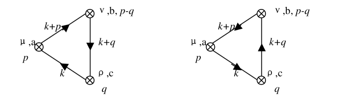
FIG. 1.: The triangle diagrams of constituent quarks.

$$S_{3}^{(\rm{normal})} = (\frac{3}{8}g^{2}-\frac{N_{c}}{16\pi^{2}})mg_{{}_{A}}^{2}\int d^{4}xTr_{f}\{\nabla_{\mu}U\nabla^{\mu}U^{{\dagger}}(\tilde{\chi}U^{{\dagger}}+U\tilde{\chi}^{{\dagger}})\}$$ (3.24)

$$+\int d^{4}x\int\frac{d^{4}p}{(2\pi)^{4}}e^{-ip\cdot x}\{-\frac{g_{{}_{A}}^{2}}{2}\alpha_{2}(p^{2})p^{\mu}Tr_{f}[\bar{V}^{\nu}(p)[\Delta_{\mu}(x),\Delta_{\nu}(x)]]$$

$$+\frac{N_{c}}{24\pi^{2}m}\alpha_{3}(p^{2})(g_{\mu\nu}p^{2}-p_{\mu}p_{\nu})Tr_{f}[\bar{V}^{\mu}(p)\bar{V}^{\nu}(x)(\xi\tilde{\chi}^{{\dagger}}\xi+\xi^{{\dagger}}\chi\xi^{{\dagger}})]$$

$$-\frac{N_{c}m}{16\pi^{2}}\kappa g_{{}_{A}}\alpha_{4}(p^{2})Tr_{f}[\bar{V}^{\mu}(p),\Delta_{\mu}(x)](\xi^{{\dagger}}\tilde{\chi}\xi^{{\dagger}}-\xi\tilde{\chi}^{{\dagger}}\xi)]$$

$$-\frac{N_{c}}{16\pi^{2}m}\kappa g_{{}_{A}}\alpha_{5}(p^{2})(g_{\mu\nu}p^{2}-p_{\mu}p_{\nu})Tr_{f}[\bar{V}^{\mu}(p),\Delta^{\nu}(x)](\xi^{{\dagger}}\tilde{\chi}\xi^{{\dagger}}-\xi\tilde{\chi}^{{\dagger}}\xi)]\}+...,$$

where the form factor $\alpha_{i}(i=2,3,4,5)$ are defined as follows,

$$\alpha_{2}(p^{2}) = g^{2}-\frac{N_{c}}{2\pi^{2}}\int_{0}^{1}dx\int_{0}^{1}dy\cdot x(1-xy)[1+\frac{m^{2}}{m^{2}-f(p^{2})}+\ln(1-\frac{f(p^{2})}{m^{2}})],$$ (3.25)

$$\alpha_{3}(p^{2}) = \int_{0}^{1}dx\frac{6x(1-x)m^{2}}{m^{2}-x(1-x)p^{2}},$$ (3.26)

$$\alpha_{4}(p^{2}) = 6\pi^{2}g^{2}-\int_{0}^{1}dx\int_{0}^{1}dy\{2x\ln(1-\frac{f(p^{2})}{m^{2}})+\frac{xy(1-x)p^{2}}{m^{2}-f(p^{2})}\},$$ (3.27)

$$\alpha_{5}(p^{2}) = \int_{0}^{1}dx\int_{0}^{1}dy\frac{2x(1-x)m^{2}}{m^{2}-f(p^{2})},$$ (3.28)

with

$$f(p^{2})=x(1-x)(1-y)p^{2}.$$ (3.29)

Moreover, the following three-point effective action with abnormal parity is related to the purpose of this present paper,

$$S_{3}^{(\rm{ab})}=\frac{iN_{c}}{2\pi^{2}}g_{{}_{A}}\epsilon^{\mu\nu\alpha\beta}\int\frac{d^{4}q_{1}}{(2\pi)^{4}}\frac{d^{4}q_{2}}{(2\pi)^{4}}\alpha_{6}(q_{1}^{2},q_{2}^{2})q_{1\mu}Tr_{f}\{\bar{V}_{\nu}(q_{1})\bar{V}_{\alpha}(q_{2})\Delta_{\beta}(q_{1}+q_{2})\}+...,$$ (3.30)

where

$$\alpha_{6}(q_{1}^{2},q_{2}^{2})=\int_{0}^{1}dx\cdot x\int_{0}^{1}dy\{1-(x+y)(1-x)(1-y)\frac{q_{1}^{2}+q_{2}^{2}}{2m^{2}}\}^{-1}$$ (3.31)

It has pointed out that, the abnormal part of these quark models including spin-1 meson usually do not pose the same symmetry as the QCD anomalous Ward identities[21], and the authors of ref.[22] have provided a method to subtract the extra terms. However, in this present paper we only focus our attention on anomalous $\rho\rightarrow\gamma\pi$ and $\omega\rightarrow\gamma\pi$ decays. Thus we have notation $\Delta_{\beta}(k)\rightarrow k_{\beta}\pi(k)$ in eq. (3.30). Using this notation we have

$$\epsilon^{\mu\nu\alpha\beta}Tr_{f}\{q_{1\mu}V_{\nu}(q_{1})\Gamma_{\alpha}(q_{2})\Delta_{\beta}(k)+q_{2\mu}V_{\nu}(q_{1})\Gamma_{\alpha}(q_{2})\Delta_{\beta}(k)\}$$ (3.32)

$$\rightarrow \epsilon^{\mu\nu\alpha\beta}eTr_{f}\{-q_{2\mu}V_{\nu}(q_{1}){\cal Q}\gamma_{\alpha}(q_{2})\Delta_{\beta}(k)+q_{1\mu}{\cal Q}\gamma_{\nu}(q_{1})V_{\alpha}(q_{2})\Delta_{\beta}(k)\}$$ (3.33)

be invariant under infinite transformation

$${\cal O}_{\mu}^{a}\rightarrow{\cal O}_{\mu}^{a}+f^{abc}{\cal O}_{\mu}^{b}\epsilon^{c},\hskip 43.36243pt{\cal O}_{\mu}=V_{\mu},\;\Delta_{\mu},$$ (3.34)

$${\cal O}_{\mu}^{0}\rightarrow{\cal O}_{\mu}^{0},\hskip 93.95122pt\gamma_{\mu}\rightarrow\gamma_{\mu}+i\partial_{\mu}\epsilon^{0},$$ (3.35)

where $\epsilon^{c},(c=1,2,...8)$ and $\epsilon^{0}$ are infinite parameters. Therefore, here no extra terms need to be subtracted.

The four-point effective action also includes both of normal parity part and abnormal parity part. Due to soft-pion theorem, the normal parity part relating to this paper reads

$$S_{4}^{({\rm normal})} = \frac{N_{c}}{192\pi^{2}}g_{{}_{A}}^{4}\int d^{4}xTr_{f}\{\nabla_{\mu}U\nabla^{\mu}U^{{\dagger}}\nabla_{\nu}U\nabla^{\nu}U^{{\dagger}}\}$$ (3.38)

$$+\frac{N_{c}}{8\pi^{2}m}g_{{}_{A}}^{2}\int d^{4}x\int\frac{d^{4}q}{(2\pi)^{4}}e^{-iq\cdot x}(g_{\mu\nu}q_{\sigma}-g_{\mu\sigma}q_{\nu}){\Big{(}}\alpha_{7}(q^{2})Tr_{f}\{\{\bar{V}^{\mu}(q),(\xi\tilde{\chi}^{{\dagger}}\xi+\xi^{{\dagger}}\chi\xi^{{\dagger}})\}\Delta^{\nu}(x)\Delta^{\sigma}(x)\}$$

$$+\alpha_{8}(q^{2})Tr_{f}\{\bar{V}^{\mu}(q)\Delta^{\nu}(x)(\xi\tilde{\chi}^{{\dagger}}\xi+\xi^{{\dagger}}\chi\xi^{{\dagger}})\Delta^{\sigma}(x)\}{\Big{)}}+...,$$

where

$$\alpha_{7}(q^{2}) = \int_{0}^{1}dx_{1}\cdot x_{1}^{2}\int_{0}^{1}dx_{2}(1-x_{2})\frac{3-2x_{1}^{2}x_{2}(1+2x_{1})(1-x_{2})q^{2}/m^{2}}{[1-x_{1}^{2}x_{2}(1-x_{2})q^{2}/m^{2}]^{2}},$$

$$\alpha_{8}(q^{2}) = \int_{0}^{1}dx_{1}\cdot x_{1}^{2}\int_{0}^{1}dx_{2}(1-x_{2})\frac{4(1-x_{1})[3-4x_{1}^{2}x_{2}(1-x_{2})q^{2}/m^{2}]}{[1-x_{1}^{2}x_{2}(1-x_{2})q^{2}/m^{2}]^{2}}.$$

For abnormal parity part, we only focus on photon to three-pseudoscalar interaction in this paper. Thus using soft-pion theorem, we have

$$S_{4}^{\gamma\rightarrow 3\Phi}=-\frac{N_{c}}{48\pi^{2}}eg_{{}_{A}}^{3}\int\frac{d^{4}q_{2}}{(2\pi)^{4}}\cdots\frac{d^{4}q_{4}}{(2\pi)^{4}}i\epsilon^{\mu\nu\alpha\beta}q_{2\nu}q_{3\alpha}q_{4\beta}A_{\mu}(q_{2}+q_{3}+q_{4})Tr_{f}\{{\cal Q}\Phi(q_{2})\Phi(q_{3})\Phi(q_{4})\},$$ (3.39)

where $\Phi$ is pseudoscalar meson fields, $A_{\mu}$ is photon field, ${\cal Q}={\rm diag}\{2/3,-1/3,-1/3\}$ is charge operator of quark fields.

So far, all meson fields in above effective actions are still non-physical. The physical pseudoscalar meson fields can be obtained via field rescaling $P\rightarrow 2F_{\pi}^{-1}P$ (here $P$ denotes pseudoscalar mesons, and we ignore the difference between $F_{\pi}$ and $F_{K}$ since we focus on $\rho$ and $\omega$ physics only). For defining physical vector meson fields, let us pay attention to kinetic term of vector mesons, which can be obtained from eq. (3.14)

$${\cal L}_{\rm kin}^{(V)}=-\frac{1}{8}g^{2}Tr_{f}\{(\partial_{\mu}V_{\nu}-\partial_{\nu}V_{\mu})(\partial^{\mu}V^{\nu}-\partial^{\nu}V^{\mu})\}+\frac{1}{4}g^{2}m_{{}_{V}}^{2}Tr_{f}\{V_{\mu}V^{\mu}\}.$$ (3.40)

Here

$$m_{{}_{V}}^{2}=\frac{m_{0}^{2}}{g^{2}}+\frac{N_{c}}{\pi^{2}g^{2}}m_{{}_{V}}^{2}\int_{0}^{1}dx\cdot x(1-x)\ln(1-\frac{x(1-x)m_{{}_{V}}^{2}}{m^{2}})$$ (3.41)

is a “common” mass parameter of vector mesons. It implies that the masses of light vector meson octet are degenerated at chiral limit and large $N_{c}$ limit. From eq. (3.40) we can see that the physical vector meson fields can be obtained via field rescaling $V_{\mu}\rightarrow g^{-1}V_{\mu}$.

C Vector meson dominant and KSRF sum rules

The direct coupling between photon and vector meson resonances is also yielded by the effects of quark loops. Therefore, when vector meson resonances are treated as bound states of constituent quarks, vector meson dominant will be yielded naturally instead of input. At the leading order of large $N_{c}$ expansion the VMD vertex reads from eq. (3.14)

$${\cal L}_{\rm VMD}=-\frac{1}{2}e\int\frac{d^{4}q}{(2\pi)^{4}}e^{-iq\cdot x}f_{\rho\gamma}^{(0)}(q^{2})(g_{\mu\nu}q^{2}-q_{\mu}q_{\nu})A^{\mu}(x)Tr_{f}\{QV^{\nu}(q)\}.$$ (3.42)

where $f_{\rho\gamma}^{(0)}(q^{2})\equiv g^{-1}\alpha_{1}(q^{2})$. At the leading order of momentum expansion, i.e., $f_{\rho\gamma}^{(0)}(q^{2}=0)$, the above equation is just the expression of VMD proposed by Sakurai[19]. In addition, at the leading order of large $N_{c}$ expansion the $V-\Phi\Phi$ vertex (where $V$ denote vector mesons and $\Phi$ denotes pseudoscalar mesons) reads from eqs. (3.14) and (3.24)

$${\cal L}_{\rm V\Phi\Phi}=-\frac{i}{4}\int\frac{d^{4}q}{(2\pi)^{4}}e^{-iq\cdot x}f_{\rho\pi\pi}^{(0)}(q^{2})(g_{\mu\nu}q^{2}-q_{\mu}q_{\nu})Tr\{V^{\mu}(q)[\Phi(x),\partial^{\nu}\Phi(x)]\},$$ (3.43)

where

$$f_{\rho\pi\pi}^{(0)}(q^{2})=\frac{1}{gF_{\pi}^{2}}[\alpha_{1}(q^{2})-g_{{}_{A}}^{2}\alpha_{2}(q^{2})]$$ (3.44)

It is well known that the KSRF(I) sum rule[23]

$$f_{\rho\gamma}(q^{2})=f_{\rho\pi\pi}(q^{2})F_{\pi}^{2}$$ (3.45)

is expected to be available at the leading order of momentum expansion. At this order we have

$$f_{\rho\gamma}^{(0)}(q^{2}=0) = g,$$ (3.46)

$$f_{\rho\pi\pi}^{(0)}(q^{2}=0) = \frac{1}{gF_{\pi}^{2}}\{g^{2}+(\frac{N_{c}}{3\pi^{2}}-g^{2})\}.$$ (3.47)

We can see that KSRF(I) sum rule is satisfied exactly for $g=\sqrt{\frac{N_{c}}{3}}\frac{1}{\pi}$. Therefore, $g=\sqrt{\frac{N_{c}}{3}}\frac{1}{\pi}$ (especially, $g\equiv\pi^{-1}$ for $N_{c}=3$) is favorite choice for the universal constant of the model.

D Low energy limit

It is well known that, at very low energy, ChPT is a rigorous consequence of the symmetry pattern of QCD and its spontaneous breaking. So that the low energy limit of those model including meson resonances must match with ChPT. The low energy limit of EMG model can be obtained via integrating over vector meson resonances. It means that, at very low energy, the dynamics of vector mesons are replaced by pseudoscalar meson fields. Since there are no interaction of vector mesons at $O(p^{2})$, at very low energy, the equation of motion $\delta{\cal L}/\delta V_{\mu}=0$ yields classics solution for vector mesons are follow

$$V_{\mu}=\frac{1}{m_{{}_{V}}^{2}}\times O(p^{3}){\rm terms},$$ (3.48)

where $p$ is momentum of pseudoscalar at very low energy. Therefore, in effective action $S_{n}$, the terms involving vector meson resonances are $O(p^{6})$ at very low energy and do not contribute to $O(p^{4})$ low energy coupling constants, $L_{i}(i=1,2,...,10)$. The low energy coupling constants $L_{i}(i\neq 7,8)$ yielded by EMG model can be directly obtained from effective actions in subsection 3.2,

$$L_{1} = \frac{1}{2}L_{2}=\frac{N_{c}}{384\pi^{2}},\hskip 57.81621ptL_{3}=-\frac{N_{c}}{64\pi^{2}}+\frac{N_{c}}{192\pi^{2}}g_{A}^{4},$$ (3.49)

$$L_{4} = L_{6}=0,\hskip 93.95122ptL_{5}=\frac{N_{c}m}{32\pi^{2}B_{0}}g_{A}^{2}$$ (3.50)

$$L_{8} = \frac{F_{0}^{2}}{128B_{0}m}(3-\kappa^{2})+\frac{3m}{64\pi^{2}B_{0}}(\frac{m}{B_{0}}-\kappa g_{A}-\frac{g_{A}^{2}}{2}-\frac{B_{0}}{6m}g_{A}^{2})+\frac{L_{5}}{2}.$$ (3.51)

$$L_{9} = \frac{N_{c}}{48\pi^{2}},\hskip 97.56493ptL_{10}=-\frac{N_{c}}{48\pi^{2}}+\frac{N_{c}}{96\pi^{2}}g_{A}^{2}.$$ (3.52)

In fact, the above expression on $L_{i}$ have been obtained in some previous refs.[5, 7, 10] (besides of $L_{8}$).

The constants $L_{7}$ has been known to get dominant contribution from $\eta_{0}$[4] and this contribution is suppressed by $1/N_{c}$. If we ignore the $\eta-\eta^{\prime}$ mixing, we have

$$L_{7}=-\frac{f_{\pi}^{2}}{128m_{\eta^{\prime}}^{2}}.$$ (3.53)

Thus the six free parameters, $g$(it has been fitted by KSRF sum rule), $g_{{}_{A}}$(it has been fitted by $n\rightarrow pe^{-}\bar{\nu}_{e}$ decay), $B_{0}$, $\kappa$, $m$ and $m_{\eta^{\prime}}$ determine all ten low energy coupling constants of ChPT. It reflects the dynamics constrains between those low energy coupling constants. Moreover, if we take $m_{u}+m_{d}\simeq 10$MeV, we can obtain $B_{0}=\frac{m_{\pi}^{2}}{m_{u}+m_{d}}\simeq 2$GeV. Then experimental values of $L_{8}$ constrains constituent quark mass $m\simeq 480$MeV (a more detail fit is in sect. IX). The numerical results for these low energy constants are in table 1.

	$L_{1}$	$L_{2}$	$L_{3}$	$L_{4}$	$L_{5}$	$L_{6}$	$L_{7}$	$L_{8}$	$L_{9}$	$L_{10}$
ChPT	$0.52\pm 0.23$	$0.72\pm 0.24$	$-2.7\pm 1.0$	$-0.3\pm 0.5$	$1.4\pm 0.5$	$-0.2\pm 0.3$	$-0.26\pm 0.15$	$0.47\pm 0.18$	$6.9\pm 0.7$	$-5.2\pm 0.3$
EMG	0.79	1.58	-4.25	0	$1.26$	0	$(-0.4\pm 0.1)^{b)}$	$0.47^{a)}$	6.33	-4.55

TABLE I.: $L_{i}$ in units of $10^{-3}$, ${\mu}=m_{\rho}$. The experimental data is from ref.[24]. a)input. b)contribution from gluon anomaly.

E Chiral expansion at $m_{\rho}$-scale

Let us calculate the on-shell decay $\rho\rightarrow\pi\pi$ and $\rho^{0}\rightarrow e^{+}e^{-}$ under the leading order of momentum expansion and under including all order information of vector meson momentum expansion respectively. Numerically, using $g_{{}_{A}}=0.75$, $g=\pi^{-1}$ and $m=480$MeV, we have

$$f_{\rho\gamma}^{(0)}(q^{2}=0)=\pi^{-1}=0.318,\hskip 57.81621ptf_{\rho\pi\pi}^{(0)}(q^{2}=0)=(0.93\times 10^{-5}){\rm MeV}^{-2},$$ (3.54)

$$f_{\rho\gamma}^{(0)}(q^{2}=m_{\rho}^{2})=0.439,\hskip 79.49744ptf_{\rho\pi\pi}^{(0)}(q^{2}=m_{\rho}^{2})=(1.14\times 10^{-5}){\rm MeV}^{-2}.$$ (3.55)

Then the decay widths are $\Gamma(\rho\rightarrow\pi\pi)=125$MeV and $\Gamma(\rho^{0}\rightarrow e^{+}e^{-})=4.35$MeV at leading order of momentum expansion, and $\Gamma(\rho\rightarrow\pi\pi)=188$MeV and $\Gamma(\rho^{0}\rightarrow e^{+}e^{-})=8.29$MeV when high order contributions of momentum expansion are included. It implies that the high order contributions of momentum expansion are very important at vector meson energy scale. Furthermore, it indicates that the chiral expansion converge slowly at vector meson energy scale. This is an important feature of chiral theory including vector meson resonances.

However, neither the results at the leading order of momentum expansion nor the results including high order contributions of vector meson momentum expansion match with experimental data, $\Gamma_{\rm exp}(\rho\rightarrow\pi\pi)=150$MeV and $\Gamma_{\rm exp}(\rho^{0}\rightarrow e^{+}e^{-})=(6.77\pm 0.32)$MeV. The reason is that, so far, the contributions from pseudoscalar meson loops are still not included. We have pointed out in introduction that these $N_{c}^{-1}$ suppression effects yield about $20\%$ contribution. Therefore, in the following sections, we will calculate the effects of pseudoscalar meson loops for various physical processes.

IV One-loop correction to $\rho$ decays

In this section we will calculate pseudoscalar one-loop correction to $\rho\rightarrow\pi\pi$ and $\rho^{0}\rightarrow e^{+}e^{-}$ decays and provide a complete prediction on these reactions. Since $m_{\pi}^{2}\ll m_{{}_{K}}^{2}<m_{\rho}^{2}$, we will treat pion as massless particle but $m_{{}_{K}}\neq 0$ in our calculation. In addition, we will omit the difference between $m_{\eta_{8}}$ and $m_{{}_{K}}$, and between $F_{\pi}$ and $F_{{}_{K}}$, since these differences are doubly suppressed by light quark mass expansion and $N_{c}^{-1}$ expansion.

A Correction to $\rho\rightarrow\pi\pi$ decay

To the next to leading order of $N_{c}^{-1}$ expansion, there are three kinds of loop diagrams of pseudoscalar mesons need to be calculated (fig.2). Recalling $m_{\pi}^{2}=0$ but $m_{\eta_{8}}^{2}=m_{{}_{K}}^{2}\neq 0$, we can see that only $K$ and $\eta_{8}$ mesons can yield non-zero contribution of tadpole diagram in fig. 2-a), since in dimensional regularization, $\int d^{D}kk^{2n}\equiv 0(n\geq-1)$. Due to the same formula, we have

$$\int d^{D}k\frac{k^{2s}}{k^{2}+m_{\varphi}^{2}+i\epsilon}\propto m_{\varphi}^{2s}\times{\rm quadratic\;divergence},\hskip 72.26999pt(s\geq 1).$$

Thus in this present paper we will ignore all contribution from quartic divergence or higher order divergences. Furthermore, in the following calculation we can find that the lowest order divergence is quadratic divergence. In means that the on-shell condition for pseudoscalar mesons and soft-pion theorem in tree level are still available even in calculation on pseudoscalar meson loops. In addition, when we calculate two-point diagram of pion, we must include all chain-like diagrams in fig. 2-c). Meanwhile, when we calculate two-point diagram of $K$ or $\eta_{8}$, we only need to calculate one-loop diagram in fig. 2-b). The reason is that the two-point diagram of pion generates a large imaginary part of ${\cal T}$-matrix for $\rho$ and $\omega$ physics, but $K$ or $\eta_{8}$ do not. If we only calculate one-loop diagram in fig. 2-b), a large error bar for phase factor will be yielded and this error will affect the study on pion-pion phase shift in section 7.

FIG. 2.: One-loop diagrams for $\rho\rightarrow\pi\pi$ decay. a)Tadpole diagram of $K$ or $\eta_{8}$. b)Two-point diagram of $K$. c)Chain-like approximation of pion.

It is convenient to evaluate pseudoscalar meson loops in terms of background field method. To expand pseudoscalar meson field around their classic solution

$$U(x)=\bar{\xi}(x)e^{i\varphi}\bar{\xi}(x),\hskip 72.26999pt\bar{U}(\Phi)=\bar{\xi}^{2}(\Phi),$$ (4.1)

where background field $\bar{U}(\Phi)$ is solution of classic motion of pseudoscalar mesons, $\delta{\cal L}/\delta U(x)=0$, $\varphi(x)$ is quantum fluctuation fields around this classic solution.

Let us first calculate the tadpole diagram (fig. 2-a). Inserting eq. (4.1) into effective action $S_{2}$ and $S_{3}$ and to retain terms including two $\Phi$ and two quantum fields $\varphi$, the $\rho-4\Phi$ vertex reads,

$${\cal L}_{\rho-4\Phi}=-\frac{1}{2F_{\pi}^{2}}\int\frac{d^{4}q}{(2\pi)^{4}}e^{-iq\cdot x}f_{\rho\pi\pi}^{(0)}(q^{2})Tr_{f}\{\rho_{\mu\nu}(q)(\partial^{\mu}\Phi\varphi\partial^{\nu}\Phi\varphi+\varphi\partial^{\mu}\Phi\partial^{\nu}\Phi\varphi-\partial^{\mu}\Phi\partial^{\nu}\Phi\{\varphi,\varphi\})\}+\cdots.$$ (4.2)

where $q$ are four-momentum of $\rho$, $\rho_{\mu\nu}(q)=q_{\mu}\rho_{\nu}(q)-q_{\nu}\rho_{\mu}(q)$, and $``\cdots^{\prime\prime}$ denotes those $\rho-4\Phi$ terms that only generate zero contribution, e.g., $Tr_{f}\{\rho_{\mu\nu}(q)\partial^{\mu}\varphi\Phi\partial^{\nu}\varphi\Phi\}$.

In terms of the completeness relation of generators $\lambda^{a}(a=1,2,\cdots,N^{2}-1)$ of $SU(N)$ group

$$Tr(\lambda^{a}A\lambda^{a}B)=-\frac{2}{N}Tr(AB)+2TrATrB,$$ (4.3)

$$Tr(\lambda^{a}A)Tr(\lambda^{a}B)=2Tr(AB)-\frac{2}{N}TrATrB,$$ (4.4)

we have

$$Tr_{f}\{\rho_{\mu\nu}(q)(\partial^{\mu}\Phi\lambda^{a}\partial^{\nu}\Phi\lambda^{a}+\lambda^{a}\partial^{\mu}\Phi\partial^{\nu}\Phi\lambda^{a}-\partial^{\mu}\Phi\partial^{\nu}\Phi\{\lambda^{a},\lambda^{a}\})\}=-4NTr_{f}\{\rho_{\mu\nu}(q)\partial^{\mu}\Phi\partial^{\nu}\Phi\}.$$ (4.5)

From viewpoint of group theory, the contribution from $K$ and $\eta_{8}$ is just one from pseudoscalar mesons in $SU(3)/SU(2)$ sector. Then tadpole diagram correction to $\rho\rightarrow\Phi\Phi$ is

$${\cal L}^{\rm(t)}_{\rho\Phi\Phi} = \frac{i}{4}\int\frac{d^{4}q}{(2\pi)^{4}}e^{-iq\cdot x}f_{\rho\pi\pi}^{(0)}(q^{2})(g_{\mu\nu}q^{2}-q_{\mu}q_{\nu})Tr_{f}\{\rho^{\mu}(q)[\Phi(x),\partial^{\nu}\Phi(x)]\}\int\frac{d^{4}k}{(2\pi)^{4}}\frac{4iF_{\pi}^{-2}}{k^{2}-m_{{}_{K}}^{2}+i\epsilon}$$ (4.6)

$$= \frac{i}{4}\frac{\lambda m_{{}_{K}}^{2}}{4\pi^{2}F_{\pi}^{2}}\int\frac{d^{4}q}{(2\pi)^{4}}e^{-iq\cdot x}f_{\rho\pi\pi}^{(0)}(q^{2})(g_{\mu\nu}q^{2}-q_{\mu}q_{\nu})Tr_{f}\{\rho^{\mu}(q)[\Phi(x),\partial^{\nu}\Phi(x)]\},$$ (4.7)

where $\lambda$ is a constant absorbing quadratic divergence from meson loops

$$\lambda=(\frac{4\pi\mu^{2}}{m^{2}})^{\epsilon/2}\Gamma(1-\frac{D}{2}).$$ (4.8)

In the following we will calculate the two-point diagram(TPD) of pseudoscalar mesons. The leading order $\rho\Phi\Phi$ vertex of $N_{c}^{-1}$ expansion has been given in eq. (3.43). Here we need to further obtain explicit 4-$\Phi$ vertex from the effective actions of section 3. Inserting eq. (4.1) into $S_{2}$, $S_{3}^{\rm(normal)}$ and $S_{4}^{\rm(normal)}$ and retaining terms with two $\Phi$ and two $\varphi$ fields, we have

$${\cal L}_{4\Phi} = \frac{1}{2}\int\frac{d^{4}q}{(2\pi)^{4}}e^{-iq\cdot x}[g_{\mu\nu}+\frac{N_{c}}{4F_{\pi}^{2}}(g^{2}-\frac{g_{{}_{A}}^{4}}{3\pi^{2}})(g_{\mu\nu}q^{2}-q_{\mu}q_{\nu})]Tr_{f}\{\tilde{\Gamma}^{\mu}(q)[\varphi(x),\partial^{\nu}\varphi(x)]\}$$ (4.10)

$$+\cdots,$$

with

$$\tilde{\Gamma}_{\mu}=\frac{1}{2F_{\pi}^{2}}[\Phi,\partial_{\mu}\Phi].$$ (4.11)

Here $``\cdots^{\prime\prime}$ denotes that those 4-$\Phi$ terms only yield zero contribution due to transveral operator $g_{\mu\nu}q^{2}-q_{\mu}q_{\nu}$ in $V-\Phi\Phi$ vertex, such as $Tr_{f}\{[\partial_{\mu}\Phi,\varphi][\partial^{\mu}\Phi,\varphi]\}$. Then two-point diagram correction to $\rho\Phi\Phi$ vertex is

$${\cal L}_{\rho\Phi\Phi}^{\rm(TPD)} = \frac{1}{16F_{\pi}^{2}}\int\ frac{d^{4}q}{(2\pi)^{4}}f_{\rho\pi\pi}^{(0)}(q^{2})(g_{\mu\nu}q^{2}-q_{\mu}q_{\nu})[g_{\alpha\beta}+\frac{3}{4F_{\pi}^{2}}(g^{2}-\frac{g_{{}_{A}}^{4}}{3\pi^{2}})(g_{\alpha\beta}q^{2}-q_{\alpha}q_{\beta})]Tr_{f}\{\rho^{\mu}(q)[\lambda^{a},\lambda^{b}]\}$$ (4.13)

$$\times Tr_{f}\{[\Phi(x),\partial^{\alpha}\Phi(x)][\lambda^{a},\lambda^{b}]\}\int\frac{d^{4}k}{(2\pi)^{4}}\frac{ik^{\nu}}{k^{2}-m_{\varphi}^{2}+i\epsilon}\frac{i(2k+q)^{\beta}}{(k+q)^{2}-m_{\varphi}^{2}+i\epsilon}.$$

Using completeness relation of generators of $SU(N)$ group (4.3), we have

$$Tr\{A[\lambda^{a},\lambda^{b}]\}Tr\{B[\lambda^{a},\lambda^{b}]\}=-8NTr(AB)+8TrATrB.$$ (4.14)

Then taking $N=2$, we obtain $SU(2)$ (pion meson) correction as follow

$${\cal L}_{\rm V\Phi\Phi}^{\rm TPD}[SU(2)]=\frac{i}{4}\int\frac{d^{4}q}{(2\pi)^{4}}e^{-iq\cdot x}f_{\rho\pi\pi}^{(0)}(q^{2})\Sigma_{\pi}(q^{2})(g_{\mu\nu}q^{2}-q_{\mu}q_{\nu})Tr\{V^{\mu}(q)[\Phi(x),\partial^{\nu}\Phi(x)]\},$$ (4.15)

where

$$\Sigma_{\pi}(q^{2}) = \frac{q^{2}}{4\pi^{2}F_{\pi}^{2}}[1+\frac{3q^{2}}{4F_{\pi}^{2}}(g^{2}-\frac{g_{{}_{A}}^{4}}{3\pi^{2}})]\{\frac{\lambda}{6}+\int_{0}^{1}dx\cdot x(1-x)\ln{\frac{x(1-x)q^{2}}{m_{{}_{K}}^{2}}}$$ (4.17)

$$+\frac{i}{6}Arg(-1)\theta(q^{2}-4m_{\pi}^{2})(1-\frac{4m_{\pi}^{2}}{q^{2}})^{3/2}\},$$

with

$$Arg(-1) = (1+2k)\pi,\hskip 50.58878ptk=0,\pm 1,\pm 2,\cdots,$$ (4.18)

$$\theta(x-y) = \left\{1,\hskip 79.49744ptx>y;\atop 0,\hskip 79.49744ptx\leq y.\right.$$ (4.19)

In eq. (4.17), the phase factor $(1-4m_{\pi}^{2}/q^{2})^{3/2}$ denotes the pion mass correction, which is yielded by unitarity of $S$-matrix(see section 5). In addition, taking $N=3-2$ in eq. (4.14), we can obtain $SU(3)/SU(2)$ ($K$-meson) correction

$${\cal L}_{\rm V\Phi\Phi}^{\rm TPD}[SU(3)/SU(2)]=-\frac{i}{4}\int\frac{d^{4}q}{(2\pi)^{4}}e^{-iq\cdot x}f_{\rho\pi\pi}^{(0)}(q^{2})\Sigma_{K}(q^{2})(g_{\mu\nu}q^{2}-q_{\mu}q_{\nu})Tr\{V^{\mu}(q)[\Phi(x),\partial^{\nu}\Phi(x)]\},$$ (4.20)

where

$$\Sigma_{K}(q^{2})=\frac{m_{{}_{K}}^{2}}{8\pi^{2}F_{\pi}^{2}}[1+\frac{3q^{2}}{4F_{\pi}^{2}}(g^{2}-\frac{g_{{}_{A}}^{4}}{3\pi^{2}})]\{\lambda(1-\frac{q^{2}}{6m_{{}_{K}}^{2}})+\int_{0}^{1}dx(1-\frac{x(1-x)q^{2}}{m_{{}_{K}}^{2}})\ln(1-\frac{x(1-x)q^{2}}{m_{{}_{K}}^{2}})\}.$$ (4.21)

Comparing eq. (4.15) with eq. (3.43), we can see that every two-point loop in chain-like approximation (fig. 2-c) contributes a factor $-\Sigma_{\pi}(q^{2})$. Therefore, to sum over all diagrams in fig. 2-c), we obtain

$${\cal L}_{\rm V\Phi\Phi}^{\pi-{\rm loop}}=-\frac{i}{4}\int\frac{d^{4}q}{(2\pi)^{4}}e^{-iq\cdot x}\frac{f_{\rho\pi\pi}^{(0)}(q^{2})}{1+\Sigma_{\pi}(q^{2})}(g_{\mu\nu}q^{2}-q_{\mu}q_{\nu})Tr\{V^{\mu}(q)[\Phi(x),\partial^{\nu}\Phi(x)]\}.$$ (4.22)

Eq. (4.22) together with eqs. (4.6) and (4.18) lead to “complete” $\rho-\pi\pi$ vertex to the next to leading order of $N_{c}^{-1}$ expansion,

$${\cal L}_{\rho\pi\pi}^{(c)}=-\frac{i}{4}\int\frac{d^{4}q}{(2\pi)^{4}}e^{-iq\cdot x}f_{\rho\pi\pi}^{(c)}(q^{2})(g_{\mu\nu}q^{2}-q_{\mu}q_{\nu})Tr\{\rho^{\mu}(q)[\pi(x),\partial^{\nu}\pi(x)]\},$$ (4.23)

where

$$f_{\rho\pi\pi}^{(c)}(q^{2})=f_{\rho\pi\pi}^{(0)}(q^{2})(\frac{1}{1+\Sigma_{\pi}(q^{2})}+\Sigma_{K}(q^{2})-\frac{\lambda m_{{}_{K}}^{2}}{4\pi^{2}F_{\pi}^{2}}).$$ (4.24)

B Correction to $\rho\rightarrow e^{+}e^{-}$ decay

To the next to leading order of $N_{c}^{-1}$ expansion, we need consider three kinds of loop diagrams of pseudoscalar mesons correction to VMD vertex (fig.3).

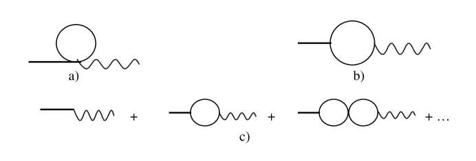
FIG. 3.: One-loop diagrams for $\rho^{0}-\gamma$ mixing. a)Tadpole diagram of $K$ or $\eta_{8}$. b)Two-point diagram of $K$. c)Chain-like approximation of pion.

We first evaluate the tadpole contribution in fig.3-a). Inserting eq. (4.1) into $S_{2}$, we obtain $\rho\gamma\varphi\varphi$ vertex as follow

$${\cal L}_{\rho\gamma\varphi\varphi}=\frac{1}{F_{\pi}^{2}}e\int\frac{d^{4}q}{(2\pi)^{4}}e^{-iq\cdot x}f_{\rho\gamma}^{(0)}(q^{2})(g_{\mu\nu}q^{2}-q_{\mu}q_{\nu})A^{\mu}(x)Tr_{f}\{\rho^{\nu}(q)(\frac{1}{2}{\cal Q}\{\varphi,\varphi\}-\varphi{\cal Q}\varphi)\}.$$ (4.25)

Then the tadpole correction of $K$ or $\eta_{8}$ mesons to VMD vertex is

$${\cal L}_{\rm VMD}^{(t)}=\frac{1}{2}\frac{\lambda m_{{}_{K}}^{2}}{8\pi^{2}F_{\pi}^{2}}e\int\frac{d^{4}q}{(2\pi)^{4}}e^{-iq\cdot x}f_{\rho\gamma}^{(0)}(q^{2})(g_{\mu\nu}q^{2}-q_{\mu}q_{\nu})A^{\mu}(x)Tr_{f}\{{\cal Q}\rho^{\nu}(q)\}.$$ (4.26)

For calculating contribution of fig. 3-b) and fig. 3-c), the $\gamma-\varphi\varphi$ vertex is necessary

$${\cal L}_{\gamma\varphi\varphi}=-\frac{i}{2}e\int\frac{d^{4}q}{(2\pi)^{4}}e^{-iq\cdot x}[1+\frac{g}{2}f_{\rho\pi\pi}^{(0)}(q^{2})(g_{\mu\nu}q^{2}-q_{\mu}q_{\nu})]A^{\mu}(q)Tr_{f}\{{\cal Q}[\varphi(x),\partial^{\nu}\varphi(x)]\}.$$ (4.27)

Calculations on fig. 3-b) and fig. 3-c) are similar to one on fig. 2. The final result on “complete” VMD vertex is

$${\cal L}_{\rho\gamma}^{(c)}=-\frac{1}{2}e\int\frac{d^{4}q}{(2\pi)^{4}}e^{-iq\cdot x}f_{\rho\gamma}^{(c)}(q^{2})(g_{\mu\nu}q^{2}-q_{\mu}q_{\nu})A^{\mu}(x)Tr_{f}\{{\cal Q}\rho^{\nu}(q)\},$$ (4.28)

where

$$f_{\rho\gamma}^{(c)}(q^{2})=f_{\rho\gamma}^{(0)}(q^{2})(1-\frac{\lambda m_{{}_{K}}^{2}}{8\pi^{2}F_{\pi}^{2}})-f_{\rho\pi\pi}^{(0)}(q^{2})[\frac{\Sigma_{\pi}^{\gamma}(q^{2})}{1+\Sigma_{\pi}(q^{2})}-\Sigma_{K}^{\gamma}(q^{2})],$$ (4.29)

with

$$\Sigma_{\pi}^{\gamma}(q^{2}) = \frac{q^{2}}{4\pi^{2}}[1+\frac{g}{2}q^{2}f_{\rho\pi\pi}^{(0)}(q^{2})]\{\frac{\lambda}{6}+\int_{0}^{1}dx\cdot x(1-x)\ln{\frac{x(1-x)q^{2}}{m_{{}_{K}}^{2}}}$$ (4.31)

$$+\frac{i}{6}Arg(-1)\theta(q^{2}-4m_{\pi}^{2})(1-\frac{4m_{\pi}^{2}}{q^{2}})^{3/2}\},$$

$$\Sigma_{K}^{\gamma}(q^{2}) = \frac{m_{{}_{K}}^{2}}{8\pi^{2}}[1+\frac{g}{2}q^{2}f_{\rho\pi\pi}^{(0)}(q^{2})]\{\lambda(1-\frac{q^{2}}{6m_{{}_{K}}^{2}})+\int_{0}^{1}dx(1-\frac{x(1-x)q^{2}}{m_{{}_{K}}^{2}})\ln(1-\frac{x(1-x)q^{2}}{m_{{}_{K}}^{2}})\}.$$ (4.32)

C Cancellation of divergence

From the above calculations we can find that only quadratic divergence appears in one-loop contribution of pseudoscalar mesons. Since the present model is a non-renormalizable effective theory, the divergences have to be factorized, i.e., the parameter $\lambda$ has to be determined phenomenologically.

The on-shell decay $\phi\rightarrow\pi\pi$ is forbidden by G parity conservation and Zweig rule. Experiment also show that branching ratios of this decay is very small, $B(\phi\rightarrow\pi\pi)=(8\;{+5\atop-4})\times 10^{-5}$. Theoretically, this decay can occur through photon-exchange or $K$-loop(fig. 4). The latter two diagrams yield non-zero imaginary part of decay amplitude. Thus the real part yielded by the latter two diagrams must be very small. We can determine $\lambda$ due to this requirement. From the calculation in the above two subsection, we see that result yielded by the latter two diagrams is proportional to a factor

$$\lambda(\frac{p^{2}}{6}-m_{{}_{K}}^{2})-\int_{0}^{1}dx\cdot[m_{{}_{K}}^{2}-x(1-x)p^{2}]\ln{(1-\frac{x(1-x)p^{2}}{m_{{}_{K}}^{2}})}.$$ (4.33)

Then Zweig rule requires

$$\{\lambda(\frac{p^{2}}{2}-m_{{}_{K}}^{2})-Re\int_{0}^{1}dx\cdot[m_{{}_{K}}^{2}-x(1-x)p^{2}]\ln{(1-\frac{x(1-x)p^{2}}{m_{{}_{K}}^{2}})}\}|_{p^{2}=m_{\phi}^{2}}\simeq 0.$$ (4.34)

Form the above equation, we obtain

$$\lambda\simeq 0.54.$$ (4.35)

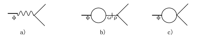
FIG. 4.: Some diagrams for $\phi\rightarrow\pi\pi$ decay. The one-loop in figure b) and c) is $K$-loop.

D Numerical results

The momentum-dependent widths for $\rho\rightarrow\pi\pi$ and $\rho\rightarrow e^{+}e^{-}$ can be obtained from the “complete” vertices (4.23) and (4.28),

$$\Gamma_{\rho\rightarrow\pi\pi}(q^{2}) = \frac{|f_{\rho\pi\pi}^{(c)}(q^{2})|^{2}q^{4}}{48\pi}\sqrt{q^{2}}(1-\frac{4m_{\pi}^{2}}{q^{2}})^{3/2},$$ (4.36)

$$\Gamma_{\rho\rightarrow e^{+}e^{-}}(q^{2}) = \frac{\pi\alpha_{\rm e.m.}^{2}}{3}|f_{\rho\gamma}^{(c)}(q^{2})|^{2}\sqrt{q^{2}}.$$ (4.37)

Inputting $m=480$MeV, $g_{{}_{A}}=0.75$, $g=\pi^{-1}$, $\lambda=0.54$ and $\sqrt{q^{2}}=m_{\rho}=770$MeV, we obtain the on-shell decay widths

$$\Gamma(\rho\rightarrow\pi\pi)=146.4{\rm MeV},$$ (4.38)

$$\Gamma(\rho\rightarrow e^{+}e^{-})=6.98{\rm KeV}.$$ (4.39)

These results agree with experimental data, $150$MeV and $(6.77\pm 0.32)$KeV, excellently. It also implies that the one-loop diagrams of pseudoscalar mesons yield significant contribution at vector meson energy scale.

E Loop correction to $\gamma\rightarrow\pi\pi$ vertex

Here we will further calculate loop correction of pseudoscalar mesons to $\gamma\rightarrow\pi\pi$ vertex, which is needed by studies in the following section.

The calculation of loop correction to $\gamma\rightarrow\pi\pi$ vertex is similar to one to $\rho\rightarrow\pi\pi$ vertex (fig. 5). The $\gamma\Phi\Phi$ vertex and 4-$\Phi$ vertex has given in eqs. (4.27) and (4.10) respectively. Here $\gamma$ to 4-$\Phi$ vertex is further needed for evaluating the tadpole contribution in fig. 2-a),

$${\cal L}_{\gamma-4\Phi} = -\frac{i}{2F_{\pi}^{2}}eA_{\mu}Tr_{f}\{[[{\cal Q},\Phi],\varphi][\partial^{\mu}\Phi,\varphi]\}-\frac{i}{F_{\pi}^{2}}e\int\frac{d^{4}q}{(2\pi)^{4}}e^{-iq\cdot x}gf_{\rho\pi\pi}^{(0)}(q^{2})(q^{2}g_{\mu\nu}-q_{\mu}q_{\nu})A^{\mu}(q)$$ (4.41)

$$\times Tr_{f}\{{\cal Q}(\Phi\varphi\partial^{\nu}\Phi\varphi+\varphi\Phi\partial^{\nu}\Phi\varphi+\varphi\Phi\varphi\partial^{\nu}\Phi-\frac{3}{2}\Phi\partial^{\nu}\Phi\{\varphi,\varphi\}\}.$$

Then due to conservation of electromagnetic current, the “complete” $\gamma\rightarrow\pi\pi$ is

$${\cal L}_{\gamma\pi\pi}^{(c)}=\frac{1}{2}\int\frac{d^{4}q}{(2\pi)^{4}}e^{-iq\cdot x}e\bar{F}_{\gamma\pi\pi}(q^{2})A_{\mu}(q)Tr_{f}\{{\cal Q}[\pi,\partial^{\mu}\pi]\},$$ (4.42)

where $\bar{F}_{\gamma\pi\pi}(q^{2})$ is nonresonant background part of pion form factor,

$$\bar{F}_{\gamma\pi\pi}(q^{2}) = \frac{1}{1+\Sigma_{\pi}(q^{2})}+\Sigma_{K}(q^{2})-\frac{\lambda m_{{}_{K}}^{2}}{8\pi^{2}F_{\pi}^{2}}+\frac{g}{2}q^{2}f_{\rho\pi\pi}^{(0)}(q^{2})(\frac{1}{1+\Sigma_{\pi}(q^{2})}+\Sigma_{K}(q^{2})-\frac{3\lambda m_{{}_{K}}^{2}}{8\pi^{2}F_{\pi}^{2}})$$ (4.44)

$$-\frac{3q^{2}}{4F_{\pi}^{2}}(g^{2}-\frac{g_{{}_{A}}^{4}}{3})[1+\frac{3q^{2}}{4F_{\pi}^{2}}(g^{2}-\frac{g_{{}_{A}}^{4}}{3})]^{-1}(\frac{\Sigma_{\pi}(q^{2})}{1+\Sigma_{\pi}(q^{2})}-\Sigma_{k}(q^{2})).$$

Since $\Sigma_{K}(q^{2})-\lambda m_{{}_{K}}^{2}/(8\pi^{2}F_{\pi}^{2})$ is $O(q^{2})$, $\bar{F}_{\gamma\pi\pi}(q^{2}=0)=1$ is still satisfied. It means that this loop correction does not break $U(1)_{\rm e.m.}$ gauge invariance.

V Unitarity and Large $N_{c}$ Expansion

The unitarity of $S$-matrix, or optical theorem

$${\rm Im}{\cal T}_{\beta,\alpha}=\frac{1}{2}\sum_{\rm all\;\gamma}{\cal T}_{\gamma,\alpha}{\cal T}_{\gamma,\beta}^{*},$$ (5.1)

has to be satisfied for any well-defined quantum field theory, where the ${\cal T}_{\beta,\alpha}$ transition amplitude, and $\gamma$ denotes all possible intermediate states on mass shells. It is well-known that a low energy effective meson theory should be a well-defined perturbative theory in $N_{c}^{-1}$ expansion[17]. Therefore, we can expand ${\cal T}$-matrix in powers of $N_{c}^{-1}$ expansion,

$${\cal T}=\sum_{n=0}^{\infty}{\cal T}_{n},\hskip 72.26999pt{\cal T}_{n}\sim O((\sqrt{N_{c}})^{-n}).$$ (5.2)

Then the unitarity of $S$-matrix for a low energy effective meson theory can be proved order by order in powers of $N_{c}^{-1}$ expansion,

$${\rm Im}({\cal T}_{\beta,\alpha})_{n}=\frac{1}{2}\sum_{\rm all\;\gamma}\sum_{m\leq n}({\cal T}_{\gamma,\alpha})_{m}({\cal T}_{\gamma,\beta}^{*})_{n-m}.$$ (5.3)

In this present paper, we will discuss the unitarity of $S$-matrix of several chiral quark model at vector meson energy scale. In particular, as an example, we will directly examine unitarity in EMG model via forward scattering of $\rho$-meson.

From effective action $S_{2}$, we can see that $F_{\pi}$ and $g$ are both $O(\sqrt{N_{c}})$. So that every meson external line is $O(1/\sqrt{N_{c}})$ and every meson internal line is $O(1/N_{c})$. In addition, from effective action $S_{n}$ we also see that every vertex is $O(N_{c})$. Therefore, any transition amplitudes with $n_{{}_{V}}$ vertex, $n_{e}$ external meson lines, $n_{i}$ internal meson lines and $n_{l}$ loops of mesons are order

$$N_{c}^{1-n_{l}-n_{e}/2},$$ (5.4)

where relation $n_{l}=n_{i}-n_{{}_{V}}+1$ has been used.

Using the above power counting rule, we can obtain a well-known fact that unitarity of $S$-matrix requires that on-shell transition amplitude from a vector meson to any meson states must be real at the leading order of $N_{c}^{-1}$ expansion.

From eq. (3.44), we can see that, at the leading order of $N_{c}^{-1}$ expansion, the on-shell $\rho\rightarrow\pi\pi$ transition amplitude is proportional to $f_{\rho\pi\pi}^{(0)}(m_{\rho}^{2})$. Thus the above theorem requires $\alpha_{1}(m_{\rho}^{2})$ and $\alpha_{2}(m_{\rho}^{2})$ defined in eqs. (3.15) and (3.25) are real. In the other words, it means that, in chiral quark model including vector meson resonances, the unitarity of $S$-matrix requires constituent quark mass ${\bf m>m_{\rho}/2}$. In fact, this point is insured in EMG model by $m\simeq 480$MeV which is fitted by low energy limit of the model. However, in many other version of chiral quark model[7, 8, 9, 20], the constituent quark mass are constrained around 300MeV. Obviously, this value does not yield unitarity $S$-matrix for single-vector meson processes, since all form factor defined in section 3, $\alpha_{i}(q^{2})$, are not real for $q^{2}\sim m_{\rho}^{2}$. It also means that, in those model, the chiral expansion at vector meson energy scale is not convergent.

In the following we will explicitly examine the eq. (5.1) in forward scattering of $\rho-$meson up to three-loop level of mesons. The examination on other processes can be performed similarly. For $\alpha=\beta=\rho$ in eq. (5.1), $<\gamma|=<\pi\pi|$ is dominant. The for forward scattering of $\rho$-meson, eq. (5.1) becomes

$$\frac{2}{(2\pi)^{4}}{\rm Im}{\cal T}_{\rho,\rho}=\Gamma(\rho\rightarrow\pi\pi)=\frac{|f_{\rho\pi\pi}^{(c)}(m_{\rho}^{2})|^{2}m_{\rho}^{5}}{48\pi}(1-\frac{4m_{\pi}^{2}}{m_{\rho}})^{3/2}.$$ (5.5)

The both of ${\cal T}_{\rho,\rho}$ and $f_{\rho\pi\pi}^{(c)}$ can be expanded in series of $N_{c}^{-1}$ expansion,

$${\cal T}_{\rho,\rho}=\sum_{n=0}^{\infty}({\cal T}_{\rho,\rho})_{2n}\hskip 72.26999ptf_{\rho\pi\pi}^{(c)}=\sum_{n=0}^{\infty}(f_{\rho\pi\pi}^{(c)})_{2n+1}.$$ (5.6)

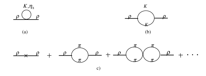
FIG. 5.: One-loop diagrams correcting to $\rho$ propagator. a)Tadpole diagram of $K$ or $\eta_{8}$. b)Two-point diagram of $K$. c)Chain-like approximation of pion.

At the leading order, Im$({\cal T}_{\rho,\rho})_{0}=0$ is obviously satisfied. For obtaining the imaginary part of $({\cal T}_{\rho,\rho})_{2}$, we need to calculate meson loop correction in fig. 5. The calculations are similar to one in section (IV.B), and the result is

$${\cal L}_{\rho\rho}^{1-loop}=\frac{1}{2}\int\frac{d^{4}q}{(2\pi)^{4}}e^{-iq\cdot x}[f_{\rho\pi\pi}^{(0)}(q^{2})]^{2}\{\frac{q^{4}\Sigma_{\pi}^{(0)}(q^{2})}{1+\Sigma_{\pi}(q^{2})}-q^{2}m_{{}_{K}}^{2}\Sigma_{K}^{(0)}(q^{2})\}(g_{\mu\nu}q^{2}-q_{\mu}q_{\nu})\rho_{i}^{\mu}(q)\rho_{i}^{\nu}(x),$$ (5.7)

where

$$\Sigma_{\pi}^{(0)}(q^{2}) = \frac{1}{8\pi^{2}}\{\frac{\lambda}{6}+\int_{0}^{1}dx\cdot x(1-x)\ln{\frac{x(1-x)q^{2}}{m_{{}_{K}}^{2}}}+\frac{i}{6}Arg(-1)\theta(q^{2}-4m_{\pi}^{2})(1-\frac{4m_{\pi}^{2}}{q^{2}})^{3/2}\},$$ (5.8)

$$\Sigma_{K}^{(0)}(q^{2}) = \frac{1}{16\pi^{2}}\{\lambda(1-\frac{q^{2}}{6m_{{}_{K}}^{2}})+\int_{0}^{1}dx(1-\frac{x(1-x)q^{2}}{m_{{}_{K}}^{2}})\ln(1-\frac{x(1-x)q^{2}}{m_{{}_{K}}^{2}})\}.$$ (5.9)

Then taking $Arg(-1)=-\pi$, we obtain

$$\frac{2}{(2\pi)^{4}}{\rm Im}({\cal T}_{\rho,\rho})_{2}=\frac{[f_{\rho\pi\pi}^{(0)}(m_{\rho}^{2})]^{2}m_{\rho}^{5}}{48\pi}(1-\frac{4m_{\pi}^{2}}{m_{\rho}})^{3/2}.$$ (5.10)

Noting that $(f_{\rho\pi\pi}^{(c)})_{1}=f_{\rho\pi\pi}^{(0)}$, we can see the eq. (5.5) is satisfied at the next to leading order.

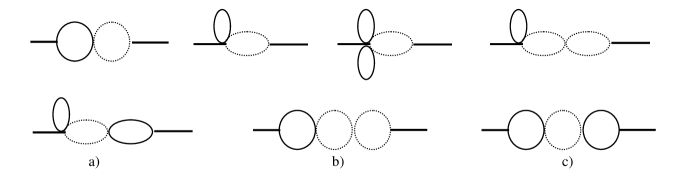
FIG. 6.: Two-loop and three-loop diagrams correcting to $\rho$ propagator. Here loops with solid line denote $K$ or $\eta_{8}$ loops, and loops with dash line denote pion loops. It should be pointed out that in fig. a), b) and c), the positions of pion loop and $K$ loop can exchange.

If the two-loop diagrams and three-loop diagrams in fig. 6 are further considered, we can prove the eq. (5.5) is satisfied up to $O(N_{c}^{-3})$. The details of calculation are omitted here.

Finally, eq. (5.5) also tell us that the “complete” propagator of $\rho$-meson is

$$\Delta_{\mu\nu}^{(\rho)}(q^{2})=\frac{-i}{q^{2}-\tilde{m}_{\rho}^{2}+i\sqrt{q^{2}}\Gamma_{\rho}(q^{2})}(g_{\mu\nu}-(\propto\frac{q_{\mu}q_{\nu}}{m_{\rho}^{2}})\;{\rm term}),$$ (5.11)

where $\Gamma_{\rho}(q^{2})=\Gamma_{\rho\rightarrow\pi\pi}(q^{2})$ given in eq. (4.36). Since vector meson is treated at tree level, the $(\propto q_{\mu}q_{\nu}/m_{\rho}^{2})$ term in propagator is unimportant. Then propagator (5.11) is just well-known Breit-Wigner formula for spin-1 resonances.

Because the width in $\rho$-resonance (possessing a complex pole) propagator (5.11) is momentum-dependent, it must be addressed that the mass parameter $\tilde{m}_{\rho}$ is not the physical mass $m_{\rho}=770$MeV. Let us interpret this point briefly. Empirically, the physical mass of resonance is defined as position of pole(real value) in relevant scattering cross section, or theoretically, it should be defined as real part of complex pole possessed by resonance. It is well-known that the width of $\rho$-resonance is generated by pion loops. For a simple VMD model, the leading order of $\rho-\pi\pi$ coupling is independent of $q^{2}$. Thus one has $\Gamma_{\rho}^{(VMD)}(q^{2})\propto\sqrt{q^{2}}$, and due to equation

$$q^{2}-\tilde{m}_{\rho}^{2}+i\frac{\Gamma_{\rho}}{m_{\rho}}q^{2}=0,$$ (5.12)

we obtain the complex pole of $\rho$-resonance is $q^{2}=m_{\rho}^{2}(1-i\epsilon+O(\epsilon^{2}))$ with $\epsilon=\Gamma_{\rho}/m_{\rho}\simeq 0.19$. The result yields $\tilde{m}_{\rho}=m_{\rho}\sqrt{1+\epsilon^{2}}=784$MeV. In particular, in the WCCWZ realization for vector meson fields used by this paper, $\rho-\pi\pi$ coupling is proportional to $q^{2}$ at least. Hence one has $\Gamma_{\rho}(q^{2})\propto q^{4}\sqrt{q^{2}}$ at least, and complex pole equation

$$q^{2}-\tilde{m}_{\rho}^{2}+i\frac{\Gamma_{\rho}}{m_{\rho}^{5}}q^{6}=0.$$ (5.13)

It yields $\tilde{m}_{\rho}=m_{\rho}\sqrt{1+3\epsilon^{2}}=810$MeV, which poses a significant correction.

The above discussions imply that: 1) For resonance with large width, the mass parameter in its propagator is different from its physical mass. The correction is proportional to the ratio of resonant width to physical mass. 2) The mass in the original effective lagrangian only emerges as a parameter instead of a physical quantity measured directly in experiment. 3) The choice of mass parameter is relied on the choice of model. But the physical quantity must be independent of this choice.

Since in our result all hadronic couplings include all order information of the chiral perturbative expansion and one-loop effects of pseudoscalar mesons, the momentum-dependence of $\Gamma_{\rho}(q^{2})$ is very complicate. It is difficult to determine $\tilde{m}_{\rho}$ via the above method. The prediction on $\tilde{m}_{\rho}$ will be found in section VII.

VI $\rho^{0}-\omega$ Mixing and $\omega\rightarrow\pi^{+}\pi^{-}$ decay

The investigation of $\rho^{0}-\omega$ mixing, which is considered as the important source of charge symmetry breaking[25] in nuclear physics, has been an active subject[26]-[36]. The mixing amplitude for on-mass-shell of vector mesons has been observed directly in the measurement of the pion form-factor in the time-like region from the process $e^{+}e^{-}\rightarrow\pi^{+}\pi^{-}$[29, 37]. For roughly twenty years, $\rho^{0}-\omega$ mixing amplitude was assumed constant or momentum independent even if $\rho$ and $\omega$ have the space-like momenta, far from the on-shell point. Several years ago, this assumption was firstly questioned by Goldman et. al.[32], and the mixing amplitude was found to be significantly momentum dependent within a simple quark loop model. Subsequently, various authors have argued such momentum dependence of the $\rho^{0}-\omega$ mixing amplitude by using various approaches[33, 34]. In particular, the authors of ref.[34] has pointed out that $\rho^{0}-\omega$ mixing amplitude must vanish at $q^{2}=0$(where $q^{2}$ denotes the four-momentum square of the vector mesons) within a broad class of model. This point will be also examined in EMG model.

In the most recent references[26, 27, 28], the $\omega\rightarrow\pi^{+}\pi^{-}$ decay was treated as being dominant via $\rho$-resonance exchange, and the direct $\omega\pi^{+}\pi^{-}$ coupling is neglected. It has been pointed out in ref.[30] that the neglect of $\omega$ “direct” coupling to $\pi^{+}\pi^{-}$ is not valid. It can be naturally understood since $\pi\pi$ can make up of vector-isovector system, whose quantum numbers are same to $\rho$ meson. Thus in an effective lagrangian based on chiral symmetry, every $\rho$ field can be replaced by $\pi\pi$ and does not conflict with symmetry. Although authors of ref.[30] also pointed out that the present experimental data still can not be used to separate “direct” $\omega\pi\pi$ coupling from $\omega-\rho$ mixing contribution in model-independent way, it is very interesting to perform a theoretical investigation on “direct” $\omega\pi\pi$ coupling contribution.

It has been known that $\omega\rightarrow\pi^{+}\pi^{-}$ decay amplitude receive the contribution from two sources: isospin symmetry breaking due to $u-d$ quark mass difference and electromagnetic interaction. In section 3 we have shown that VMD in meson physics is natural consequence of the present formalism instead of input. The $\rho\rightarrow e^{+}e^{-}$ decays are also predicted successfully. Therefore, the dynamics of electromagnetic interactions of mesons has been well established, and the calculation for $\omega\rightarrow\pi^{+}\pi^{-}$ decay from the transition $\omega\rightarrow\gamma\rightarrow\rho\rightarrow\pi\pi$ and “direct” $\omega\rightarrow\gamma\rightarrow\pi\pi$ is straightforward. Then we can determine isospin breaking parameter $\delta m_{q}\equiv m_{d}-m_{u}$ via $\omega\rightarrow\pi^{+}\pi^{-}$ decay. This parameter is urgently wanted by determination of light quark mass ratios.

A Relevant effective vertices at tree level

Here we first abstract those vertices relating to $\omega\rightarrow\pi\pi$ decay from effective action in section III.

The $\rho^{0}-\omega$ mixing vertex, which breaks isospin symmetry, is included in eq. (3.24),

$${\cal L}_{\omega\rho}^{(0)}=\frac{N_{c}}{6\pi^{2}g^{2}}\frac{m_{u}-m_{d}}{m}\int\frac{d^{4}q}{(2\pi)^{4}}e^{-iq\cdot x}\alpha_{3}(q^{2})(g_{\mu\nu}q^{2}-q_{\mu}q_{\nu})\omega^{\mu}(q)\rho^{0\nu}(x)+O((m_{d}-m_{u})^{2}).$$ (6.1)

The isospin symmetry unbroken vertex-$\Phi\Phi$ vertex (including $\rho\pi\pi$, $\Delta I=0$ $\rho KK$ and $\omega KK$ vertices) and 4-$\Phi$ vertex has been given in eqs. (3.43) and (4.10) respectively. The isospin symmetry broken vertex-$\Phi\Phi$ vertex (including $\omega\pi\pi$, $\Delta I=0$ $\rho KK$ and $\omega KK$ vertices) can be abstracted from $S_{3}^{\rm(normal)}$ and $S_{4}^{\rm(normal)}$,

$${\cal L}_{V\Phi\Phi}^{(\Delta I=1)}=\frac{iN_{c}}{6\pi^{2}F_{\pi}^{2}}\frac{m_{u}-m_{d}}{m}\int\frac{d^{4}q}{(2\pi)^{4}}e^{-iq\cdot x}s(q^{2})(g_{\mu\nu}q^{2}-q_{\mu}q_{\nu})Tr_{f}\{\lambda_{3}V^{\mu}(q)\Phi(x)\partial^{\nu}\Phi(x)\},$$ (6.2)

where $\lambda_{3}={\rm diag}\{1,-1,0\}$, and form factor $s(q^{2})$ is defined as

$$s(q^{2})=g^{-1}\{\alpha_{3}(q^{2})+\frac{3}{4}g_{{}_{A}}^{2}(\alpha_{7}(q^{2})-\frac{\alpha_{8}(q^{2})}{2})\}.$$ (6.3)

The isospin symmetry broken 4-pseudoscalar vertex is proportional to $m_{d}-m_{u}$, which is included in the following lagrangian

$${\cal L}_{4\varphi}^{(\Delta I=1)}=\frac{F_{\pi}^{2}}{8}B_{0}Tr_{f}\{{\cal M}(U+U^{{\dagger}})\}+\frac{N_{c}m}{(4\pi)^{2}}g_{A}^{2}Tr_{f}\{\nabla_{\mu}U\nabla^{\mu}U^{{\dagger}}({\cal M}U^{{\dagger}}+U{\cal M})\}.$$ (6.4)

It can be found that the all relevant vertices are free parameter $\kappa$ independent. Moreover, we can see that every vector$\rightarrow\varphi\varphi$ in eq.( 6.2) includes an transversal operator $(g_{\mu\nu}q^{2}-q_{\mu}q_{\nu})$ (where $q_{\mu}$ denotes four-momenta of vector mesons). Thus the first term of eq.( 6.4) does not contribute to $\omega\rightarrow\pi^{+}\pi^{-}$ decay via pseudoscalar meson loops. This transversal operator also constrains that the vertices with one of factors $K\bar{K}$, $\partial_{\mu}K\partial^{\mu}\bar{K}$ and $K\partial^{2}\bar{K}$ do not contribute to $\omega\rightarrow\pi^{+}\pi^{-}$ decay via pseudoscalar meson loops. Then isospin symmetry breaking $KK\pi\pi$ vertices can explicitly read as,

$${\cal L}_{KK\pi\pi}^{(\Delta I=1)}=\frac{16N_{c}}{\pi^{2}F_{\pi}^{4}}g_{A}^{2}m(m_{u}K^{+}\partial_{\mu}K^{-}-m_{d}K^{0}\partial_{\mu}\bar{K}^{0})\pi^{+}\partial^{\mu}\pi^{-}.$$ (6.5)

B Loop correction to “direct” $\omega\pi\pi$ vertex

The loop correction of pseudoscalar mesons to “direct” $\omega\pi\pi$ vertex is similar to one to $\rho\pi\pi$ vertex (fig. 2). The contribution from tadpole diagram is obtained via integrating quantum fields in $\omega-4\Phi$ vertex, which is abstracted from $S_{3}$ and $S_{4}$,

$${\cal L}_{\omega\pi\pi}^{(tad)} = \frac{N_{c}}{6\pi^{2}F_{\pi}^{4}}\frac{m_{u}-m_{d}}{m}\int\frac{d^{4}q}{(2\pi)^{4}}e^{iq\cdot x}s(q^{2})(g_{\mu\nu}q_{\sigma}-g_{\mu\sigma}q_{\nu})\omega^{\mu}(q)\int\frac{d^{4}k}{(2\pi)^{4}}\frac{i}{k^{2}-m_{{}_{K}}^{2}+i\epsilon}$$ (6.8)

$$\times\sum_{a=4}^{8}{\Big{(}}Tr_{f}\{\lambda_{3}(\partial^{\nu}\pi\lambda^{a}[\lambda^{a},\partial^{\sigma}\pi]+\lambda^{a}[\lambda^{a},\partial^{\nu}\pi]\partial^{\sigma}\pi)\}$$

$$\;\;\;\;+\frac{1}{2}Tr_{f}\{I_{2}\partial^{\nu}\pi\partial^{\sigma}\pi(\lambda^{a}\lambda^{a}{\cal M}+{\cal M}\lambda^{a}\lambda^{a}+\lambda^{a}{\cal M}\lambda^{a})\}{\Big{)}}$$

$$= -\frac{5\lambda m_{{}_{K}}^{2}}{12\pi^{2}F_{\pi}^{2}}\frac{iN_{c}}{6\pi^{2}F_{\pi}^{2}}\frac{m_{u}-m_{d}}{m}\int\frac{d^{4}q}{(2\pi)^{4}}e^{-iq\cdot x}s(q^{2})(q^{2}\delta_{\mu\nu}-q_{\mu}q_{\nu})\omega^{\mu}(q)Tr_{f}\{\lambda_{3}\pi(x)\partial^{\nu}\pi(x)\},$$ (6.9)

where $I_{2}={\rm diag}\{1,1,0\}$.

The “direct” $\omega\pi\pi$ coupling effective action yielded by $K$-loop (fig. 2-b) can be evaluated as

$$iS_{\omega\pi\pi}^{(K-loop)} = -\int d^{4}xd^{4}y<0|T\{{\cal L}_{\rho KK}^{(\Delta I=0)}(x){\cal L}_{\pi\pi KK}^{(\Delta I=1)}(y)+{\cal L}_{\rho KK}^{(\Delta I=1)}(x){\cal L}_{\pi\pi KK}^{(\Delta I=0)}(y)\}|0>.$$ (6.10)

The result is

$${\cal L}_{\omega\pi\pi}^{(K-loop)} = -\frac{iN_{c}}{6\pi^{2}F_{\pi}^{2}}\frac{m_{u}-m_{d}}{m}\int\frac{d^{4}q}{(2\pi)^{4}}e^{-iq\cdot x}\{6m^{2}f_{\rho\pi\pi}^{(0)}(q^{2})[1+\frac{3q^{2}}{4\pi^{2}f_{\pi}^{2}}(g^{2}-\frac{g_{{}_{A}}^{4}}{3\pi^{2}})]^{-1}-s(q^{2})\}\Sigma_{K}(q^{2})$$ (6.12)

$$\hskip 36.135pt\times(q^{2}\delta_{\mu\nu}-q_{\mu}q_{\nu})\omega^{\mu}(q)Tr_{f}\{\lambda_{3}\pi(x)\partial^{\nu}\pi(x)\}.$$

The calculation on chain-like approximation correction of pion to $\omega\pi\pi$ coupling is still similar to one on $\rho\rightarrow\pi\pi$ decay,

$${\cal L}_{\omega\pi\pi}^{\pi-loop}=\frac{iN_{c}}{6\pi^{2}F_{\pi}^{2}}\frac{m_{u}-m_{d}}{m}\int\frac{d^{4}q}{(2\pi)^{4}}e^{-iq\cdot x}\frac{s(q^{2})}{1+\Sigma_{\pi}(q^{2})}(g_{\mu\nu}q^{2}-q_{\mu}q_{\nu})\omega^{\mu}(q)Tr_{f}\{\lambda_{3}\pi(x)\partial^{\nu}\pi(x)\}.$$ (6.13)

C Loop correction to $\omega-\rho^{0}$ mixing

The loop correction of pseudoscalar mesons to $\omega-\rho^{0}$ mixing is similar to one to $\rho$-propagator (fig. 5). The contribution from tadpole diagram is obtained via integrating quantum pseudoscalar fields in $\omega\rho^{0}\varphi\varphi$ vertex, which is abstracted from $S_{3}^{\rm(normal)}$,

$${\cal L}_{\omega\rho^{0}}^{(tad)} = -\frac{N_{c}}{12\pi^{2}g^{2}F_{\pi}^{2}m}\int\frac{d^{4}q}{(2\pi)^{4}}e^{-iq\cdot x}\alpha_{3}(q^{2})(g_{\mu\nu}q^{2}-q_{\mu}q_{\nu})\omega^{\mu}(q)\rho^{0\nu}(x)$$ (6.15)

$$\times\int\frac{d^{4}k}{(2\pi)^{4}}\frac{i}{k^{2}-m_{{}_{K}}^{2}+i\epsilon}\sum_{a=4}^{8}Tr_{f}\{\lambda^{3}(\lambda^{a}\lambda^{a}{\cal M}+{\cal M}\lambda^{a}\lambda^{a}+\lambda^{a}{\cal M}\lambda^{a})\}$$

$$= -\frac{\lambda m_{{}_{K}}^{2}}{6\pi^{2}F_{\pi}^{2}}\frac{N_{c}}{6\pi^{2}g^{2}}\frac{m_{u}-m_{d}}{m}\int\frac{d^{4}q}{(2\pi)^{4}}e^{-iq\cdot x}\alpha_{3}(q^{2})(g_{\mu\nu}q^{2}-q_{\mu}q_{\nu})\omega^{\mu}(q)\rho^{0\nu}(x).$$ (6.16)

The calculations on two-point diagram of $K$-meson (fig. 5-b) and chain-like approximation of pion meson (fig. 5-c) are similar to one in section V. The results is

$${\cal L}_{\omega\rho}^{(K-loop)} = \frac{N_{c}}{3\pi^{2}}\frac{m_{u}-m_{d}}{m}\int\frac{d^{4}q}{(2\pi)^{4}}e^{-iq\cdot x}f_{\rho\pi\pi}^{(0)}(q^{2})s(q^{2})\Sigma_{K}(q^{2})q^{2}(g_{\mu\nu}q^{2}-q_{\mu}q_{\nu})\omega^{\mu}(q)\rho^{0\nu}(x),$$ (6.17)

$${\cal L}_{\omega\rho}^{(\pi-loop)} = -\frac{N_{c}}{3\pi^{2}F_{\pi}^{2}}\frac{m_{u}-m_{d}}{m}\int\frac{d^{4}q}{(2\pi)^{4}}e^{-iq\cdot x}\frac{\Sigma_{\pi}^{(0)}(q^{2})}{1+\Sigma_{\pi}(q^{2})}f_{\rho\pi\pi}^{(0)}(q^{2})s(q^{2})q^{4}(g_{\mu\nu}q^{2}-q_{\mu}q_{\nu})\omega^{\mu}(q)\rho^{0\nu}(x),$$ (6.18)

where $\Sigma_{\pi}^{(0)}(q^{2})$ is defined in eq. (5.8).

D Electromagnetic correction

Due to VMD, the electromagnetic interaction contributes to $\omega\rightarrow\pi^{+}\pi^{-}$ decay through one-photon exchange. The “complete” $\omega-\gamma$ mixing vertex can be obtained via calculating loop contribution in fig. 4-a) and fig. 4-b). It should be pointed out that, in this case, the pion loop correction is very small due to suppression of isospin conservation. Then we have

$${\cal L}_{\omega\gamma}^{(c)}=-\frac{1}{6}e\int\frac{d^{4}q}{(2\pi)^{4}}e^{-iq\cdot x}f_{\omega\gamma}^{(c)}(q^{2})(g_{\mu\nu}q^{2}-q_{\mu}q_{\nu})A^{\mu}(x)Tr_{f}\{{\cal Q}V^{\nu}(q)\},$$ (6.19)

where

$$f_{\omega\gamma}^{(c)}(q^{2})=f_{\rho\gamma}^{(0)}(q^{2})(1-\frac{\lambda m_{{}_{K}}^{2}}{8\pi^{2}F_{\pi}^{2}})+f_{\rho\pi\pi}^{(0)}(q^{2})\Sigma_{K}^{\gamma}(q^{2}),$$ (6.20)

where $\Sigma_{\pi}^{(\gamma)}(q^{2})$ is defined in eq. (4.31). Then eqs. (4.28) and ( 6.19) will lead to $\omega-\rho^{0}$ mixing at order of $\alpha_{\rm e.m.}$ through the transition process $\omega\rightarrow\gamma\rightarrow\rho^{0}$, which is

$${\cal L}_{\omega\rho}^{\rm e.m.}=\frac{1}{12}e^{2}\int\frac{d^{4}q}{(2\pi)^{4}}e^{-iq\cdot x}f_{\rho\gamma}^{(c)}(q^{2})f_{\omega\gamma}^{(c)}(q^{2})(g_{\mu\nu}q^{2}-q_{\mu}q_{\nu})\omega^{\mu}(q)\rho^{0\nu}(x).$$ (6.21)

Moreover, eqs. (4.42) and (6.19) also lead to “direct” $\omega\pi\pi$ coupling at the order of $\alpha_{\rm e.m.}$ through the transition process $\omega\rightarrow\gamma\rightarrow\pi^{+}\pi^{-}$, which is

$${\cal L}_{\omega\pi\pi}^{\rm e.m.}=\frac{1}{12}e^{2}\int\frac{d^{4}q}{(2\pi)^{4}}e^{-iq\cdot x}\bar{F}_{\rho\pi\pi}(q^{2})f_{\omega\gamma}^{(c)}(q^{2})(g_{\mu\nu}-\frac{q_{\mu}q_{\nu}}{q^{2}})\omega^{\mu}(q)Tr_{f}\{\lambda_{3}\pi(x)\partial^{\nu}\pi(x)\}.$$ (6.22)

E $\rho^{0}-\omega$ mixing and $\omega\rightarrow\pi^{+}\pi^{-}$ decay

Equation (6.21) together with eqs. (6.15) and (6.17) give the “complete” $\omega-rho^{0}$ mixing vertex as follow:

$${\cal L}_{\omega\rho}^{(c)}=\int\frac{d^{4}q}{(2\pi)^{4}}e^{-iq\cdot x}\Theta_{\omega\rho}(q^{2})(g_{\mu\nu}q^{2}-q_{\mu}q_{\nu})\omega^{\mu}(q)\rho^{0\nu}(x),$$ (6.23)

where

$$\Theta_{\omega\rho}(q^{2}) = \frac{N_{c}}{6\pi^{2}g^{2}}\frac{m_{u}-m_{d}}{m}\{\alpha_{3}(q^{2})(1-\frac{\lambda m_{{}_{K}}^{2}}{6\pi^{2}F_{\pi}^{2}})+2g^{2}q^{2}f_{\rho\pi\pi}^{(0)}(q^{2})s(q^{2})[\Sigma_{K}(q^{2})-\frac{q^{2}}{F_{\pi}^{2}}\frac{\Sigma_{\pi}^{(0)}(q^{2})}{1+\Sigma_{\pi}(q^{2})}]\}$$ (6.25)

$$+\frac{\alpha_{\rm e.m.}\pi}{3}f_{\rho\gamma}^{(c)}(q^{2})f_{\omega\gamma}^{(c)}(q^{2}).$$

The complete “direct” $\omega\pi\pi$ vertex can be obtained via summing eqs.(6.8), (6.12), (6.13) and (6.22),

$${\cal L}_{\omega\pi\pi}^{c} = \frac{i}{2}\int\frac{d^{4}q}{(2\pi)^{4}}e^{-iq\cdot x}f_{\omega\pi\pi}(q^{2})(q^{2}\delta_{\mu\nu}-q_{\mu}q_{\nu})\omega^{\mu}(q)Tr_{f}\{\lambda_{3}\pi(x)\partial^{\nu}\pi(x)\}$$ (6.26)

where the form factor $f_{\omega\pi\pi}(q^{2})$ is defined as follows:

$$f_{\omega\pi\pi}(q^{2}) = \frac{N_{c}}{3\pi^{2}F_{\pi}^{2}}\frac{m_{u}-m_{d}}{m}\{s(q^{2})\left(\frac{1}{1+\Sigma_{\pi}(q^{2})}-\frac{5\lambda m_{{}_{K}}^{2}}{12\pi^{2}F_{\pi}^{2}}\right)$$ (6.28)

$$-\left(6m^{2}f_{\rho\pi\pi}^{(0)}(q^{2})[1+\frac{3q^{2}}{4\pi^{2}f_{\pi}^{2}}(g^{2}-\frac{g_{{}_{A}}^{4}}{3\pi^{2}})]^{-1}-s(q^{2})\right)\Sigma_{K}(q^{2})\}+\frac{2\alpha_{\rm e.m.}\pi}{3q^{2}}\bar{F}_{\gamma\pi\pi}(q^{2})f_{\omega\gamma}(q^{2}).$$

Thus G-parity forbidden $\omega\rightarrow\pi^{+}\pi^{-}$ includes a nonresonant background contribution, eq.( 6.26), and $\rho$ resonance exchange contribution(eqs.( 4.23) and (6.23)). The decay width on $\omega$ mass-shell is

$$\Gamma(\omega\rightarrow\pi^{+}\pi^{-})=\frac{m_{\omega}^{5}}{48\pi}|\frac{m_{\omega}^{2}\Theta_{\omega\rho}(m_{\omega}^{2})f_{\rho\pi\pi}^{(c)}(m_{\omega}^{2})}{m_{\omega}^{2}-\tilde{m}_{\rho}^{2}+im_{\omega}\Gamma_{\rho}(m_{\omega}^{2})}-f_{\omega\pi\pi}(m_{\omega}^{2})|^{2}(1-\frac{4m_{\pi}^{2}}{m_{\omega}^{2}})^{3/2}.$$ (6.29)

For obtained the mass parameter of $\rho$-meson, $\tilde{m}_{\rho}$, it is needed to study the difference between mass parameters of $\rho^{0}$ and $\omega$. It is expected the masses of vector meson octet is degenerated at chiral limit and large $N_{c}$ limit. In general, the difference between mass parameters of $\rho^{0}$ and $\omega$ is caused by three sources: $\rho^{0}-\omega$ mixing, VMD and loop effects of pseudoscalar meson. The loop correction to two-point vertex of $\rho$ has been obtained in eq. (5.7). Similarly, since pion loop is suppressed by isospin conservation, the loop correction to two-point vertex of $\omega$ is

$${\cal L}_{\omega\omega}^{1-loop}=-\frac{1}{2}\int\frac{d^{4}q}{(2\pi)^{4}}e^{-iq\cdot x}[f_{\rho\pi\pi}^{(0)}(q^{2})]^{2}m_{{}_{K}}^{2}\Sigma_{K}^{(0)}(q^{2})q^{2}(g_{\mu\nu}q^{2}-q_{\mu}q_{\nu})\omega^{\mu}(q)\omega^{\nu}(x).$$ (6.30)

Furthermore, due to eqs. (4.28), (6.19) and (6.23), the calculation on VMD correction and $\rho^{0}-\omega$ mixing correction is straightforward. In addition, since $\Gamma_{\omega}\ll m_{\omega}$, the mass parameter of $\omega$ is almost just the physical mass of $\omega$. In the other words, $\tilde{m}_{\omega}=m_{\omega}$ is a good approximation. Then the final results are

$$m_{\omega}^{2} = m_{{}_{V}}^{2}+{\rm Re}\{\frac{q^{4}\Theta_{\omega\rho}^{2}(q^{2})}{q^{2}-\tilde{m}_{\rho}^{2}+i\sqrt{q^{2}}\Gamma_{\rho}(q^{2})}+\frac{\pi\alpha_{\rm e.m.}}{9}q^{2}[f_{\omega\gamma}^{(c)}(q^{2})]^{2}-q^{4}[f_{\rho\pi\pi}^{(0)}(q^{2})]^{2}m_{{}_{K}}^{2}\Sigma_{K}^{(0)}(q^{2})\}|_{q^{2}=m_{\omega}^{2}},$$ (6.31)

$$\tilde{m}_{\rho}^{2} = m_{{}_{V}}^{2}+{\rm Re}\{\frac{q^{4}\Theta_{\omega\rho}^{2}(q^{2})}{q^{2}-m_{\omega}^{2}+i\sqrt{q^{2}}\Gamma_{\omega}}+\pi\alpha_{\rm e.m.}q^{2}[f_{\rho\gamma}^{(c)}(q^{2})]^{2}$$ (6.33)

$$+q^{4}[f_{\rho\pi\pi}^{(0)}(q^{2})]^{2}\left(\frac{q^{2}\Sigma_{\pi}^{(0)}(q^{2})}{1+\Sigma_{\pi}(q^{2})}-m_{{}_{K}}^{2}\Sigma_{K}^{(0)}(q^{2})\right)\}|_{q^{2}=m_{\rho}^{2}}.$$

Using the experimental data, $m_{\omega}=782$MeV and $B(\omega\rightarrow\pi^{+}\pi^{-})=(2.21\pm 0.30)\%$[42], together with eq.( 6.29), we obtain

$$m_{{}_{V}}=782.5{\rm MeV},\hskip 72.26999pt\tilde{m}_{\rho}=803{\rm MeV}$$ (6.34)

and

$$m_{u}-m_{d}=-(3.87\pm 0.21){\rm MeV}$$ (6.35)

at energy scale $\mu\sim m_{\omega}$. Here the error bar is from the uncertainty in branch ratio of the process $\omega\rightarrow\pi^{+}\pi^{-}$. In the standard way, the $\omega-\rho^{0}$ mixing amplitude is

$$\int\frac{d^{4}q}{(2\pi)^{4}}\Pi_{\omega\rho}(q^{2})=<\omega|\int d^{4}x{\cal L}_{\omega\rho}(x)|\rho>\;\Longrightarrow\Pi_{\omega\rho}(q^{2}) = q^{2}\Theta_{\omega\rho}(q^{2}).$$ (6.36)

The off-shell $\omega-\rho^{0}$ mixing amplitude is obviously momentum dependent, and vanished at $q^{2}=0$. This is consistent with the argument by O’Connell et. al. in ref.[34] that this mixing amplitude must vanish at the transition from time-like to space-like four momentum within a broad class of models. In addition, the value of isospin broken parameter( 6.35) leads on $\omega$ mass-shell $\omega-\rho^{0}$ mixing amplitude as follow

$${\rm Re}\Pi_{\omega\rho}(m_{\omega}^{2})=-(3888\pm 253){\rm MeV}^{2},\hskip 36.135pt{\rm Im}\Pi_{\omega\rho}(m_{\omega}^{2})=-(2018\pm 122){\rm MeV}^{2}.$$ (6.37)

In ref.[29], the on-shell mixing amplitude has extracted from the $e^{+}e^{-}\rightarrow\pi^{+}\pi^{-}$ experimental data in a model-dependent way. In eq.( 6.36), the real part of on-shell mixing amplitude agree with result of ref.[29]. The imaginary part, however, is much larger than one in ref.[29] which is around $-300$MeV². It must be pointed out that, in ref.[29] the author’s analysis bases on a model without “direct” $\omega\pi\pi$ coupling. Therefore, it is insignificant to compare the value of on-shell mixing amplitude of this the present paper with one of ref.[29]. Fortunately, the ratio between $\omega\rightarrow\pi\pi$ decay amplitude and $\rho\rightarrow\pi\pi$ decay amplitude should be model-independent. This value can test whether a model is right or not. The on-shell mixing amplitude in ref.[29] yields

$$R_{\omega\rho}^{\rm exp}=\frac{<\pi^{+}\pi^{-}|\omega>}{<\pi^{+}\pi^{-}|\rho>}=-(0.0060\pm 0.0009)+(0.0322\pm 0.0050)i.$$ (6.38)

The present paper predicts

$$R_{\omega\rho}=\frac{m_{\omega}^{2}\Theta_{\omega\rho}(m_{\omega}^{2})}{m_{\omega}^{2}-\tilde{m}_{\rho}^{2}+im_{\omega}\Gamma_{\rho}(m_{\omega}^{2})}-\frac{f_{\omega\pi\pi}(m_{\omega}^{2})}{f_{\rho\pi\pi}(m_{\omega}^{2})}=-(0.0084\pm 0.0007)+(0.0323\pm 0.0021)i.$$ (6.39)

We can see that this theoretical prediction agree with experimental excellently.

If we take $f_{\omega\pi\pi}(q^{2})=0$ in eq.( 6.29), we have $B(\omega\rightarrow\pi^{+}\pi^{-})=(2.16\pm 0.19)\%$. So that the contribution from interference between “direct” $\omega\pi\pi$ coupling and $\omega-\rho^{0}$ mixing is very small. The dominant contribution is from $\rho$-resonance exchange. This result indicates all previous studies which without “direct” $\omega\pi\pi$ coupling are good approximation even though the neglecting the “direct” coupling is an $ad\;hoc$ assumption.

VII $\omega\rightarrow\gamma\pi^{0}$ and $\rho^{\pm}\rightarrow\gamma\pi^{\pm}$ decays

At the leading order of $N_{c}^{-1}$ expansion, the $\rho\gamma\pi$ and $\omega\gamma\pi$ vertices are including in anomalous three-point effective action (3.30). In momentum space, it is

$$\Pi_{V\gamma\pi}=\frac{N_{c}}{3\pi^{2}gF_{\pi}}eg_{{}_{A}}\alpha_{6}(q^{2},0)\epsilon^{\mu\nu\alpha\beta}q_{\alpha}k_{\beta}\{\rho^{i}_{\mu}(q)A_{\nu}(k)\pi_{i}(q-k)+3\omega_{\mu}^{i}(q)A_{\nu}(k)\pi^{0}(q-k)\}.$$ (7.1)

The loop correction on these anomalous decays are similar to one on $\rho\rightarrow\pi\pi$ decay. The contribution from tadpole diagram is

$$\Pi_{V\gamma\pi}^{tad}(q,k) = \frac{N_{c}}{4\pi^{2}gF_{\pi}^{3}}g_{{}_{A}}\int\frac{d^{4}p}{(2\pi)^{4}}\frac{i\delta^{ab}}{p^{2}-m_{{}_{K}}^{2}+i\epsilon}\epsilon^{\mu\nu\alpha\beta}q_{\alpha}k_{\beta}\pi^{l}Tr_{f}{\Big{\{}}\frac{1}{3}(\rho_{\mu}^{i}(q)\lambda^{i}+3\omega_{\mu}(q)+eQA_{\mu}(q))$$ (7.4)

$$\times(\rho_{\nu}^{j}(k)\lambda^{j}+3\omega_{\nu}(k)+eQA_{\nu}(k))([\lambda^{a},\lambda^{l}]\lambda^{b}+\lambda^{a}[\lambda^{l},\lambda^{b}])$$

$$+e[(\rho_{\mu}^{i}(q)\lambda^{i}+3\omega_{\mu}(q)),([\lambda^{a},Q]\lambda^{b}+\lambda^{a}[Q,\lambda^{b}])]A_{\nu}(k)\lambda^{l}{\Big{\}}}\hskip 36.135pt(i,j,l=1,2,3;a,b=4,...,8)$$

$$= -\frac{\lambda m_{{}_{K}}^{2}}{6\pi^{2}F_{\pi}^{2}}\Pi_{V\gamma\pi}(q,k).$$ (7.5)

Up to $O(p^{4})$, the $\gamma$-3$\Phi$ vertex can be abstracted from eqs. (3.30) and (3.39),

$$\Pi_{\gamma\rightarrow 3\Phi}(k_{1},k_{2},k_{3})=-\frac{iN_{c}}{2\pi^{2}F_{\pi}^{3}}eg_{{}_{A}}(1-\frac{g_{{}_{A}}^{2}}{3})\epsilon^{\mu\nu\alpha\beta}k_{1\nu}k_{2\alpha}k_{3\beta}A_{\nu}(k_{1}+k_{2}+k_{3})Tr_{f}\{{\cal Q}\Phi(k_{1})\Phi(k_{2})\Phi(k_{3})\}.$$ (7.6)

Then using eqs. (3.43) and (7.6), the contribution from two-point diagram of $K$-meson is

$$\Pi_{V\gamma\pi}^{K-loop}(q,k) = \frac{N_{c}}{8\pi^{2}F_{\pi}}eg_{{}_{A}}(1-\frac{g_{{}_{A}}^{2}}{3})f_{\rho\pi\pi}^{(0)}(q^{2})\Sigma_{K}(q^{2})q^{2}\epsilon^{\mu\nu\alpha\beta}q^{2}q_{\alpha}k_{\beta}$$ (7.8)

$$\times\{\rho^{i}_{\mu}(q)A_{\nu}(k)\pi_{i}(q-k)+3\omega_{\mu}^{i}(q)A_{\nu}(k)\pi^{0}(q-k)\}.$$

In addition, $\rho\gamma\pi$ vertex also receives contribution from chain-like approximation of pion loops (the contribution to $\omega\gamma\pi\pi$ is suppressed by isospin conservation). The result is

$$\Pi_{\rho\gamma\pi}^{\pi-loop}(q,k) = -\frac{N_{c}}{8\pi^{2}F_{\pi}}eg_{{}_{A}}(1-\frac{g_{{}_{A}}^{2}}{3})f_{\rho\pi\pi}^{(0)}(q^{2})\frac{\Sigma_{\pi}(q^{2})}{1+\Sigma_{\pi}(q^{2})}q^{2}\epsilon^{\mu\nu\alpha\beta}q^{2}q_{\alpha}k_{\beta}\rho^{i}_{\mu}(q)A_{\nu}(k)\pi_{i}(q-k).$$ (7.9)

Then eq. (7.1) together with eqs. (7.4), (7.8) and (7.9) lead to “complete” $\rho\gamma\pi$ and $\omega\gamma\pi$ coupling to the next to leading order of $N_{c}^{-1}$ expansion at least,

$$\Pi_{V\gamma\pi}^{c}(q,k) = e\epsilon^{\mu\nu\alpha\beta}q_{\alpha}k_{\beta}\{f_{\rho\gamma\pi}(q^{2})\rho_{\mu}^{i}(q)A_{\nu}(k)\pi_{i}(q-k)+g_{\omega\gamma\pi}(q^{2})\omega_{\mu}(q)A_{\nu}(k)\pi^{0}(q-k)\},$$ (7.10)

$$f_{\rho\gamma\pi}(q^{2}) = \frac{N_{c}}{3\pi^{2}gF_{\pi}}g_{{}_{A}}(1-\frac{\lambda m_{{}_{K}}^{2}}{6\pi^{2}F_{\pi}^{2}})\alpha_{6}(q^{2},0)$$ (7.12)

$$-\frac{N_{c}}{8\pi^{2}F_{\pi}}g_{{}_{A}}(1-\frac{g_{{}_{A}}^{2}}{3})q^{2}f_{\rho\pi\pi}^{(0)}(q^{2})\left(\frac{\Sigma_{\pi}(q^{2})}{1+\Sigma_{\pi}(q^{2})}-\Sigma_{K}(q^{2})\right),$$

$$f_{\omega\gamma\pi}(q^{2}) = \frac{N_{c}}{\pi^{2}gF_{\pi}}g_{{}_{A}}(1-\frac{\lambda m_{{}_{K}}^{2}}{6\pi^{2}F_{\pi}^{2}})\alpha_{6}(q^{2},0)+\frac{N_{c}}{8\pi^{2}F_{\pi}}g_{{}_{A}}(1-\frac{g_{{}_{A}}^{2}}{3})q^{2}f_{\rho\pi\pi}^{(0)}(q^{2})\Sigma_{K}(q^{2}).$$ (7.13)

For $g_{{}_{A}}(\mu=m_{\rho})=0.75$, the above results yield

$$B(\rho^{\pm}\rightarrow\pi^{\pm}\gamma)=4.75\times 10^{-4},\hskip 72.26999ptB(\omega\rightarrow\pi^{0}\gamma)=8.8\%.$$ (7.14)

These results agree with data[42] $B(\rho^{\pm}\rightarrow\pi^{\pm}\gamma)=(4.5\pm 0.5)\times 10^{-4}$ and $B(\omega\rightarrow\pi^{0}\gamma)=(8.5\pm 0.5)\%$ very well. Since in these anomalous decay, the effects of axial constant $g_{{}_{A}}$ is the leading order, it can be checked whether $g_{{}_{A}}=0.75$ or not, which is fitted by $\beta$ decay of neutron. If we take $g_{{}_{A}}=1$ as a comparison, the theoretical predictions are

$$B(\rho^{\pm}\rightarrow\pi^{\pm}\gamma)=8.51\times 10^{-4},\hskip 72.26999ptB(\omega\rightarrow\pi^{0}\gamma)=15.6\%.$$ (7.15)

These results obviously disagree with data. This point implies that the EMG model are available not only on light flavour meson physics but also on light flavour baryon physics.

VIII Pion form factor

The process $e^{+}e^{-}\rightarrow\pi^{+}\pi^{-}$ at energies lower than the chiral symmetry spontaneously breaking scale contains very important information on low energy hadron dynamics. It was an active subject and studied continually during past fifty years. Experimentally, the effects of the strong interaction in process of $e^{+}e^{-}$ annihilation is obvious to provides a large enhancement to production of pions in vector meson resonance region[37, 38, 39, 40, 41]. Theoretically, however, the problem was not studied completely so far. In some recent refrences[43, 44, 45], the authors have studied $e^{+}e^{-}\rightarrow\pi^{+}\pi^{-}$ cross section and $l=1,\;I=1$ phase shift at vector meson resonance region by using some simple phenomenological models. Each of them capture some leading order effects of the chiral expansion and $N_{c}^{-1}$ expansion, and they are classified by different symmetry realization for vector meson fields[46]. However, as we shown in previous sections, it is not enough to consider the leading order effects only at vector meson scale. Otherwise many delicate features on vector meson physics will be lost.

Eqs. (4.23), (4.28), (4.42), (6.19), (6.23) and (6.26) lead to the electromagnetic form factor of pion as follows:

$$F_{\gamma\pi\pi}(q^{2})=\bar{F}_{\gamma\pi\pi}(q^{2})-\frac{q^{4}f_{\rho\gamma}^{(c)}(q^{2})f_{\rho\pi\pi}^{(c)}(q^{2})}{2(q^{2}-\tilde{m}_{\rho}^{2}+i\sqrt{q^{2}}\Gamma_{\rho}(q^{2}))}-\frac{q^{4}f_{\omega\gamma}^{(c)}(q^{2})g_{\omega\pi\pi}^{(c)}(q^{2})}{6(q^{2}-m_{\omega}^{2}+i\sqrt{q^{2}}\Gamma_{\omega})},$$ (8.1)

where

$$g_{\omega\pi\pi}^{(c)}(q^{2})=\frac{q^{2}\Theta_{\omega\rho}f_{\rho\pi\pi}^{(c)}(q^{2})}{q^{2}-\tilde{m}_{\rho}^{2}+i\sqrt{q^{2}}\Gamma_{\rho}(q^{2})}-f_{\omega\pi\pi}^{(c)}(q^{2}),$$ (8.2)

Here due to narrow width of $\omega$, we ignore the momentum-dependence of $\Gamma_{\omega}$. In this form factor, we can see that the contributions of resonance exchange accompany $q^{4}$ factor. Due to this reason, some authors declared that the pion form factor in WCCWZ realization for vector meson resonances exhibits an unphysical high energy behaviour($\mu>m_{\rho}$). However, this conclusion is wrong. It is caused by their wrong result for momentum-dependence of $\Gamma_{\rho}(q^{2})$ which is fitted by experimental instead of by dynamical prediction. In fact, since $\sqrt{q^{2}}\Gamma_{\rho}(q^{2})$ is proportional to $q^{6}$ at least, we do not need to worry that the form factor has a bad high energy behaviour. We can also see that there is a moment-dependent non-resonant contribution. It together with the contribution of resonance exchange determined the high energy behaviour of the factor. The cross-section for $e^{+}e^{-}\rightarrow\pi^{+}\pi^{-}$ is given by(neglecting the electron mass)

$$\sigma=\frac{\pi\alpha_{\rm e.m.}^{2}}{3}\frac{(q^{2}-4m_{\pi}^{2})^{3/2}}{(q^{2})^{5/2}}|F_{\pi}(q^{2})|^{2}.$$ (8.3)

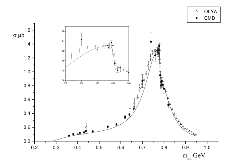
FIG. 7.: $e^{+}e^{-}\rightarrow\pi^{+}\pi^{-}$ cross section. The experimental data are from refs.[31,32].

From definition of function $\alpha_{i}(q^{2})$ in section III we can see this model is unitary only for $q^{2}<4m^{2}$. Thus the effective prediction should be below $m_{\pi\pi}<2m=960$MeV. The result is shown in fig. 7. We can see the prediction agree with data well. Especially, the theoretical prediction in vector meson energy region agree with data excellently. Although the mass parameter $\tilde{m}_{\rho}=803$MeV in $\rho$ propagator is larger than physical mass, the position of pole is localized in $\sqrt{q^{2}}=772$MeV which is just the physical mass of $\rho$. It strongly supports our above discussion and dynamical calculation. It also implies that we must carefully distinguish the physical mass difference of $\rho^{0}$ and $\omega$ from the difference of mass parameter in effective lagrangian.

Let us give some further remarks on pion form factor (8.2). In eq. (8.2), the form factors $\bar{F}_{\gamma\pi\pi}(q^{2})$, $f_{\rho\gamma}(q^{2})$, etc., are all complex function instead of real function. It is caused by one-loop effects of pions. Thus the expression (8.2) can be rewritten as follows:

$$F_{\gamma\pi\pi}(q^{2})=1+q^{2}b_{1}(q^{2})e^{i\phi_{1}(q^{2})}-\frac{q^{4}b_{2}(q^{2})e^{i\phi_{2}(q^{2})}}{2(q^{2}-\tilde{m}_{\rho}^{2}+i\sqrt{q^{2}}\Gamma_{\rho}(q^{2}))}-\frac{q^{4}b_{3}(q^{2})e^{i\phi_{3}(q^{2})}}{6(q^{2}-m_{\omega}^{2}+i\sqrt{q^{2}}\Gamma_{\omega})}.$$ (8.4)

Here $b_{i}(q^{2})(i=1,2,3)$ are three real function and $\phi_{i}(q^{2})(i=1,2,3)$ are three momentum-dependent phases. In particular, $\phi_{3}(q^{2}=m_{\omega}^{2})$, so called Orsay phase, has been extracted from data as $100-125$ degrees[44, 45]. Our theoretical prediction is $\phi_{3}(q^{2}=m_{\omega}^{2})=116.5$ degrees. However, so far, the phases $\phi_{1}(q^{2})$ and $\phi_{2}(q^{2})$ are not reported in any literature. These momentum-dependent phases indicate that the dynamics including loop effects of pseudoscalar mesons is different from one only in tree level. In fig. 8, we given theoretical curves of $\phi_{i}(q^{2})$. They are indeed nontrivial.

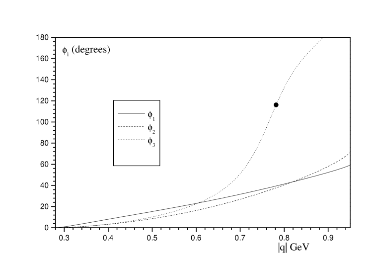
FIG. 8.: $\phi_{i}$ versus $m_{\pi\pi}$ in GeV. Here the solid line denotes the phase shift of non-resonant background $\phi_{1}$, the dash line denotes the phase shift $\phi_{2}$ in $\rho$ coupling and the dot line denotes the phase shift $\phi_{3}$ in $\omega$ coupling. “$\bullet$” denotes Orsay phase.

Obviously, $F_{\pi}(q^{2})$ is an analytic function in the complex $q^{2}$ plane, with a branch cut along the real axis beginning at the two-pion threshold, $q^{2}=4m_{\pi}^{2}$. Time-reversal invariance and the unitarity of the $S$-matrix requires that the phase of the form factor be that of $l=1,\;I=1$ $\pi-\pi$ scattering[47]. This last emerges as $\pi-\pi$ scattering in the relevant channel is very nearly elastic from threshold through $q^{2}\simeq(m_{\pi}+m_{\omega})^{2}$[41, 48]. In this region of $q^{2}$, then, the form factor is related to the $l=1,\;I=1$ $\pi-\pi$ phase shift, $\delta_{1}^{1}$, via[49]

$$F_{\gamma\pi\pi}(q^{2})=e^{2i\delta_{1}^{1}(q^{2})}F_{\gamma\pi\pi}^{*}(q^{2}),$$ (8.5)

so that

$$\tan{\delta_{1}^{1}(q^{2})}=\frac{{\rm Im}F_{\gamma\pi\pi}(q^{2})}{{\rm Re}F_{\gamma\pi\pi}(q^{2})}.$$ (8.6)

The above is a special case of what is sometimes called the Fermi-Watson-Aidzu phase theorem[49, 50]. In fig. 9 and fig. 10 we plot theoretical curves of the $l=1,\;I=1$ $\pi-\pi$ phase shift $\delta_{1}^{1}$ versus $m_{\pi\pi}$ and of $\sin{\delta_{1}^{1}}/p_{\pi}^{3}$ versus $m_{\pi\pi}$ (where $p_{\pi}=\frac{1}{2}\sqrt{q^{2}-4m_{\pi}^{2}}$) respectively. We omit the $\omega$ contribution from our plots of the phase of $F_{\pi}(q^{2})$ for comparing with time-like region pion form factor data [51, 52, 53]. We have also assumed that $\delta_{1}^{1}$ is purely elastic in the regime shown, i.e., the loop effects of $\omega-\pi$ are omitted. The curve predicts $\delta_{1}^{1}\rightarrow 90^{\circ}$ as $\sqrt{q^{2}}\rightarrow 774{\rm MeV}\simeq m_{\rho}$, and $\delta_{1}^{1}>100^{\circ}$ for $\sqrt{q^{2}}>787$MeV. These results agree with data very well.

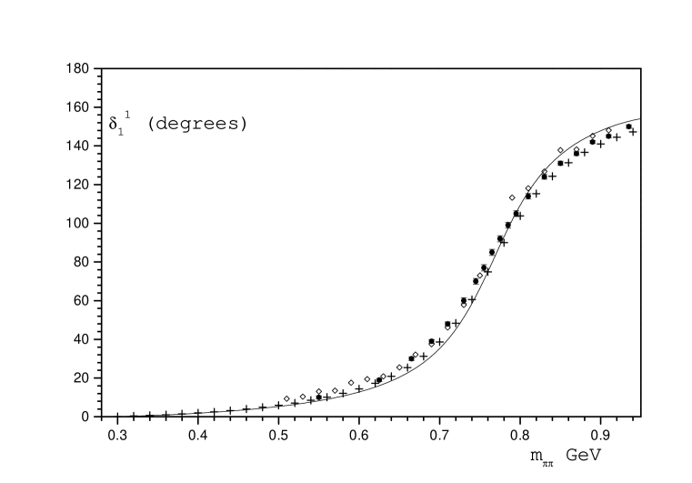
FIG. 9.: The $l=1,\;I=1$ $\pi-\pi$ scattering phase shift. The solid circle point are these from [44], the hollow diamond point are from [45] and “+” denotes the points from [46]. Note that the $\omega$ contribution to the time-like pion form factor phase has been omitted, to facilitate comparison with the empirical phase shift.

Finally we discuss the near threshold behaviour of the form factor. 1) The chiral perturbative theory predicts the form factor at threshold to be $[F_{\gamma\pi\pi}(4m_{\pi}^{2})]_{\rm ChPT}=1.17\pm 0.01$, and ours, $[F_{\pi}(4m_{\pi}^{2})]=1.145$, is close to the ChPT result. 2) The electromagnetic radius of charged pion has been determined to be $\sqrt{<r^{2}>_{\pi}}=0.657\pm 0.027$fm[54], whereas the theoretical prediction in this present paper is $\sqrt{<r^{2}>_{\pi}}=0.645$ fm. 3) The Froggatt-Petersen phase shift function $\sin{\delta_{1}^{1}}/p_{\pi}^{3}$ is connected with the vector-isovector $\pi-\pi$ scattering length $a_{1}^{1}$ through

$$a_{1}^{1}=\lim_{q^{2}\rightarrow 4m_{\pi}^{2}}\frac{\sin{\delta_{1}^{1}}}{p_{\pi}^{3}}.$$ (8.7)

Our theoretical prediction is $a_{1}^{1}=0.037$ in unit of $m_{\pi}^{-3}$. This value is very close to experimental results from $K_{e4}$ data[55, 56] using a Roy equation fit ($a_{1}^{1}=0.038\pm 0.002$) and ChPT prediction $a_{1}^{1}=0.037\pm 0.01$[57] at the two loop order (at $O(p^{4})$).

To provide a brief summary on this section. In section V, it has been revealed that the mass parameter in resonant propagators should be different from its physical mass due to large momentum-dependent width. In this section, this point is confirmed by both of dynamical calculation and phenomenological fit. It also tells us how to understand the mass splitting between $\rho^{0}$ and $\omega$: Although the dynamical calculations show that the mass parameter of $\rho$ in effective lagrangian is even larger than one of $\omega$, the position of pole localized in real axis give their right physical mass splitting. The contribution to this mass splitting from $\rho^{0}-\omega$ mixing is very small, the dominant contribution is from one-loops effects of pseudoscalar mesons. The effective field theory mechanics on $\rho^{0}-\omega$ mass splitting revealed in this present paper is rather subtle. And it is another evident to confirm again that the EMG model is sound.

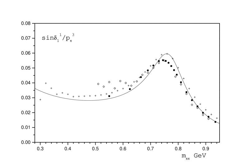
FIG. 10.: Function $\sin{\delta_{1}^{1}}/p_{\pi}^{3}$ deduced from $\pi^{+}\pi^{-}$ phase shift; the function is given in units of $m_{\pi}^{-3}$. The solid circle point are these from [44], the hollow diamond point are from [45] and “+” denotes the points from [46].

IX Light quark masses

The quark masses are some of basic parameters of the standard model. There are various hadronic phenomenology relating to the light quark($u,\;d,\;s$) masses. For instance, they break the chiral symmetry of QCD explicitly. $m_{u}-m_{d}$ breaks isospin symmetry or charge symmetry, and $(m_{u}+m_{d})/2-m_{s}$ breaks SU(3) symmetry in hadron physics respectively. However, in QCD the masses of the light quarks are not directly measurable in inertial experiments, but enter the theory only indirectly as parameters in the fundamental lagrangian. Therefore, it was an active subject to determine light quark masses via phenomenological method.

At low energy, the information about the light quark mass ratios can be extracted in order by order by a rigorous, semiphenomenological method, chiral perturbative theory(ChPT)[4, 6, 58]. To the first order, the results, $m_{s}/m_{d}=19$ and $m_{u}/m_{d}=0.556$, are well-known[59]. Many authors have studied the mass ratios up to next to leading order of the chiral expansion. Gasser and Leutwyler first obtained $m_{s}/m_{d}=20.2$ and $m_{u}/m_{d}=0.554$[4]. Then Kaplan and Manohar extracted $m_{s}/m_{d}=$15 to 23 and $m_{u}/m_{d}=$0 to 0.8 with very larger error bar[60]. These values have been improved to $m_{s}/m_{d}=(20.5\pm 2.5),\;m_{u}/m_{d}=0.52\pm 0.13$ by Leutwyler[61], to $m_{s}/m_{d}=18,\;m_{u}/m_{d}=0.66$ by Gerard[62], and to $m_{s}/m_{d}=21,\;m_{u}/m_{d}=0.30\pm 0.07$ by Donoghue et al.[63] respectively. Finally, Leutwyler analysis previous results and obtained $m_{s}/m_{d}=18.9\pm 0.8,\;m_{u}/m_{d}=0.553\pm 0.043$[64].

Although ChPT provides many information on light quark masses, it is still not enough for further studies on vector meson physics: At chiral limit, the unitarity implies that EMG model can not predict the physics when energy $\sqrt{q^{2}}>2m\simeq 980$MeV. In the other words, to study $\phi(1020)$ physics at chiral limit is not consistent. However, if we take nonzero light quark masses, EMG model will be unitarity when energy $\sqrt{q^{2}}>2(m+m_{s})$. It means that all light flavour vector meson resonances can be included in to EMG model consistently. Hence, the strange quark mass plays important role at $K^{*}$ and $\phi$ physics. Meanwhile, ChPT can only provide information on light quark mass ratio. For obtaining the individual quark masses, other approaches, such as QCD sum rules[65, 66] or lattice calculation[67] are needed. Some authors have pointed out that the determination on the individual quark masses is model-dependent[58]. Thus for studying $K^{*}$ and $\phi$ physics in formalism of EMG model, it is better to determine light quark masses by this model itself.

The Kaplan-Manohar ambiguity of ChPT has caused many debates. In particular, due to this ambiguity, the authors of ref.[68] argued that the observed mass spectrum is consistent with a broad range of quark mass ratios, which specially includes the possibility $m_{u}=0$. However, it is disagreed by other anthors[69, 63]. This problem will also be discussed in EMG model. From lagrangian (2.15), we can see that light current quark masses are defined uniquely in this model, that they are just renormalized “physical” masses of u, d, and s quarks. In principle, therefore, there is no Kaplan-Manohar ambiguity in EMG model. Light current quark masses can be determined uniquely via meson spectrum.

In general, in EMG model the light quark masses can be extracted not only by pseudoscalar meson spectrum, but also by lowest vector meson resonance spectrum. However, one-loop effects of mesons will contribute to vector meson masses. As shown in the above sections, the calculations to every vector meson resonance are very complicate. It makes that the relationship between vector meson spectrum and the light quark masses are also very complicate and indirect. Thus here we will extract information about the light current quark masses from pseudoscalar meson spectrum and their decay constants. The vector meson spectrum will be predicted by this formalism in other paper.

For the purpose of this paper, the lagrangian( 2.15) can be rewritten as follow

$${\cal L}_{\chi}(x)={\cal L}_{q}(x)+{\cal L}_{2}^{(0)}(x)+{\cal L}[\pi(x),\eta_{8}(x)]+{\cal L}[K^{\pm}(x)]+{\cal L}[K^{0}(x)],$$ (9.1)

where ${\cal L}_{q}$ and ${\cal L}_{2}^{(0)}$ are free field lagrangian of constituent quarks of pseudoscalar meson respectively,

$${\cal L}_{q} = \sum_{i=u,d,s}\bar{q}_{i}(i/\!\!\!\partial-\bar{m}_{i})q_{i},\hskip 72.26999pt\bar{m}_{i}=m+m_{i},$$ (9.2)

$${\cal L}_{2}^{(0)} = \frac{F^{2}}{16}<\nabla_{\mu}U\nabla^{\mu}U^{{\dagger}}>$$ (9.3)

$$= \frac{F^{2}}{8}{\partial_{\mu}\Phi^{a}\partial^{\mu}\Phi^{a}+4a_{\mu}^{a}\partial^{\mu}\Phi^{a}+\cdots},\hskip 36.135pta=1,2,\cdots,8.$$ (9.4)

${\cal L}[\Phi(x)]$ denotes quark-meson coupling lagrangian,

$${\cal L}[\pi,\eta_{8}] = \frac{g_{A}}{\sqrt{2}}[(\partial_{\mu}\pi^{+}+2a_{\mu}^{+})\bar{u}\gamma^{\mu}\gamma_{5}d+c.c.]+\frac{g_{A}}{2}\sum_{i=u,d,s}(\partial_{\mu}P_{i}+2A_{\mu}^{(i)})\bar{q}_{i}\gamma^{\mu}\gamma_{5}q_{i}$$ (9.7)

$$+\frac{i}{\sqrt{2}}\kappa(m_{u}+m_{d})(\pi^{+}\bar{u}\gamma_{5}d+c.c.)+i\kappa\sum_{i=u,d,s}m_{i}P_{i}\bar{q}_{i}\gamma_{5}q_{i}$$

$$+\frac{1}{2}(m_{u}+m_{d})\pi^{+}\pi^{-}(\bar{u}u+\bar{d}d)+\frac{1}{2}\sum_{i=u,d,s}m_{i}P_{i}^{2}\bar{q}_{i}q_{i},$$

$${\cal L}[K^{\pm}] = \frac{g_{A}}{\sqrt{2}}[(\partial_{\mu}K^{+}+2A_{\mu}^{+})\bar{u}\gamma^{\mu}\gamma_{5}s+c.c.]+\frac{i}{\sqrt{2}}\kappa(m_{u}+m_{s})(K^{+}\bar{u}\gamma_{5}s+c.c.)$$ (9.9)

$$+\frac{1}{2}(m_{u}+m_{s})K^{+}K^{-}(\bar{u}u+\bar{s}s),$$

$${\cal L}[K^{0}] = \frac{g_{A}}{\sqrt{2}}[(\partial_{\mu}K^{0}+2A_{\mu}^{0})\bar{d}\gamma^{\mu}\gamma_{5}s+(\partial_{\mu}\bar{K}^{0}+2\bar{A}_{\mu}^{0})d\gamma^{\mu}\gamma_{5}\bar{s}]$$ (9.11)

$$+\frac{i}{\sqrt{2}}\kappa(m_{d}+m_{s})(K^{0}\bar{d}\gamma_{5}s+\bar{K}^{0}d\gamma_{5}\bar{s})+\frac{1}{2}(m_{d}+m_{s})K^{0}\bar{K}^{0}(\bar{d}d+\bar{s}s),$$

where $c.c.$ denotes charge conjugate term of previous term,

$$P_{u}=\pi_{3}+\frac{1}{\sqrt{3}}\eta_{8},\;\;\;\;\;\;\;\;P_{d}=-\pi_{3}+\frac{1}{\sqrt{3}}\eta_{8},\;\;\;\;\;\;\;\;P_{s}=-\frac{2}{\sqrt{3}}\eta_{8},$$ (9.12)

and $a_{\mu}^{a}$, $A_{\mu}^{(u)},\;A_{\mu}^{(d)}$ and $A_{\mu}^{(s)}$ etc. are axial-vector external fields corresponding these pseudoscalar meson fields. From eq. (9.7) we can see that the $K^{\pm}$-quark coupling and $K^{0}$-quark coupling are similar to $\pi^{\pm}$-quark coupling. Thus we only need to calculate masses and decay constants of $\pi^{\pm},\;\pi^{0}$ and $\eta^{8}$. Then masses and decay constants of $K^{\pm}$ can be obtained via replacing $m_{d}$ by $m_{s}$ in one of $\pi^{\pm}$, and masses and decay constants of $K^{0}$ can be obtained via replacing $m_{u}$ by $m_{s}$ in one of $\pi^{\pm}$.

At large $N_{c}$ limit, the kinetic terms of pseudoscalar mesons can be obtained via calculating one-point and two-point effective action. Note that here the light quark masses will not be expanded perturbatively, but enter quark propagator and be evaluated in non-perturbative method. Explicitly, the kinetic term of charge pion fields reads

$${\cal L}_{2}[\pi^{\pm}(x)] = \frac{F^{2}(m_{u},m_{d})}{4}\partial_{\mu}\pi^{+}\partial^{\mu}\pi^{-}+\frac{\bar{f}^{2}(m_{u},m_{d})}{2}(a_{\mu}^{+}\partial^{\mu}\pi^{-}+c.c.)-\frac{F_{0}^{2}}{4}\bar{M}^{2}(m_{u},m_{d})\pi^{+}\pi^{-}$$ (9.14)

$$+\int\frac{d^{4}q}{(2\pi)^{4}}e^{iq\cdot x}\{\frac{\alpha(q^{2};m_{u},m_{d})}{2}iq^{\mu}(a_{\mu}^{+}(x)\pi^{-}(q)+c.c.)-\frac{F_{0}^{2}}{4}\beta(q^{2};m_{u},m_{d}))\pi^{+}(q)\pi^{-}(x)\},$$

where

$$F^{2}(m_{u},m_{d})=F_{0}^{2}+\frac{3}{2}g^{2}g_{A}^{2}m_{ud}(2m+\bar{m}_{ud})+3g^{2}\kappa g_{A}m_{ud}\bar{m}_{ud}$$ (9.15)

$$\;\;\;\;\;\;\;\;-\frac{N_{c}}{2\pi^{2}}g_{A}(g_{A}\bar{m}_{ud}+2\kappa m_{ud})\int_{0}^{1}dt[\bar{m}_{u}+t(m_{d}-m_{u})]\ln{(x_{u}^{2}+t(x_{d}^{2}-x_{u}^{2}))}$$ (9.16)

$$\;\;\;\;\;\;\;\;+4\kappa^{2}m_{ud}^{2}\{(\frac{g^{2}}{4}-\frac{F_{0}^{2}B_{0}}{48m^{3}}-\frac{N_{c}}{24\pi^{2}})-\frac{N_{c}}{8\pi^{2}}\int_{0}^{1}dt\cdot t(1-t)[3\ln{(x_{u}^{2}+t(x_{d}^{2}-x_{u}^{2}))}-\frac{\bar{m}_{u}\bar{m}_{d}}{\bar{m}_{u}^{2}+t(\bar{m}_{d}^{2}-\bar{m}_{u}^{2})}]\},$$ (9.17)

$$\bar{f}^{2}(m_{u},m_{d})=F_{0}^{2}+\frac{3}{2}g^{2}g_{A}^{2}m_{ud}(4m+\bar{m}_{ud})+\frac{3}{2}g^{2}\kappa g_{A}m_{ud}\bar{m}_{ud}$$ (9.18)

$$\;\;\;\;\;\;\;\;-\frac{N_{c}}{2\pi^{2}}g_{A}(g_{A}\bar{m}_{ud}+\kappa m_{ud}+m_{d})\int_{0}^{1}dt[\bar{m}_{u}+t(m_{d}-m_{u})]\ln{(x_{u}^{2}+t(x_{d}^{2}-x_{u}^{2}))},$$ (9.19)

$$\bar{M}^{2}(m_{u},m_{d})=B_{0}m_{ud}\{\frac{1}{2}(x_{u}^{3}+x_{d}^{3})+\frac{N_{c}}{2\pi^{2}}\frac{m^{3}}{F_{0}^{2}B_{0}}(x_{u}^{3}\ln{x_{u}^{2}}+x_{d}^{3}\ln{x_{d}^{3}})-\frac{\kappa^{2}}{4}\frac{m_{ud}}{m}(x_{u}^{2}+x_{d}^{2})\}$$ (9.20)

$$\;\;\;\;\;\;\;\;+\frac{3}{2}g^{2}\kappa^{2}\frac{(m_{d}^{2}-m_{u}^{2})^{2}}{F_{0}^{2}}-\frac{N_{c}}{2\pi^{2}}\kappa^{2}\frac{m_{ud}^{2}}{F_{0}^{2}}\int_{0}^{1}dt[2\bar{m}_{u}^{2}-\bar{m}_{u}\bar{m}_{d}+2t(\bar{m}_{d}^{2}-\bar{m}_{u}^{2})]\ln{(x_{u}^{2}+t(x_{d}^{2}-x_{u}^{2}))},$$ (9.21)

$$\alpha(q^{2};m_{u},m_{d})=-\frac{N_{c}}{2\pi^{2}}g_{A}(g_{A}\bar{m}_{ud}+\kappa m_{ud})\int_{0}^{1}dt[\bar{m}_{u}+t(m_{d}-m_{u})]\ln{\left(1-\frac{t(1-t)q^{2}}{\bar{m}_{u}^{2}+t(\bar{m}_{d}^{2}-\bar{m}_{u}^{2})}\right)},$$ (9.22)

$$\beta(q^{2};m_{u},m_{d})=\frac{N_{c}}{2\pi^{2}}g_{A}\frac{q^{2}}{F_{0}^{2}}(g_{A}\bar{m}_{ud}+2\kappa m_{ud})\int_{0}^{1}dt[\bar{m}_{u}+t(m_{d}-m_{u})]\ln{\left(1-\frac{t(1-t)q^{2}}{\bar{m}_{u}^{2}+t(\bar{m}_{d}^{2}-\bar{m}_{u}^{2})}\right)}$$ (9.23)

$$\;\;\;\;\;\;\;\;-\frac{N_{c}}{2\pi^{2}}\kappa^{2}\frac{m_{ud}^{2}}{F_{0}^{2}}\int_{0}^{1}dt\{[2\bar{m}_{u}^{2}-\bar{m}_{u}\bar{m}_{d}+2t(\bar{m}_{d}^{2}-\bar{m}_{u}^{2})-3t(1-t)q^{2}]\ln{\left(1-\frac{t(1-t)q^{2}}{\bar{m}_{u}^{2}+t(\bar{m}_{d}^{2}-\bar{m}_{u}^{2})}\right)}$$ (9.24)

$$\hskip 144.54pt+t(1-t)q^{2}\left(2-\frac{\bar{m}_{u}\bar{m}_{d}}{\bar{m}_{u}^{2}+t(\bar{m}_{d}^{2}-\bar{m}_{u}^{2})}\right)\},$$ (9.25)

where $m_{ij}=m_{i}+m_{j}$ and $\bar{m}_{ij}=\bar{m}_{i}+\bar{m}_{j}(i,j=u,d,s)$. It should be pointed out that $\alpha(q^{2};m_{u},m_{d})$ is order $q^{2}$ at least and $\beta(q^{2};m_{u},m_{d})$ is order $q^{4}$ at least. Since in this paper we focus on pseudoscalar meson spectrum, these high order derivative terms should obey motion equation of pseudoscalar mesons. In momentum space, the motion equation of physical pseudoscalar mesons is generally written

$$(q^{2}-m_{\varphi}^{2})\varphi(q)=-if_{\varphi}q^{\mu}A_{\mu}^{(\varphi)}(-q),$$ (9.26)

where $m_{\varphi}$ and $f_{\varphi}$ are physical mass and decay constants of pseudoscalar, e.g., $m_{\pi}=135$MeV and $f_{\pi}=185.2$MeV. Due to this motion equation, we have

$$\alpha(q^{2};m_{u},m_{d})a_{\mu}^{+}(x)\pi^{-}(q) = \alpha(m_{\pi}^{2};m_{u},m_{d})a_{\mu}^{+}(x)\pi^{-}(q),$$ (9.27)

$$\beta(q^{2};m_{u},m_{d})\pi^{+}(q)\pi^{-}(-q) = \beta(m_{\pi}^{2};m_{u},m_{d})\pi^{+}(q)\pi^{-}(-q)-\frac{i}{2}q^{\mu}f_{\pi}\beta^{\prime}(m_{\pi}^{2};m_{u},m_{d})(a_{\mu}^{+}(x)\pi^{-}(q)+c.c.),$$ (9.28)

where

$$\beta^{\prime}(m_{\pi}^{2};m_{u},m_{d})=\frac{d}{dq^{2}}\beta^{\prime}(q^{2};m_{u},m_{d})|_{q^{2}=m_{\pi}^{2}}.$$ (9.29)

Thus eq.( 3.15) can be rewritten

$${\cal L}_{2}[\pi^{\pm}(x)] = \frac{F^{2}(m_{u},m_{d})}{4}\partial_{\mu}\pi^{+}\partial^{\mu}\pi^{-}-\frac{F_{0}^{2}}{4}\{\bar{M}^{2}(m_{u},m_{d})+\beta(m_{\pi}^{2};m_{u},m_{d})\}\pi^{+}\pi^{-}$$ (9.31)

$$+\{\frac{\bar{f}^{2}(m_{u},m_{d})}{2}+\frac{\alpha(m_{\pi}^{2};m_{u},m_{d})}{2}+\frac{F_{0}^{2}}{4F(m_{u},m_{d})}f_{\pi}\beta^{\prime}(m_{\pi}^{2};m_{u},m_{d})\}(a_{\mu}^{+}\partial^{\mu}\pi^{-}+c.c.).$$

The kinetic term of $\pi^{0}$ and $\eta_{8}$ reads

$${\cal L}_{2}[\pi^{0}(x),\eta_{8}(x)]=\sum_{i=u,d,s}\{\frac{F_{i}^{2}(m_{i})}{8}\partial_{\mu}P_{i}\partial^{\mu}P_{i}-\frac{F_{0}^{2}}{8}\bar{M}_{i}^{2}(m_{i})P_{i}^{2}-\frac{F_{0}^{2}}{8}\int\frac{d^{4}q}{(2\pi)^{4}}e^{iq\cdot x}\beta_{i}(q^{2};m_{i})P_{i}(q)P_{i}(x)\},$$ (9.32)

where

$$F_{i}^{2}(m_{i}) = \frac{F_{0}^{2}}{2}+3g^{2}g_{A}^{2}m_{i}(2m+m_{i})+6g^{2}\kappa g_{A}m_{i}\bar{m}_{i}+8\kappa^{2}(\frac{g^{2}}{4}-\frac{F_{0}^{2}B_{0}}{48m^{3}}-\frac{N_{c}}{48\pi^{2}})m_{i}^{2}$$ (9.34)

$$-\frac{N_{c}}{2\pi^{2}}(g_{A}^{2}\bar{m}_{i}^{2}+2g_{A}\kappa m_{i}\bar{m}_{i}+\kappa^{2}m_{i}^{2})\ln{x_{i}^{2}},$$

$$\bar{M}_{i}^{2}(m_{i}) = (B_{0}+\frac{N_{c}}{\pi^{2}}\frac{m^{3}}{F_{0}^{2}}\ln{x_{i}^{2}})m_{i}x_{i}^{2}(x_{i}-\frac{m_{i}}{m}\kappa^{2}),$$ (9.35)

$$\beta_{i}(q^{2};m_{i}) = \frac{N_{c}}{2\pi^{2}F_{0}^{2}}q^{2}\{\frac{\kappa^{2}}{3}m_{i}^{2}+\left(g_{A}^{2}\bar{m}_{i}^{2}+2\kappa m_{i}\bar{m}_{i}+2\kappa^{2}m_{i}^{2}[\bar{m}_{i}^{2}q^{-2}-3t(1-t)]\right)\int_{0}^{1}dt\ln{(1-\frac{t(1-t)q^{2}}{\bar{m}_{i}^{2}})}\}.$$ (9.36)

Since the decay constants for neutral mesons cannot be extracted directly from the data. It means that the decay constants for neutral mesons can not be used to determine light current quark masses. Therefore, in this paper we do not need to evaluate the decay constants for neutral pion and $\eta_{8}$. In addition, because auxiliary fields $P_{i}$ do not lie in physical hadron spectrum, the equation of motion (9.26) can not be used in (9.32) simply. We will use propagator method to deal with the terms with high power momenta in (9.32) and diagonalize $\pi_{3}-\eta_{8}$ mixing.

Next we evaluate one-loop effects of pseudoscalar mesons. Due to parity conservation, there are only tadpole diagrams of pseudoscalar mesons contributing to masses of decay constants of $0^{-}$ mesons(fig. 1). Moreover, we can expect that, in mass spectrum and decay constants of pseudoscalar mesons, the dominant one-loop effects is generated by the lowest order effective lagrangian, because neglect is $O(m_{q}^{3})$ and suppressed by $N_{c}^{-1}$ expansion. It is fortunate that the formalism is renormalized up to this order.

The lowest order effective lagrangian is well-known

$${\cal L}_{2} = \frac{F_{0}^{2}}{16}<\nabla_{\mu}U\nabla^{\mu}U^{{\dagger}}+\chi U^{{\dagger}}+U\chi^{{\dagger}}>$$ (9.37)

$$= \frac{F_{0}^{2}}{48}<[\lambda^{a},\Delta_{\mu}][\lambda^{a},\Delta^{\mu}]>+\frac{3F_{0}^{2}}{256}<\lambda^{a}\lambda^{a}(\xi\chi^{{\dagger}}\xi+\xi^{{\dagger}}\chi\xi^{{\dagger}})>,$$ (9.38)

Substituting expansion( 4.1) into ${\cal L}_{2}$ and retaining terms up to and including $\varphi^{2}$ one obtains

$${\cal L}_{2}\rightarrow\bar{\cal L}_{2}+\frac{F_{0}^{2}}{8}(\partial_{\mu}\varphi^{a}\partial^{\mu}\varphi^{a}-m_{\varphi}^{2}\varphi^{a}\varphi^{a})-\frac{F_{0}^{2}}{16}<[\varphi,\Delta_{\mu}][\varphi,\Delta^{\mu}]+\frac{1}{4}\{\varphi,\varphi\}(\bar{\xi}\chi^{{\dagger}}\bar{\xi}+\bar{\xi}^{{\dagger}}\chi\bar{\xi}^{{\dagger}}-2{\cal M})>,$$ (9.39)

where we have omitted some terms which do not contribute to masses and decay constants via one-loop graphs. The contribution of tadpole graphs can be calculated easily

$${\cal L}_{2}^{(\rm tad)} = -\frac{1}{4}<[\lambda^{a},\Delta_{\mu}][\lambda^{a},\Delta^{\mu}]+\frac{1}{4}\{\lambda^{a},\lambda^{a}\}(\bar{\xi}\chi^{{\dagger}}\bar{\xi}+\bar{\xi}^{{\dagger}}\chi\bar{\xi}^{{\dagger}}-2{\cal M})>\int\frac{d^{4}k}{(2\pi)^{4}}\frac{i}{k^{2}-m_{\varphi}^{2}+i\epsilon}$$ (9.40)

$$= \frac{1}{4}(m_{\varphi}^{2}N_{\epsilon}-\frac{m_{\varphi}^{2}}{16\pi^{2}}\ln{\frac{m_{\varphi}^{2}}{\mu^{2}}})<[\lambda^{a},\Delta_{\mu}][\lambda^{a},\Delta^{\mu}]+\frac{1}{4}\{\lambda^{a},\lambda^{a}\}(\bar{\xi}\chi^{{\dagger}}\bar{\xi}+\bar{\xi}^{{\dagger}}\chi\bar{\xi}^{{\dagger}}-2{\cal M})>,$$ (9.41)

where

$$N_{\epsilon}=\frac{1}{16\pi^{2}}\{\frac{2}{\epsilon}+\ln{(4\pi)}+\gamma+1\}.$$

Comparing eq.( 9.40) and eq.( 9.34) we can see that the divergence $N_{\epsilon}$ can be absorbed by free parameters $F_{0}$ and $B_{0}$. Thus the sum of tree graphs and tadpole contribution is

$${\cal L}_{2}^{(t)}=\frac{F_{0}^{2}}{48}(1-3\mu_{\varphi})v<[\lambda^{a},\Delta_{\mu}][\lambda^{a},\Delta^{\mu}]>+\frac{3F_{0}^{2}}{256}(1-\frac{8}{3}\mu_{\varphi})<\lambda^{a}\lambda^{a}(\xi\chi^{{\dagger}}\xi+\xi^{{\dagger}}\chi\xi^{{\dagger}})>,$$ (9.42)

where

$$\mu_{\varphi}=\frac{m_{\varphi}^{2}}{4\pi^{2}F_{0}^{2}}\ln{\frac{m_{\varphi}^{2}}{\mu^{2}}}.$$ (9.43)

Here we appoint that $m_{\varphi}=m_{\pi}$ when $a=1,2,3$, $m_{\varphi}=m_{{}_{K}}$ when $a=4,5,6,7$ and $m_{\varphi}=m_{\eta_{8}}$ when $a=8$.

For extracting $(m_{{}_{K^{+}}})_{\rm QCD}$ from experimental data, the electromagnetic mass splitting of $K$-meson is required. The prediction of Dashen theorem[70], $(m_{{}_{K^{+}}}-m_{{}_{K^{0}}})_{e.m.}=1.3$MeV, has been corrected in several recent analysis with considering contribution from vector meson exchange. A larger correction is first obtained by Donoghue, Holstein and Wyler[71], who find $(m_{{}_{K^{+}}}-m_{{}_{K^{0}}})_{e.m.}=2.3$MeV. Then Bijnens and Prades[72], who evaluated both long-distance contribution using ENJL model and short-distance contribution using perturbative QCD and factorization, find $(m_{{}_{K^{+}}}-m_{{}_{K^{0}}})_{e.m.}=2.4\pm 0.3$MeV at $\mu=m_{\rho}$. Gao et.al.[73] also gave $(m_{{}_{K^{+}}}-m_{{}_{K^{0}}})_{e.m.}=2.5$MeV. Baur and Urech[74], however, obtained a smaller correction, $(m_{{}_{K^{+}}}-m_{{}_{K^{0}}})_{e.m.}=1.6$MeV at $\mu=m_{\rho}$. In addition, calculation of lattice QCD[75] found $(m_{{}_{K^{+}}}-m_{{}_{K^{0}}})_{e.m.}=1.9$MeV. These estimates indicate that the corrections to Dashen theorem are indeed substantial. In this the present paper, we average the above results and take $(m_{{}_{K^{+}}}-m_{{}_{K^{0}}})_{e.m.}=2.1\pm 0.1$MeV at energy scale $\mu=m_{\rho}$.

From eqs. (9.31) and (9.42), the masses and decay constants of koan and charge pion can be obtained via solve the following equations

$$m_{\pi^{+}}^{2} = \frac{F_{0}^{2}}{F_{{}_{R}}^{2}(m_{u},m_{d})}\{\bar{M}_{{}_{R}}^{2}(m_{u},m_{d})+\beta(m_{\pi}^{2};m_{u},m_{d})\}$$ (9.44)

$$m_{{}_{K^{+}}}^{2} = \frac{F_{0}^{2}}{F_{{}_{R}}^{2}(m_{u},m_{s})}\{\bar{M}_{{}_{R}}^{2}(m_{u},m_{s})+\beta(m_{{}_{K}}^{2};m_{u},m_{s})\},$$ (9.45)

$$m_{{}_{K^{0}}}^{2} = \frac{F_{0}^{2}}{F_{{}_{R}}^{2}(m_{d},m_{s})}\{\bar{M}_{{}_{R}}^{2}(m_{d},m_{s})+\beta(m_{{}_{K}}^{2};m_{d},m_{s})\},$$ (9.46)

$$f_{\pi^{+}} = \frac{\bar{f}_{{}_{R}}^{2}(m_{u},m_{d})}{F_{{}_{R}}(m_{u},m_{d})}+\frac{\alpha(m_{\pi}^{2};m_{u},m_{d})}{F_{{}_{R}}(m_{u},m_{d})}+\frac{F_{0}^{2}}{2F_{{}_{R}}^{2}(m_{u},m_{d})}f_{\pi^{+}}\beta^{\prime}(m_{\pi}^{2};m_{u},m_{d}),$$ (9.47)

$$f_{{}_{K^{+}}} = \frac{\bar{f}_{{}_{R}}^{2}(m_{u},m_{s})}{F_{{}_{R}}(m_{u},m_{s})}+\frac{\alpha(m_{{}_{K}}^{2};m_{u},m_{s})}{F_{{}_{R}}(m_{u},m_{s})}+\frac{F_{0}^{2}}{2F_{{}_{R}}^{2}(m_{u},m_{s})}f_{{}_{K}}\beta^{\prime}(m_{{}_{K}}^{2};m_{u},m_{s}),$$ (9.48)

$$f_{{}_{K^{0}}} = \frac{\bar{f}_{{}_{R}}^{2}(m_{d},m_{s})}{F_{{}_{R}}(m_{d},m_{s})}+\frac{\alpha(m_{{}_{K}}^{2};m_{d},m_{s})}{F_{{}_{R}}(m_{d},m_{s})}+\frac{F_{0}^{2}}{2F_{{}_{R}}^{2}(m_{d},m_{s})}f_{{}_{K}}\beta^{\prime}(m_{{}_{K}}^{2};m_{d},m_{s}),$$ (9.49)

where subscript “R” denotes renormalized quantity,

$$F_{{}_{R}}^{2}(m_{u},m_{d}) = F^{2}(m_{u},m_{d})-F_{0}^{2}(2\mu_{\pi}+\mu_{{}_{K}}),$$ (9.50)

$$F_{{}_{R}}^{2}(m_{i},m_{s}) = F^{2}(m_{i},m_{s})-\frac{3}{4}F_{0}^{2}(\mu_{\pi}+2\mu_{{}_{K}}+\mu_{\eta_{8}}),\hskip 72.26999pt(i=u,d)$$ (9.51)

$$\bar{M}_{{}_{R}}^{2}(m_{u},m_{d}) = \bar{M}^{2}(m_{u},m_{d})-B_{0}(m_{u}+m_{d})(\frac{3}{2}\mu_{\pi}+\mu_{{}_{K}}+\frac{1}{6}\mu_{\eta_{8}}),$$ (9.52)

$$\bar{M}_{{}_{R}}^{2}(m_{i},m_{s}) = \bar{M}^{2}(m_{i},m_{s})-B_{0}(m_{i}+m_{s})(\frac{3}{4}\mu_{\pi}+\frac{3}{2}\mu_{{}_{K}}+\frac{5}{12}\mu_{\eta_{8}}),$$ (9.53)

$$\bar{f}_{{}_{R}}^{2}(m_{u},m_{d}) = \bar{f}^{2}(m_{u},m_{d})-F_{0}^{2}(2\mu_{\pi}+\mu_{{}_{K}}),$$ (9.54)

$$\bar{f}_{{}_{R}}^{2}(m_{i},m_{s}) = \bar{f}^{2}(m_{i},m_{s})-\frac{3}{4}F_{0}^{2}(\mu_{\pi}+2\mu_{{}_{K}}+\mu_{\eta_{8}}),$$ (9.55)

Here the quantity $\mu_{\varphi}$ depends on the renormalization scale $\mu$. It has been recognized that the scale plays an important role in low-energy QCD. In this formalism, many parameters, such as light current quark masses, constituent quark mass $m$, axial-vector coupling constant $g_{A}$, are scale-dependent. The characteristic scale of the model is described by the universal coupling constant $g$ which is determined by the first KSRF sum rule at energy scale $\mu=m_{\rho}$. Hence we take $\mu=m_{\rho}=770$MeV in $\mu_{\varphi}$, and the physical masses and decay constants, however, should be independent of the renormalization scale.

In order to obtain the masses of $\pi^{0}$ and $\eta^{8}$, the $\pi_{3}-\eta_{8}$ mixing in eq. (9.32) must be diagonalized. Eq.(9.32) together with eq.(9.42) lead to the quadratic terms for the $\pi_{3}$ and $\eta_{8}$ are of the form

$$S_{2}[\pi_{3},\eta_{8}]=\int\frac{d^{4}q}{(2\pi)^{4}}\{\frac{1}{2}(q^{2}-M_{3}^{2}(q^{2}))\pi_{3}^{2}+\frac{1}{2}(q^{2}-M_{8}^{2}(q^{2}))\eta_{8}^{2}-M_{38}^{2}(q^{2})\pi_{3}\eta_{8}\}$$ (9.56)

where

$$M_{3}^{2}(q^{2}) = \frac{F_{0}^{2}}{F_{3}^{2}}\{\bar{M}_{u}^{2}(m_{u})+\bar{M}_{d}^{2}(m_{d})+\beta_{u}(q^{2};m_{u})+\beta_{d}(q^{2};m_{d})-2B_{0}\hat{m}(\frac{3}{2}\mu_{\pi}+\mu_{{}_{K}}+\frac{1}{6}\mu_{\eta_{8}})\},$$ (9.57)

$$M_{8}^{2}(q^{2}) = \frac{F_{0}^{2}}{3F_{8}^{2}}\{\bar{M}_{u}^{2}(m_{u})+\bar{M}_{d}^{2}(m_{d})+4\bar{M}_{s}^{2}(m_{s})+\beta_{u}(q^{2};m_{u})+\beta_{d}(q^{2};m_{d})+4\beta_{s}(q^{2};m_{s})$$ (9.59)

$$-2B_{0}(\hat{m}+2m_{s})(2\mu_{{}_{K}}+\frac{2}{3}\mu_{\eta_{8}})-2B_{0}\hat{m}(-\frac{3}{2}\mu_{\pi}+\mu_{{}_{K}}+\frac{1}{2}\mu_{\eta_{8}})\},$$

$$M_{38}^{2}(q^{2}) = \frac{F_{0}^{2}}{\sqrt{3}F_{3}F_{8}}\{\bar{M}_{u}^{2}(m_{u})-\bar{M}_{d}^{2}(m_{d})+\beta_{u}(q^{2};m_{u})-\beta_{d}(q^{2};m_{d})-B_{0}(m_{u}-m_{d})(\frac{3}{2}\mu_{\pi}+\mu_{{}_{K}}+\frac{1}{6}\mu_{\eta_{8}})\}$$ (9.61)

$$+q^{2}\frac{F_{u}^{2}(m_{u})-F_{d}^{2}(m_{d})}{\sqrt{3}F_{3}F_{8}},$$

with $\hat{m}=(m_{u}+m_{d})/2$ and

$$F_{3}^{2} = F_{u}^{2}(m_{u})+F_{d}^{2}(m_{d})-F_{0}^{2}(2\mu_{\pi}+\mu_{{}_{K}}),$$ (9.62)

$$F_{8}^{2} = \frac{1}{3}\{F_{u}^{2}(m_{u})+F_{d}^{2}(m_{d})+4F_{s}^{2}(m_{s})\}-3F_{0}^{2}\mu_{{}_{K}}.$$ (9.63)

Due to $\pi_{3}-\eta_{8}$ mixing, the “physical” propagators of $\pi^{0}$ and $\eta_{8}$ are obtained via the chain approximation in momentum space

$$\frac{i}{q^{2}-m_{\pi^{0}}^{2}+i\epsilon} = \frac{i}{q^{2}-M_{3}^{2}(q^{2})+i\epsilon}+\frac{iM_{38}^{4}(q^{2})}{(q^{2}-M_{8}^{2}(q^{2})+i\epsilon)(q^{2}-M_{3}^{2}(q^{2})+i\epsilon)^{2}}+\cdots$$ (9.64)

$$= \frac{i}{q^{2}-M_{3}^{2}(q^{2})-\frac{M_{38}^{4}(q^{2})}{q^{2}-M_{8}^{2}(q^{2})}+i\epsilon},$$ (9.65)

$$\frac{i}{q^{2}-m_{\eta_{8}}^{2}+i\epsilon} = \frac{i}{q^{2}-M_{8}^{2}(q^{2})+i\epsilon}+\frac{iM_{38}^{4}(q^{2})}{(q^{2}-M_{3}^{2}(q^{2})+i\epsilon)(q^{2}-M_{8}^{2}(q^{2})+i\epsilon)^{2}}+\cdots$$ (9.66)

$$= \frac{i}{q^{2}-M_{8}^{2}(q^{2})-\frac{M_{38}^{4}(q^{2})}{q^{2}-M_{3}^{2}(q^{2})}+i\epsilon}.$$ (9.67)

Then the masses of $\pi^{0}$ and $\eta_{8}$ are just solutions of the following equations,

$$m_{\pi^{0}}^{2} = M_{3}^{2}(m_{\pi^{0}}^{2})+\frac{M_{38}^{2}(m_{\pi^{0}}^{2})}{m_{\pi^{0}}^{2}-M_{8}^{2}(m_{\pi^{0}}^{2})},$$ (9.68)

$$m_{\eta^{8}}^{2} = M_{8}^{2}(m_{\eta_{8}}^{2})+\frac{M_{38}^{2}(m_{\eta_{8}}^{2})}{m_{\eta_{8}}^{2}-M_{8}^{2}(m_{\eta_{8}}^{2})}.$$ (9.69)

In the above results, the parameters $\kappa$, $F_{0}$ and $B_{0}$ are still not determined. In order to determine them and three light quark masses, six inputs are required. In this paper we choose $f_{\pi^{+}}=185.2\pm 0.5$MeV, $f_{{}_{K^{+}}}=226.0\pm 2.5$MeV, $m_{\pi^{0}}=134.98$MeV, $m_{{}_{K^{0}}}=497.67$MeV and $(m_{{}_{K^{+}}})_{\rm QCD}=491.6\pm 0.1$MeV. Another input is $m_{d}-m_{u}=3.9\pm 0.22$MeV, which is extracted from $\omega\rightarrow\pi^{+}\pi^{-}$ decay at energy scale $\mu=m_{\rho}$. Recalling $m=480$MeV, $g_{A}=0.75$ and $g=\pi^{-1}$ for $N_{c}=3$, we can fit light quark masses as in table 1.

In table 1, the errors of results are from uncertainties in decay constant of $K^{+}$. electromagnetic mass splitting of $K$-mesons and isospin violation parameter $m_{d}-m_{u}$ respectively. The first column in table 1 we show the results for $f_{{}_{K^{+}}}=223.5$MeV. The third column corresponds the center value of $f_{{}_{K^{+}}}$, $226.0$MeV and the fifth column corresponds $f_{{}_{K^{+}}}=228.5$MeV. Then from table 1 we have

$$m_{s} = 160\pm 15.5{\rm MeV},\hskip 36.135ptm_{d}=7.9\pm 2.7{\rm MeV},\hskip 36.135ptm_{u}=4.1\pm 1.5{\rm MeV},$$ (9.70)

$$\frac{m_{s}}{m_{d}} = 20.2\pm 3.0,\hskip 57.81621pt\frac{m_{u}}{m_{d}}=0.5\pm 0.09.$$ (9.71)

Here the large errors are from the uncertainty of $f_{{}_{K^{+}}}$. We can see that our results agree with one obtained by other various approaches(e.g., QCD sum rule or ChPT) well. From table 1 we also have $(m_{\pi^{+}}-m_{\pi^{0}})_{\rm QCD}=-0.25$MeV (where the contribution from $\pi_{3}-\eta^{\prime}$ mixing is neglected). This result allows that the electromagnetic mass splitting of pion is $(m_{\pi^{+}}-m_{\pi^{0}})_{\rm e.m.}=4.8$MeV.

Finally, it is interesting to expand non-perturtation results (5.1) up to the next to leading order of the chiral expansion and compare with one of ChPT. If we neglect the mass difference $m_{d}-m_{u}$, up to this order the masses of decay constants of koan and pion read

$$m_{\pi}^{2} = B_{0}(m_{u}+m_{d})\{1+\frac{1}{2}\mu_{\pi}-\frac{1}{6}\mu_{\eta_{8}}+[\frac{1}{2}(3-\kappa^{2})+\frac{3m^{2}}{\pi^{2}F_{0}^{2}}(\frac{m}{B_{0}}-\kappa g_{A}-\frac{g_{A}^{2}}{2}-\frac{B_{0}}{6m}g_{A}^{2})]\frac{m_{u}+m_{d}}{m}\},$$ (9.72)

$$m_{{}_{K}}^{2} = B_{0}(\hat{m}+m_{s})\{1+\frac{1}{3}\mu_{\eta_{8}}+[\frac{1}{2}(3-\kappa^{2})+\frac{3m^{2}}{\pi^{2}F_{0}^{2}}(\frac{m}{B_{0}}-\kappa g_{A}-\frac{g_{A}^{2}}{2}-\frac{B_{0}}{6m}g_{A}^{2})]\frac{\hat{m}+m_{s}}{m}\},$$ (9.73)

$$f_{\pi} = F_{0}\{1-\mu_{\pi}-\frac{1}{2}\mu_{{}_{K}}+\frac{3}{2\pi^{2}}g_{A}^{2}\frac{m(m_{u}+m_{d})}{F_{0}^{2}}\},$$ (9.74)

$$f_{{}_{K}} = F_{0}\{1-\frac{3}{8}\mu_{\pi}-\frac{3}{4}\mu_{{}_{K}}-\frac{3}{8}\mu_{\eta_{8}}+\frac{3}{2\pi^{2}}g_{A}^{2}\frac{m(\hat{m}+m_{s})}{F_{0}^{2}}\}.$$ (9.75)

Comparing the above equation with one of ChPT[4], we predict the $O(p^{4})$ chiral coupling constants, $L_{4},\;L_{5}\;L_{6}$ and $L_{8}$, as follow

$$L_{4} = L_{6}=0,\hskip 72.26999ptL_{5}=\frac{3m}{32\pi^{2}B_{0}}g_{A}^{2},$$ (9.76)

$$L_{8} = \frac{F_{0}^{2}}{128B_{0}m}(3-\kappa^{2})+\frac{3m}{64\pi^{2}B_{0}}(\frac{m}{B_{0}}-\kappa g_{A}-\frac{g_{A}^{2}}{2}-\frac{B_{0}}{6m}g_{A}^{2})+\frac{L_{5}}{2}.$$ (9.77)

Numerically, inputting $\kappa=0.35\pm 0.15$, $F_{0}=0.156$GeV and $B_{0}=1.7\pm 0.4$GeV, we obtain $L_{5}=(1.2\pm 0.3)\times 10^{-3}$ and $L_{8}=(0.0.47\pm 0.25)\times 10^{-3}$. These value agree with one of ChPT, $L_{5}=(1.4\pm 0.5)\times 10^{-3}$ and $L_{8}=(0.47\pm 0.3)\times 10^{-3}$ at energy scale $\mu=m_{\rho}$. This result indicates that the contribution from scalar meson resonance exchange is small. In fact, in hadron spectrum, there is no scalar meson octet or singlet which belong to composite fields of $q\bar{q}$. Thus it is a ad hoc assumption to argue some low energy coupling constants, such as $L_{5}$ and $L_{8}$, receiving large contribution from scalar meson exchange.

	Fit 1	Fit 2	Fit 3	Fit 4	Fit 5
${}^{{\dagger}}f_{\pi^{+}}$	185.2	185.2	185.2	185.2	185.2
${}^{{\dagger}}f_{{}_{K^{+}}}$	223.5	224.1	226.0	227.8	228.5
${}^{{\dagger}}m_{\pi^{0}}$	134.98	134.98	134.98	134.98	134.98
${}^{{\dagger}}m_{{}_{K^{0}}}$	497.67	497.67	497.67	497.67	497.67
${}^{{\dagger}}(m_{{}_{K^{+}}})_{\rm QCD}$	$491.6\pm 0.1$	$491.6\pm 0.1$	$491.6\pm 0.1$	$491.6\pm 0.1$	$491.6\pm 0.1$
${}^{{\dagger}}B(\omega\rightarrow\pi\pi)$	$1.95\%$	$1.95\%$	$(2.11\pm 0.20)\%$	$(2.21\pm 0.25)\%$	$(2.21\pm 0.30)\%$
$m_{s}$	144.2	150.0	161.8	172.0	175.4
$m_{d}$	$6.26$	$6.83$	$7.94\pm 0.07$	$8.94\pm 0.1$	$9.53\pm 0.11$
$m_{u}$	$2.56$	$3.13$	$4.10\mp 0.07$	$5.03\mp 0.1$	$5.63\mp 0.11$
$m_{u}+m_{d}$	8.92	9.96	12.04	13.97	15.16
$m_{d}-m_{u}$	$3.7$	$3.7$	$3.84\pm 0.14$	$3.9\pm 0.2$	$3.9\pm 0.22$
$f_{{}_{K^{0}}}$	224.0	224.7	226.6	228.4	229.0
$(m_{\pi^{+}})_{\rm QCD}$	134.74	134.74	134.73	134.73	134.73
$m_{\eta_{8}}$	608.8	616.9	628.8	636.8	641.0
$\kappa$	0.5	0.4	0.3	0.25	0.2
$F_{0}$	156.95	156.7	156.1	155.6	155.3
$B_{0}$	2141.1	1886.6	1551.1	1328.6	1216.8

TABLE II.: Light current quark masses predicted by the masses and decay constants of pseudoscalar mesons at energy scale $\mu=m_{\rho}$. Here $\kappa$ is dimensionless, other dimensionful quantities are in MeV, and $``{\dagger}^{\prime\prime}$ denotes input.

X Summary and Discussion

This paper is motivated by two purposes: Theoretically, convergence of chiral expansion at vector meson energy scale should be studied. Such a study is important, since it determines whether a well-defined chiral theory can be constructed in this energy region. Phenomenologically, we hope to study vector meson physics in more rigorous way. In the other words, we hope that these studies are not limited at the leading order of chiral expansion. For achieving these two purposes, we need first choose a model, which should satisfy the following requirements: 1) This model must yield convergent chiral expansion at vector meson energy scale. 2) Unitarity of $S$-matrix in this model must be insured. 3) This model must be available to evaluate high order contributions of low energy expansion. 4) The theoretical predictions can be derived practically, and the results match with data. Obviously, the ChPT-like models[46, 76, 77] do not satisfy the third requirement, since too many free parameters are needed as perturbative order raising. In addition, the Extend NJL-like models[7, 8, 9] do not satisfy the first and the second requirements at vector meson energy scale. Therefore, EMG model, which satisfy all above requirements, is the simplest and practical model for achieving the purposes of this paper.

There are usually three perturbative expansions in energy below CSSB scale. They are external momentum expansion, light quark mass expansion and $N_{c}^{-1}$ expansion. It is well-known that the light quark mass expansion and $N_{c}^{-1}$ expansion are well-defined for this whole energy region. In the other words, in these two expansion, the dominant contribution is from the leading order of perturbative expansion and the calculation for this order is a controlled approximation in that error bars can be put in the predictions. This point has been explicitly confirmed in this paper. For example, the direct calculation show that high order contribution of $N_{c}^{-1}$ expansion is indeed about $\Gamma_{\rho}:m_{\rho}$ which is around $20\%$. However, the external momentum expansion is not similar to other two expansions. According to usual argument on external momentum expansion, this expansion should be in powers of $p^{2}/\Lambda_{\chi}^{2}$. For $p^{2}\sim m_{\rho}^{2}$, it is obvious that the momentum expansion converges slowly at vector meson energy scale. In the other words, the leading order contribution is not dominant, so that it is very incomplete to study vector meson physics only up to the leading order of momentum expansion. In this paper, we show that the high order terms of momentum expansion indeed yield very large contribution for vector meson physics. It implies that a well-defined model including vector meson resonances must be available to evaluate high order contribution of momentum expansion.

Some standard methods, such as heat kernel method, are difficult to capture high order contribution of momentum expansion. In this paper, therefore, we propose the proper vertex expansion method to deduce effective action. The resulting effective action includes all order information of momentum expansion of vector mesons. Hence, in this paper, we have achieved a complete study on the chiral expansion theory of EMG model at vector meson energy scale.

It is crucial and challenging to prove the unitarity of $S$-matrix for low energy effective theories of QCD. This problem has been solved satisfactorily in this paper. The unitarity has been proved order by order in $N_{c}^{-1}$ expansion. It yields a strong constrain for all effective theories of low energy QCD, that the transition amplitude must be real at the leading order of $N_{c}^{-1}$ expansion. This constrain can be used to examine whether an effective theory is eligible or not.

In this paper, we study a number of phenomenological processes successfully. It should be pointed out that our studies are different from one in all previous literature, since high order contributions of momentum expansion and $N_{c}^{-1}$ expansion are included in ours consistently. Some new features are revealed in this papers: 1) For wide resonances, the mass parameter in its propagator is in general different from its physical mass. However, the difference between them is model-dependent. So that the masses of resonances enter effective lagrangian only as a parameters. Their physical masses should be predicted by relevant scattering processes. 2) In $\omega\rightarrow\pi^{+}\pi^{-}$ decay, a nonresonant background is allowed, but the contribution from this back ground is very small. 3) There are three nontrivial phases in pion form factor (fig. 8). All of these phases are generated by pion loops and are momentum-dependent.

Up to the next to leading order of $N_{c}^{-1}$ expansion, all results in EMG model are factorized by $F_{\pi}$, $B_{0}$, $m_{{}_{V}}$, $g_{{}_{A}}$=(0.75, $\beta$ decay of neutron), $g=(\pi^{-1}$, KSRF (I) sum rule), $m$=(480MeV, chiral coupling constant at $O(p^{4})$), $\lambda$=(0.54, Zweig rule) and masses of pseudoscalar mesons. So that EMG model provides powerful theoretical predictions on low energy meson physics. Furthermore, since strange quark mass has been extracted from pseudoscalar meson spectrum, the calculation of this paper can be easily extend to cases including $K^{*}(892)$ and $\phi(1020)$. These studies will be found elsewhere.

ACKNOWLEDGMENTS

This work is partially supported by NSF of China through C. N. Yang and the Grant LWTZ-1298 of Chinese Academy of Science.

REFERENCES

- [1] E. Jenkins, A.V. Manohar and M.B. Wise, Phys. Rev. Lett. 75 (1995) 2272.
- [2] A.K. Leibovich, A.V. Manohar and M.B. Wise, Phys. Lett. B358 (1995) 347;J. Bijnens, P. Gosdzinsky and P. Talavera, Phys. Lett. B429 (1998) 111;J. Bijnens, P. Gosdzinsky and P. Talavera, JHEP 9801 (1998) 014.
- [3] V. Bernard, A.H. Blin,B. Hiller, Y.P. Ivanov, A.A. Osipov and Ulf-G. Meissner, Annals Phys. 249 (1996) 499; J. Bijnens, Phys. Rep. 265 (1996) 369; D.U. Jungnickel and C. Wetterich, Phys. Rev. D53 (1996) 5142; A. Polleri, R.A. Broglia, P.M. Pizzochero and N.N. Scoccola, Z. Phys. A357 (1997) 325;
- [4] J.Gasser and H.Leutwyler, Ann. Phys. 158(1984) 142; Nucl. Phys. B250(1985) 465.
- [5] A. Manohar and H. Georgi, Nucl.Phys. B234 (1984) 189; H. Georgi, Weak Interactions and Modern Particle Theory (Benjamin/Cimmings, Menlo Park, CA, 1984) sect. 6.
- [6] S. Weinberg, Physics A96 (1979) 327.
- [7] D. Espriu, E.de Rafael and J. Taron, Nucl. Phys. B345 (1990) 22.
- [8] L.H. Chan, Phys. Rev. Lett. 55 (1985) 21;B.A. Li, Phys. Rev. D52 (1995) 5165.
- [9] Ulf.-G. Meissner, Phys. Rep. (1988) 213.
- [10] J. Bijnens,C. Bruno and E.de Rafael, Nucl. Phys. B390 (1993) 501.
- [11] J. Thakur, Phys. Rev. D39 (1989) 873;S. Peris and E. de Rafael, Phys. Lett. B309 (1993) 389; W. Broniowski, A. Steiner and M. Lutz, Phys. Rev. Lett. 71 (1993) 1787;V. Dmitrasinovic and S.J. Pollock, Phys. Rev. C52 (1995) 1061;K. Langfeld and M. Rho, Nucl.Phys. A596 (1996) 451; S. Simula, Phys.Lett. B373 (1996) 193;L.Ya. Glozman, Z. Papp, W. Plessas, Phys.Lett. B381 (1996) 311; C.M.Maekawa and M.R. Robilotta, Phys.Rev. C55 (1997) 2675; S. Boffi, P. Demetriou, M. Radici and R.F. Wagenbrunn, Phys. Rev. C60 (1999) 025206.
- [12] X.J. Wang and M.L. Yan, Jour. Phys. G24 (1998) 1077.
- [13] S. Weinberg, Phys. Rev. 166 (1968) 1568.
- [14] S. Coleman, J. Wess and B. Zumino, Phys. Rev. 177 (1969) 2239;C.G. Callan, S. Coleman, J. Wess and B. Zumino, ibid 2247.
- [15] J. Schwinger, Phys. Rev. 82 (1951) 664;J. Schwinger, Phys, Rev. 93 (1954) 615.
- [16] R.D. Ball, Phys. Rep. 182 (1989) 1.
- [17] G. ’t Hooft, Nucl. Phys. B75 (1974) 461.
- [18] S. Okubo, Phys. Lett. 5 (1963) 165;G. Zweig, Symmetries in Elementary Particle Physics, (Academic Press, New York) (1965);J. Iizuka, Prog. Theo. Phys. Suppl. 37-38 (1966) 21.
- [19] J.J.Sakurai, Currents and mesons, University of Chicago press, Chicago,(1969);V. de Alfaro, S. Fubini, G. Furlan and C. Rossetti, Currents in hadron physics, North Holland, Amsterdam, (1973).
- [20] A.A. Andrianov and D. Espriu, JHEP 9910 (1999) 022.
- [21] E. Ruiz-Arriola and L.L. Salcedo, Phys. Lett. B136 (1993) 148.
- [22] J. Bijnens and J. Prades, Phys. Lett. B320 (1994) 130.
- [23] K. Kawarabayasi and M. Suzuki, Phys. Rev. Lett. 16 (1966) 255; Riazuddin and Fayyazuddin, Phys. Rev. 147 (1966) 1507.
- [24] G. Amors, J. Bijnens and P. Talavera, Nucl. Phys. B585 (2000) 293.
- [25] G.A. Miller, B.M.K. Nefkens and I. laus, Phys. Rep. 194 (1990) 1.
- [26] S.A. Coon and R.C. Barrett, Phys. Rev. C36 (1987) 2189.
- [27] H.B. O’Connell, A.W. Thomas and A.G. Williams, Nucl. phys. A623 (1997) 559.
- [28] A. Bernicha, G. Lopez Castro and J. Pestieau, Phys. Rev. D50 (1994) 4454.
- [29] S. Gardner and H.B. O’Connell, Phys. Rev. D57 (1998) 2716.
- [30] K. Maltman, H.B. O’Connell and A.G. Williams, Phys. lett. B376 (1996) 19.
- [31] R. Urech, Phys. Lett. B355 (1995) 308.
- [32] T. Goldman, J.A. Henderson and A.W. Thomas, Few Body Systems 12 (1992) 123.
- [33] J. Piekarewicz and A.G. Williams, Phys. Rev. C47 (1993) 2462; G. Krein, A.W. Thomas and A.G. Williams, Phys. Lett. B317 (1993) 293; T. Hatsuda, E.M. Henley, T. Meissner and G. Krein, Phys. Rev. C49 (1994) 452; K.L. Mitchell, P.C. Tandy, C.D. Roberts and R.T. Cahill, Phys. Lett. B335 (1994) 282; R. Friedrich and H. Reinhardt, Nucl. Phys. A594 (1995) 406; H.B. O’Connell, B.C. Pearce, A.W. Thomas and A.G. Williams, Phys. Lett. B354 (1995) 14; A.N. Mitra and K.C. Yang, Phys. Rev. C51 (1995) 3404; K. Maltman, Phys. Lett. B362 (1995) 11; T.D. Cohen and G.A. Miller, Phys. Rev. C52 (1995) 3428; K. Maltman, Phys. Rev. D53, (1996)2563, 2573.
- [34] H.B. O’Connell, B.C. Pearce, A.W. Thomas and A.G. Williams, Phys. Lett. B336 (1994) 1.
- [35] M. Benayoun, S. Eidelman, K. Maltman, H.B. O’Connell, B. Shwartz and A.G. Williams, Eur. Phys. J. C2 (1998) 269.
- [36] X.-J. Wang and M.-L. Yan, Phys. Rev. D62 (2000) 094013.
- [37] L.M. Barkov et. al., Nucl. Phys. B256 (1985) 365.
- [38] OLYA detector: A.D. Bukin et al., Phys. Lett. B73 (1975) 226;L.M. Kurdadze et al., JETP Lett. 37 (1983) 733;L.M. Kurdadze et al., Sov. J. Nucl. Phys. 40 (1984) 286;I.B. Vasserman et al., ibid. 30 (1979) 519.
- [39] CMD detector: A. Quenzer et al., Phys. Lett. B76 (1978) 512;I.B. Vasserman et al., Sov. J. Nucl. Phys. 33 (1981) 368;S.R. Amendolia et al., Phys. Lett. B138 (1984) 454.
- [40] J.E. Augustion et al., Phys. Rev. Lett. 30 (1973) 462;D. Benaksas et al., Phys. Lett. B39 (1972) 289;G. Cosme et al., ibid. B63 (1976) 349;A. Bukin et al., ibid. B73 (1978) 226.
- [41] M.F. Heyn and C.B. Lang, Z. Phys. C7 (1981) 169.
- [42] All experimental datas in this paper are from Particle Data Group, C. Caso et al., Eur. Phys. J. C3 (1998) 1.
- [43] M. Benayoun et al., Z. Phys. C58 (1993) 31; M. Benayoun et al., Z. Phys. C65 (1995) 399.
- [44] M. Benayoun, S. Eidelman, K. Maltman, H,B, O’Connell, B. Shwartz and A.G. Williams, Europ. Phys. J., C2 (1998) 269.
- [45] K. Maltman, H.B. O’Connell and A.G. Williams, Phys. Lett. B376 (1996) 19;S. Gardner and H.B. O’Connell, Phys. Rev. D57 (1998) 2716.
- [46] M. Brise, Z. Phys., 355 (1996) 231.
- [47] P. Federbush, M.L. Goldberger and S.B. Treiman, Phys. Rev. 112 (1958) 642.
- [48] B. Hyams et al., Nucl. Phys. B64 (1973) 134.
- [49] S. Gasiorowicz, Elementary Particle Physcs, (Wiley, New York, 1966).
- [50] K.M. Watson, Phys. Rev. 95 (1955) 228.
- [51] S.D. Protopopescu, et al., Phys. Rev. D7 (1973) 1279.
- [52] P. Estabrooks and A.D. Martin, Nucl. Phys. B79 (1974) 301.
- [53] C.D. Froggatt and J.L. Petersen, Nucl. Phys. 129 (1977) 89.
- [54] E.B. Dally et al., Phys. Rev. Lett. 48 (1982) 375;G. Colangelo, M. Finkemeier and R. Urech, Phys. Rev. D54 (1996) 4403.
- [55] M.M. Nagels et al., Nucl. Phys. B147 (1979) 189.
- [56] L. Rosselet et al., Phys. Rev. D15 (1977)
- [57] M. Knecht, B. Moussallam, J. Stern and N.H. Fuchs, Nucl. Phys. B457 (1995) 513.
- [58] see e.g.: J. Gasser and H. Leutwyler, Phys. Rep. 87 (1982) 77; J.F.Donoghue, E.Golowich and B.R.Holstein, Dynamics of the Standard Model, Cambridge Univ Press (1992).
- [59] M. Gell-Mann, R. Oakes and B. Renner, Phys. Rev. 175(1968) 2195;P. Lagacker and H. Pagels, Phys. Rev. D8(1973) 4595.
- [60] D. Kaplan and A. Manohar, Phys. Rev. Lett. 56 (1986) 1994.
- [61] H. Leutwyler, Nucl. Phys. B337 (1990) 108.
- [62] J.M. Gerard, Mod. Phys. Lett. A5 (1990) 391.
- [63] J.F. Donoghue, B.R. Holstein and D. Wyler, Phys. Rev. Lett. 69 (1992) 3444;J.F. Donoghue and D. Wyler, Phys. Rev. D45 (1992) 892.
- [64] H. Leutwyler, Phys. Lett. B378 (1996) 313.
- [65] X. Jin, M. Nielsen and J. Pasupathy, Phys. Rev. D51 (1995) 3688; M. Jamin and M. Mnz. Z. Phys. C66 (1995) 633;J. Bijinens, J. Prades and E. de Rafael, Phys. Lett. B348 (1995) 226;S. Narison, Phys. Lett. B358 (1995) 113.
- [66] P. Colangelo, F. De Fazio, G. Nardulli and N. Paver, Phys. Lett. B408 (1997) 340;K.G. Chetyrkin, D. Pirjol and K. Schilcher, Phys. Lett. B404 (1997) 337.
- [67] R. Gupta and T. Bhattacharya, Phys. Rev. D55 (1997) 7203;B.J. Gough et. al., Phys. Rev. Lett. 79 (1997) 1622;N. Eicker et. al., Phys. Lett. B407 (1997) 290.
- [68] K. Choi, C.W. Kim and W.K. Sze, Phys. Rev. Lett. 61 (1988) 794;J.M. Cline, Phys. Rev. Lett. 63 (1989) 1338;K. Choi, Nucl. Phys. B383 (1992) 58.
- [69] H. Leutwyler, Nucl. Phys. B337 (1990) 108.
- [70] R. Dashen, Phys. Rev. 183 (1969) 1245.
- [71] J. F. Donoghue, B.Holstein and D. Wyler, Phys. Rev. D47 (1993) 2089.
- [72] J. Bijnens and J. Prades, Nucl. Phys. B490 (1997) 239.
- [73] D. N. Gao, B. A. Li and M. L. Yan, Phys. Rev. D56 (1997) 4115.
- [74] R. Baur and R. Urech, Phys. Rev. D53 (1996) 6552.
- [75] A. Duncan, E. Eichten and H. Thacker, Phys. Rev. Lett. 76 (1996) 3894.
- [76] G. Ecker, J.Gasser, A. Pich and E.de Rafel, Nucl. Phys. B321 (1989) 311;G. Ecker, H. Leutwyer, J. Gasser, A. Pich and E.de Rafel, Phys. Lett. B223 (1989) 425.
- [77] M. Bando, T. Kugo and K. Yamawaki, Nucl. Phys. B259 (1985) 493; ibid., Prog. Theor. Phys. 79 (1988) 1140;ibid., Phys. Rep. 164 (1988) 217; N. Kaiser and U.G. Meissner, Nucl. Phys. A519 (1990) 671.