Abstract

Present evidences for neutrino masses and lepton flavour mixings allow to predict, in the Standard Model with light neutrinos, branching rates for the decays $Z\to e\mu,\mu\tau,e\tau$ of less than $10^{-54}$, while present experimental exclusion limits from LEP 1 are of order $10^{-5}$. The GigaZ option of the TESLA Linear Collider project will extend the sensitivity down to about $10^{-8}$. We study in a systematic way some minimal extensions of the Standard Model and show that GigaZ might well be sensitive to the rates predicted from these scenarios.

^∗ E-mail: jillana@ugr.es
^† E-mail: riemann@ifh.de

1 Introduction

Lepton flavour violation searches are as old as our knowledge about the existence of at least two different kinds of leptons: electron and muon. A prominent example of a lepton flavour violating (LFV) process is:

$$\mu\to e\gamma.$$ (1.1)

This reaction has not been observed so far, and the best experimental upper limit of its branching fraction is [1]:

$${\rm BR}(\mu\to e\gamma)=\frac{\Gamma(\mu\to e\gamma)}{\Gamma(\mu\to\nu_{\mu}e\bar{\nu}_{e})}<1.2\times 10^{-11}.$$ (1.2)

At the $Z$ factory LEP, searches for quite similar LFV processes, but this time directed to the $Z$ boson, became possible:

$$Z\to e\mu,\mu\tau,e\tau.$$ (1.3)

The corresponding branching ratios are:

$${\rm BR}(Z\to\ell_{1}^{\mp}\ell_{2}^{\pm})=\frac{\Gamma(Z\to\bar{\ell}_{1}\ell_{2}+\ell_{1}\bar{\ell}_{2})}{\Gamma_{Z}},$$ (1.4)

and the best direct limits (95% c.l.) are [2]:

$${\rm BR}(Z\to e^{\mp}\mu^{\pm}) < 1.7\times 10^{-6}~{}~{}\mbox{\cite[cite]{[\@@bibref{}{Akers:1995gz}{}{}]}},$$ (1.5)

$${\rm BR}(Z\to e^{\mp}\tau^{\pm}) < 9.8\times 10^{-6}~{}~{}\mbox{\cite[cite]{[\@@bibref{}{Adriani:1993sy,Akers:1995gz}{}{}]}},$$ (1.6)

$${\rm BR}(Z\to\mu^{\mp}\tau^{\pm}) < 1.2\times 10^{-5}~{}~{}\mbox{\cite[cite]{[\@@bibref{}{Akers:1995gz,Abreu:1996mj}{}{}]}}.$$ (1.7)

These (and many other) observational facts may be described with the concept of lepton flavour conservation (LFC) in neutral current reactions. In the Standard Model of electroweak interactions (SM) [6, 7, 8], lepton flavour is exactly conserved. However, the model may be extended in such a way that virtual, LFC breaking corrections can appear. One mechanism relies on the assumption of neutrinos with finite masses and lepton mixing (from a non-diagonal mass matrix of the gauge symmetry eigenstates) [9, 10, 11], leading to tiny rates for all the above processes caused by LFV one-loop effects. Historically, the $\nu$SM —the Standard Model, enlarged with massive, mixing neutrinos— was the first theory allowing such predictions thanks to its renormalizability [12, 13, 14]. For the reaction (1.1) and similar low-energy reactions like $\mu\to e^{-}e^{+}e^{-}$ or $\nu_{1}\to\nu_{2}\gamma$ the first studies were reported in [15, 16, 17], and for the LFV $Z$ decays (1.3) in [18, 19].

Figure 1: The effective LFV vertex.

The most general matrix element for the interaction of an on-shell vector boson with a fermionic current, as shown in Figure 1, may be described by four dimensionless form factors. At one-loop order, it is convenient to parameterize

$${\cal M}=-\frac{ig\alpha_{W}}{4\pi}\varepsilon^{\rho}\bar{\rm u}_{f_{2}}(p_{2})\Gamma_{\rho}{\rm u}_{f_{1}}(-p_{1}),$$ (1.8)

with $\alpha_{W}=g^{2}/(4\pi)$, $\varepsilon$ being the boson polarization vector and

$$\Gamma_{\rho} = \gamma_{\rho}(f_{V}-f_{A}\gamma_{5})+\frac{q^{\nu}}{M_{W}}(if_{M}+f_{E}\gamma_{5})\sigma_{\rho\nu}.$$ (1.9)

Above, $f_{V}$ and $f_{A}$ stand for vector and axial-vector couplings and $f_{M}$ and $f_{E}$ for magnetic and electric dipole moments/transitions of equal/unlike final fermions. The form factors depend on the momentum transfer squared $Q^{2}=(p_{2}-p_{1})^{2}$. For an on-shell photon, current conservation implies two additional conditions: $(m_{2}-m_{1})f_{V}=0$ and $(m_{2}+m_{1})f_{A}=0$. This means that LFV $\mu$ decays are exclusively due to dipole transitions, while for LFV $Z$ decays all $f_{V},f_{A},f_{M},f_{E}$ are, in principle, non-zero.

The general expressions for the branching ratios are:

$${\rm BR}(\mu\to e\gamma) = \frac{12\alpha_{W}}{\pi}\frac{M^{2}_{W}}{m^{2}_{\mu}}~{}\left(|f_{M}^{\gamma}|^{2}+|f_{E}^{\gamma}|^{2}\right),$$ (1.10)

$${\rm BR}(Z\to\ell_{1}^{\mp}\ell_{2}^{\pm}) = \frac{\alpha_{W}^{3}}{24\pi^{2}}\frac{M_{Z}}{\Gamma_{Z}}\left[|f_{V}^{Z}|^{2}+|f_{A}^{Z}|^{2}+\frac{1}{2c^{2}_{W}}\left(|f_{M}^{Z}|^{2}+|f_{E}^{Z}|^{2}\right)\right].$$ (1.11)

Notice that while the muon total width is $\Gamma_{\mu}=\alpha^{2}_{W}/(384\pi)\ m^{5}_{\mu}/M^{4}_{W}$, the $Z$ width is $\Gamma_{Z}\approx\alpha_{W}/c^{2}_{W}\ M_{Z}$. That is why ${\rm BR}(Z\to\ell_{1}^{\mp}\ell_{2}^{\pm})$ is naturally by an order of $\alpha_{W}$ smaller than ${\rm BR}(\mu\to e\gamma)$. Furthermore, the $M^{2}_{W}/m^{2}_{\mu}$ enhancement of (1.10) is compensated due to the chirality-flipping character of the dipole form factors, proportional to the fermion mass $m_{\mu}$.

The form factors are model-dependent. In the approximation of massless electrons (for $\mu\to e\gamma$) or massless external leptons (for $Z\to\bar{\ell}_{1}\ell_{2}$), there is only one independent form factor in each case. In the simplest assumption of $n$ Dirac virtual neutrinos $\nu_{i}$ with masses $m_{i}$, the mixings factor out and one can write

$$\mu\to e\gamma: f_{M}^{\gamma}=f_{E}^{\gamma}\equiv\frac{s_{W}}{16}\frac{m_{\mu}}{M_{W}}\sum_{i=1}^{n}{\bf V}_{\mu i}{\bf V}_{ei}^{*}V_{\gamma}(\lambda_{i};\lambda_{Q}),$$ (1.12)

$$Z\to\bar{\ell}_{1}\ell_{2}: f_{V}^{Z}=f_{A}^{Z}\equiv\frac{1}{4c_{W}}\sum_{i=1}^{n}{\bf V}_{\ell_{1}i}{\bf V}_{\ell_{2}i}^{*}V_{Z}(\lambda_{i};\lambda_{Q}),$$ (1.14)

$$f_{M}^{Z}=f_{E}^{Z}=0,$$

where ${\bf V}$ is the lepton-flavour mixing matrix and $V_{\gamma/Z}$ are vertex functions, fully describing the amplitudes. We have introduced the neutrino mass ratios $\lambda_{i}=m_{i}^{2}/M_{W}^{2}$ and the virtuality of the $Z$ boson $\lambda_{Q}=Q^{2}/M^{2}_{W}$, that becomes $\lambda_{Z}=M_{Z}^{2}/M_{W}^{2}$ on its mass shell. Owing to the unitarity of the mixing matrix, the amplitudes vanish for massless or degenerate virtual neutrinos, in exact analogy with the GIM cancellation in the quark sector [23].

We have strong evidence for neutrino masses of the order of some fractions of eV and large mixings [24, 25]. For small neutrino masses, a power-series expansion of the muon decay amplitude yields [15, 16, 17]:

$$V_{\gamma}(\lambda_{i}\ll 1;0)\approx\mbox{const}_{\gamma}+\lambda_{i}+{\cal O}(\lambda_{i}^{2}),$$ (1.15)

and similarly for the $Z$ decay, but with complex coefficients [18, 27, 28]:

$$V_{Z}(\lambda_{i}\ll 1;\lambda_{Z})\approx\mbox{const}_{Z}+(2.562-2.295~{}i)\lambda_{i}+{\cal O}(\lambda_{i}^{2}).$$ (1.16)

The constant terms drop out after summing over the $n$ generations of mixing neutrinos, but there survive contributions to the branching fractions proportional to the fourth power of the mass ratio $m_{i}/M_{W}$, for non-degenerate neutrinos, and thus unfortunately very small. Therefore, an observation of such LFV decays would be indicative to the existence of New Physics with a new, large mass scale involved.

Consider now the hypothetical case of large neutrino masses. Neutrinos with large masses are accommodated by many extensions of the SM like grand unified theories [29] or superstring-inspired models with an $E_{6}$ symmetry [30]. Heavy neutrinos are also well motivated by the seesaw mechanism [31, 32, 33]. From the exact expression of the LFV $\mu$ decays [34]:

$$V_{\gamma}(\lambda_{i};0) = \mbox{Const}_{\gamma}+\Phi(\lambda_{i});$$ (1.17)

$$\Phi(x) = \frac{x(1-6x+3x^{2}+2x^{3}-6x^{2}\ln x)}{(1-x)^{4}},$$ (1.18)

one obtains $\Phi(x\gg 1)\to 2$. In contrast, for the LFV $Z$ decays [19]:

$$V_{Z}(\lambda_{i}\gg 1;\lambda_{Q}) \approx \mbox{Const}_{Z}+\frac{\lambda_{i}}{2}+{\cal O}(\ln\lambda_{i}).$$ (1.19)

Let us summarize the phenomenologically relevant differences between the LFV $\mu$ and $Z$ decays: (i) the very different origin of the form factors intervening (dipoles in the $\mu$ case and mostly vector and axial-vector in the $Z$ case); (ii) the ‘typical size’ of the rates due to the different powers of the coupling constant $\alpha_{W}$ appearing in the branching fractions; and (iii) for fixed mixings, the $Z$ branching ratio rises with virtual neutrino masses while the $\mu$ branching ratio reaches a plateau.

In the rest of this work, we will concentrate on one-loop induced LFV $Z$ decays. For these and other rare $Z$ decays, the branching fractions are typically

$${\rm BR}(Z\to\mbox{rare})\sim\left(\frac{\alpha_{W}}{\pi}\right)^{2}\sim{\cal O}(10^{-6}).$$ (1.20)

There are many studies on such processes, in relation to e.g. CP violation [35, 36], heavy neutral singlets [37, 38], supersymmetry [39, 40] and superstrings [41, 42] or induced by a mixing with a heavy $Z^{\prime}$ [43]. See also the summary report of the LEP 1 Workshop [44] and the later study on the high luminosity LEP 1 project [45], in particular [46]. The discovery reach of LEP 1 was indeed not very large, after comparing the experimental limits (1.5)–(1.7) with the order of magnitude of the potential effects (1.20).

In a few years from now, a new high energy $e^{+}e^{-}$ Linear Collider could be constructed. Interesting enough, with the GigaZ option of the TESLA Linear Collider project one may expect the production of about $10^{9}$ $Z$ bosons at resonance [47]. This huge rate, about a factor 1000 higher than the one at LEP 1, will make possible checks of the SM and its minimal supersymmetric extension MSSM at the two-loop level [48], as well as searches for any kind of rare $Z$ decays with unprecedented precision. A careful analysis [49] shows that in particular the LEP 1 discovery limits could be reduced to

$${\rm BR}(Z\to e^{\mp}\mu^{\pm}) < 2\times 10^{-9},$$ (1.21)

$${\rm BR}(Z\to e^{\mp}\tau^{\pm}) < \kappa\times 6.5\times 10^{-8},$$ (1.22)

$${\rm BR}(Z\to\mu^{\mp}\tau^{\pm}) < \kappa\times 2.2\times 10^{-8},$$ (1.23)

with $\kappa=0.2\div 1.0$. This means one might have a chance of observation if the lepton mixings are not tiny and the masses of the neutrinos are at least of the order of the weak scale. Furthermore, in view of the expected sensitivities it might well be that the predictions are such that not only the asymptotic limit for large internal masses but an exact calculation of the effective vertex is needed: at least, it will be important to know where the large-mass limit fails.

We perform a complete recalculation of the branching ratio (1.4) in presence of heavy Dirac or Majorana neutrinos and study the prospects for GigaZ in view of present, related experimental facts. We also compare to earlier studies and revise some of them. Many technical details of more pedagogical character may be found in [27]. In Section 2 the case of Dirac neutrinos is considered; Majorana neutrinos are treated in Section 3 and our conclusions are drawn in Section 4. The Appendix collects notations, conventions and useful expressions for the tensor integrals and the vertex functions as well as their low and large neutrino-mass limits.

2 The LFV $Z$ decays in the $\nu$SM

The simplest extension of the SM accounting for non-vanishing LFV $Z$ decay rates consists of extending the particle content of the SM with three right-handed $\nu$ singlets, thus forming three massive, mixing neutrino states à la Kobayashi-Maskawa. This is in conformity with compatible results from present solar, atmospheric, reactor and accelerator neutrino experiments.

On basically the same footing one may also study the case of an additional sequential, but heavy neutrino state. This case implies the existence of a heavy charged lepton as well, in order to keep total lepton number $L$ conserved. It is not a very favoured scenario but we consider it as a simple application.

The final state charged leptons may be assumed massless. The amplitude is then purely left-handed and it is described by a single form factor,

$${\cal M} = -\frac{ig\alpha_{W}}{16\pi c_{W}}{\cal V}(Q^{2})\ \varepsilon^{\rho}_{Z}\bar{\rm u}_{\ell_{2}}(p_{2})\gamma_{\rho}(1-\gamma_{5}){\rm u}_{\ell_{1}}(-p_{1}).$$ (2.1)

Using the same vertex function $V_{Z}$ introduced in (1.14) one has:

$${\cal V}_{\rm Dir}(Q^{2}) = \sum_{i=1}^{n}{\bf V}_{\ell_{1}i}{\bf V}_{\ell_{2}i}^{*}V_{Z}(\lambda_{i};\lambda_{Q}).$$ (2.2)

In the ’t Hooft Feynman gauge, the amplitude receives contributions from the set of diagrams of Figure 2:

$$V_{Z}(\lambda_{i};\lambda_{Q}) = v_{W}(i)+v_{WW}(i)+v_{\phi}(i)+v_{\phi\phi}(i)+v_{W\phi}(i)+v_{\Sigma}(i).$$ (2.3)

The vertex diagrams D1 to D5 yield respectively:

$$v_{W}(i) = -(v_{i}+a_{i})\ \left[\lambda_{Q}\ ({\mathbb{C}}_{0}+{\mathbb{C}}_{11}+{\mathbb{C}}_{12}+{\mathbb{C}}_{23})-2{\mathbb{C}}_{24}+1\right]$$ (2.4)

$$-(v_{i}-a_{i})\ \lambda_{i}\ {\mathbb{C}}_{0},$$

$$v_{WW}(i) = 2c^{2}_{W}\ (2I^{i_{L}}_{3})\left[\lambda_{Q}\ ({\bar{\mathbb{C}}}_{11}+{\bar{\mathbb{C}}}_{12}+{\bar{\mathbb{C}}}_{23})-6{\bar{\mathbb{C}}}_{24}+1\right],$$ (2.5)

$$v_{\phi}(i) = -(v_{i}+a_{i})\ \displaystyle\frac{\lambda^{2}_{i}}{2}\ {\mathbb{C}}_{0}-(v_{i}-a_{i})\ \displaystyle\frac{\lambda_{i}}{2}\ \left[\lambda_{Q}\ {\mathbb{C}}_{23}-2{\mathbb{C}}_{24}+\displaystyle\frac{1}{2}\right],$$ (2.6)

$$v_{\phi\phi}(i) = -(1-2s^{2}_{W})\ (2I^{i_{L}}_{3})\ \lambda_{i}\ {\bar{\mathbb{C}}}_{24},$$ (2.7)

$$v_{W\phi}(i) = -2s^{2}_{W}\ (2I^{i_{L}}_{3})\ \lambda_{i}\ {\bar{\mathbb{C}}}_{0}.$$ (2.8)

D1:

Figure 2: Feynman diagrams for the lepton-flavour changing $Z$ decay. In the case of virtual, ordinary Dirac neutrinos, the $Z\nu_{i}\nu_{j}$ vertices in D1 and D3 are flavour-diagonal. The analogous quark-flavour changing process can be obtained by replacing $l_{k}$ by down-quarks and $\nu_{i}$ by up-quarks.

The self-energy corrections to the external fermion lines D$\Sigma$ contribute with:

$$v_{\Sigma}(i) = \displaystyle\frac{1}{2}(v_{i}+a_{i}-4c^{2}_{W}a_{i})\left[(2+\lambda_{i}){\mathbb{B}}_{1}+1\right].$$ (2.9)

The definitions of weak neutral vector and axial-vector couplings are as usual:

$$v_{i} = I^{i_{L}}_{3}-2Q_{i}s_{W}^{2}=I^{i_{L}}_{3}(1-4s^{2}_{W}|Q_{i}|),$$ (2.10)

$$a_{i} = I^{i_{L}}_{3},$$ (2.11)

and the dimensionless one-loop tensor integrals ${\mathbb{C}}_{0}$, $\bar{\mathbb{C}}_{0}$, ${\mathbb{C}}_{ab}$, $\bar{\mathbb{C}}_{ab}$ and ${\mathbb{B}}_{1}$ are given in Appendix A, taking arguments $\lambda_{i}=\lambda_{j}$ for the ${\mathbb{C}}$ functions.

The form factor ${\cal V}$ describing the amplitude (2.1) is finite and no renormalization is needed, as expected because there is no tree-level coupling of a $Z$ boson to two fermions of different flavour. Nonetheless, a non-trivial cancellation of infinities takes place, since ${\mathbb{C}}_{24}$, $\bar{\mathbb{C}}_{24}$ and ${\mathbb{B}}_{1}$ are UV-divergent. Actually, the vertex function $V_{Z}(\lambda_{i};\lambda_{Q})$ is still infinite but has divergences independent of $\lambda_{i}$, that makes possible the cancellation of the divergent terms in the amplitude, thanks to unitarity of the mixing matrix.

2.1 Contributions from light neutrinos

Disregarding the controversial results of the LSND accelerator experiment, all neutrino experiments are compatible with the oscillation of three neutrino species. We will now estimate the LFV branching ratios under the assumption that there are three generations of light neutrino flavours and that their mixing is given by the unitary mixing matrix ${\bf V}$ constrained by the experiments. The mixing is described by three angles $\vartheta_{12},\vartheta_{13},\vartheta_{23}$, and one CP-violating phase $\delta$ as in the quark CKM case.

A global analysis of atmospheric neutrino data favours $\nu_{\mu}-\nu_{\tau}$ oscillations [50],

$$\Delta m^{2}_{\rm atm} = \Delta m^{2}_{23}\simeq(1\div 6)\times 10^{-3}{\rm eV}^{2},$$ (2.12)

$$\sin^{2}2\vartheta_{\rm atm} = \sin^{2}2\vartheta_{23}\simeq 0.8\div 1.0.$$ (2.13)

The solar neutrino deficit is compatible with $\nu_{e}-\nu_{\mu}$ oscillations [50],

$$\Delta m^{2}_{\odot} = \Delta m^{2}_{12}\simeq 10^{-10}\div 10^{-5}{\rm eV}^{2},$$ (2.14)

$$\sin^{2}2\vartheta_{\odot} = \sin^{2}2\vartheta_{12}=\mbox{free}.$$ (2.15)

There are solutions for vacuum and matter oscillations compatible with a wide range of masses and mixing angles, although the large mixing angle solution LMA with maximal mass splitting seems favoured. From reactor searches, there are no hints of $\nu_{e}-\nu_{\tau}$ oscillations [51], which allows us to assume

$$\sin^{2}2\vartheta_{13}=0.$$ (2.16)

Taking this information into the standard parameterization for the mixing matrix [2] one has

$${\bf V}=\begin{pmatrix}c_{12}&s_{12}&0\\ -\frac{1}{\sqrt{2}}s_{12}&\frac{1}{\sqrt{2}}c_{12}&\frac{1}{\sqrt{2}}\\ \frac{1}{\sqrt{2}}s_{12}&-\frac{1}{\sqrt{2}}c_{12}&\frac{1}{\sqrt{2}}\end{pmatrix}.$$ (2.17)

Using the unitarity of ${\bf V}$ and $\ell_{1}\neq\ell_{2}$,

$${\rm BR}(Z\to\ell_{1}^{\mp}\ell_{2}^{\pm})=\frac{\alpha_{W}^{3}M_{Z}}{192\pi^{2}c_{W}^{2}\Gamma_{Z}}\ \left|\sum^{3}_{i=1}{\bf V}_{\ell_{1}i}{\bf V}^{*}_{\ell_{2}i}[V_{Z}(\lambda_{i},\lambda_{Z})-V_{Z}(0,\lambda_{Z})]\right|^{2}.$$ (2.18)

Performing a well justified low neutrino mass expansion of the vertex function (see Appendix A.1), one finds [18, 27]:

$$V_{Z}(\lambda_{i},\lambda_{Z})-V_{Z}(0,\lambda_{Z}) = a_{1}\lambda_{i}+{\cal O}(\lambda^{2}_{i}),$$ (2.19)

$$a_{1} = 2.5623-2.2950\ i.$$ (2.20)

Therefore BR$(Z\to\ell_{1}^{\mp}\ell_{2}^{\pm})$ goes as $m^{4}_{i}$ for low neutrino masses.

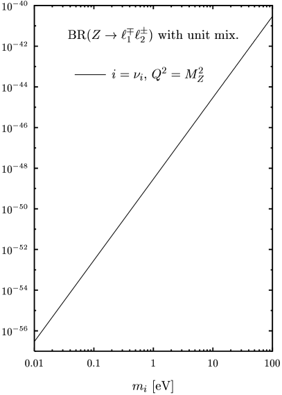
Figure 3: Contribution of one neutrino generation $i$ to the LFV $Z\to\ell_{1}^{\mp}\ell_{2}^{\pm}$ decays for ordinary Dirac neutrinos in the small and large neutrino mass regions, and the analogous quark case. The mixing factor has been set to ${\bf V}_{l_{1}i}{\bf V}^{*}_{l_{2}i}=1$.

This behaviour is shown in Figure 3. It is valid over a large mass range until about $m_{i}\approx 30$ GeV, i.e. just below the $Z$ mass.

Taking now into account the phenomenological squared mass differences $\lambda_{ij}\equiv\Delta m^{2}_{ij}/M^{2}_{W}$ and the mixing angles (2.12)–(2.16), one can determine the finite expectation:

$${\rm BR}(Z\to\mu^{\mp}\tau^{\pm})\simeq 3\times 10^{-6}\times|s^{2}_{12}\lambda_{12}-\lambda_{23}|^{2}\approx(1\div 30)\times 10^{-55},$$ (2.21)

and the upper limit:

$${\rm BR}(Z\to e^{\mp}\mu^{\pm})\simeq{\rm BR}(Z\to e^{\mp}\tau^{\pm})\approx 6\times 10^{-6}\times c^{2}_{12}s^{2}_{12}\lambda^{2}_{12}\raisebox{-3.69899pt}{~{}\shortstack{$<$ \\ [-0.07cm] $\sim$}}~{}4\times 10^{-60}.$$ (2.22)

These extremely small rates are far beyond experimental verification. This justifies taking the light neutrino sector as massless in the following sections where we discuss extensions providing larger rates.

2.2 Contributions from one heavy ordinary Dirac neutrino

Assume the neutrino of generation $N$ to be the only heavy one, mixing with a light sector with negligible masses. Then, using again the unitarity of the mixing matrix:

$${\rm BR}(Z\to\ell_{1}^{\mp}\ell_{2}^{\pm}) = \frac{\alpha_{W}^{3}M_{Z}}{192\pi^{2}c_{W}^{2}\Gamma_{Z}}\left|{\bf V}_{\ell_{1}N}{\bf V}_{\ell_{2}N}^{*}\right|^{2}\left|V_{Z}(\lambda_{N};\lambda_{Z})-V_{Z}(0;\lambda_{Z})\right|^{2}.$$ (2.23)

In the large Dirac neutrino mass limit, the following approximation works well (see Appendix A.2):

$$V_{Z}(\lambda;\lambda_{Z}) = \frac{1}{2}\Biggl{[}-4c^{2}_{W}\Delta_{\epsilon}+\lambda+\left(3-\frac{\lambda_{Z}}{6}(1-2s_{W}^{2})\right)\ln\lambda$$

$$+~{}\frac{1}{18}\left(-66-\lambda_{Z}+96s_{W}^{2}+5s_{W}^{2}\lambda_{Z}\right)$$

$$+~{}\frac{1}{3}\left(-8+2\lambda_{Z}-32s_{W}^{2}-4s_{W}^{2}\lambda_{Z}\right)y\arctan\left(\frac{1}{2y}\right)\Biggr{]}+{\cal O}\left(\frac{\ln\lambda}{\lambda}\right),$$

with

$$y = \sqrt{1/\lambda_{Z}-1/4}.$$ (2.25)

The vertex function contains a constant term proportional to $\Delta_{\epsilon}=2/(4-d)+\gamma+\ln 4\pi$, divergent in $d=4$ dimensions. This term drops out in the physical amplitude, as expected, since the unitarity of the mixing matrix demands the subtraction of $V_{Z}(0;\lambda_{Q})$, with identical divergences. Its expression can be found in Appendix A.1. For an on-shell $Z$,

$$V_{Z}(\lambda_{N};\lambda_{Z})-V_{Z}(0;\lambda_{Z})=\frac{1}{2}\left[\lambda_{N}+2.88\ln\lambda_{N}-(6.99+2.11\ i)\right]+{\cal O}(\ln\lambda_{N}/\lambda_{N}).\hskip 11.38109pt$$ (2.26)

The exact results are depicted in Figure 3, where the simpler calculation with $Q^{2}=0$ [52] is also displayed. We find agreement with earlier calculations [19], also for quark flavour-changing $Z$ decays [21, 22]. Of course, the results for $Q^{2}=0$ are a good approximation only when $m_{N}^{2}\gg M_{Z}^{2}$.

For a study of the size of the branching ratios, the knowledge of the light-heavy mixing elements involved in (2.23) is crucial. Their values do not only influence potential LFV processes but also flavour-diagonal ones. Using a general formalism developed in [53] one can exploit measurements of flavour diagonal processes (checks of lepton universality and CKM unitarity, $Z$ boson invisible width, etc.) [54, 55] to obtain indirect experimental bounds on such light-heavy mixings [56], defined as

$$s^{2}_{\nu_{\ell}}\equiv|\sum_{i}{\bf V}_{\ell N_{i}}|^{2}.$$ (2.27)

The most recent indirect bounds [57]:

$$s^{2}_{\nu_{e}} < 0.012,$$ (2.28)

$$s^{2}_{\nu_{\mu}} < 0.0096,$$ (2.29)

$$s^{2}_{\nu_{\tau}} < 0.016,$$ (2.30)

are only improved by the impressive accuracy of the direct searches for LFV processes involving the first two lepton generations. In fact, for heavy enough neutrinos one can rewrite (1.10):

$${\rm BR}(\mu\to e\gamma)\approx\frac{3\alpha}{8\pi}s^{2}_{\nu_{e}}s^{2}_{\nu_{\mu}},$$ (2.31)

and from (1.2) a stringent ‘mass-independent’ limit can be extracted [58]:

$$s^{2}_{\nu_{e}}s^{2}_{\nu_{\mu}}<1.4\times 10^{-8}.$$ (2.32)

The limit above sends the $Z\to e\mu$ process beyond any experimental reach, even if the neutrinos are very heavy. At this point, it is important to realize that, although the branching fractions for large neutrino masses grow as

$${\rm BR}(Z\to\ell_{1}\ell_{2})\propto s^{2}_{\nu_{\ell_{1}}}s^{2}_{\nu_{\ell_{2}}}m^{4}_{N},$$ (2.33)

there is a ‘natural’ upper value for the neutrino mass determined by the perturbative unitarity condition on the heavy Dirac neutrino decay width [59, 60, 61, 62, 63],

$$\Gamma_{N_{i}}\simeq\frac{\alpha_{W}}{8M^{2}_{W}}m^{3}_{N_{i}}\sum_{\ell}|{\bf V}_{\ell N_{i}}|^{2}\leq\frac{1}{2}m_{N_{i}},$$ (2.34)

that implies

$$m^{2}_{N} \leq \frac{4M^{2}_{W}}{\alpha_{W}}\left[\sum^{3}_{k=1}s^{2}_{\nu_{k}}\right]^{-1}\approx(4.4\ \mbox{TeV})^{2}.$$ (2.35)

In other words, expression (2.34) shows that the unacceptable large-mass behaviour of the amplitudes ($\propto m^{2}_{N}$) is actually cured when a sensible light-heavy mixing (at most $\propto m^{-2}_{N}$) is taken into account [64, 65].

Figure 4: Upper limit of BR$(Z\to\mu^{\mp}\tau^{\pm})$ assuming a light neutrino sector mixing with: (i) one heavy ordinary (thick-solid) or singlet (thin-solid) Dirac neutrino of mass $m_{N_{1}}$; (ii) two heavy right-handed singlet Majorana neutrinos (dashed lines) with masses $m_{N_{1}}$ and $m_{N_{2}}$.

For illustration, we show the less constrained results for $Z\to\mu^{\mp}\tau^{\pm}$ in Figure 4 (thick-solid line), assuming the present (indirect) upper bounds on the corresponding mixings (2.29) and (2.30): given the heavy neutrino mass(es), the branching fractions cannot exceed either the curves or the collider exclusion limit. Regions below the curves correspond to mixings smaller than the upper bounds (2.28) to (2.30). Masses beyond the end points are acceptable only if the mixings are smaller than the upper bounds. Of course, since there are at least two unknowns, a neutrino mass and a combination of mixings, the LFV $Z$ decays cannot improve the bounds on the mixings without assuming a value for the heavy neutrino mass(es). This is in contrast to the LFV $\mu$ decays for sufficiently heavy neutrinos (2.31).

3 The LFV $Z$ decays in the $\nu$SM with right-handed Majorana singlets

Let us now consider the case when the heavy neutrinos are Majorana particles. Actually this a very interesting possibility since such states belong to the particle content of most GUT theories, like SO(10). Furthermore, they may participate in the seesaw mechanism, that explains the smallness of the observed neutrino masses by introducing a general Majorana neutrino [66] mass matrix, incorporating ordinary Dirac mass terms $m_{D}$, of a size typical to the charged lepton sector, and lepton-number violating Majorana mass terms at a higher scale $M_{R}\gg m_{D}$. Majorana mass terms $M_{R}\overline{\nu^{c}_{R}}\nu_{R}+\mbox{h.c.}$, with $\nu_{R}$ being right-handed singlets under the SM group, are gauge invariant, but violate lepton number by two units. The physical states after diagonalization of the mass matrix are, respectively, light and heavy Majorana neutrinos with masses

$$m_{\nu}\approx m^{2}_{D}/M_{R},\quad m_{N}\approx M_{R}\gg m_{\nu}.$$ (3.1)

If there is only one generation of heavy neutrinos, the light-heavy mixings are fixed to be very small,

$$s_{\nu}\approx m_{D}/M_{R}\approx\sqrt{m_{\nu}/m_{N}},$$ (3.2)

leading to unobservable LFV effects.

But this is not the case when one includes several right-handed Majorana neutrinos with inter-generation mixings [67, 68, 56]. We will focus on the most conservative case of two heavy right-handed singlets.

3.1 LFV with Majorana neutrinos

Let us consider $n_{G}$ generations of charged leptons (Dirac fermions), whose left-handed components ($\ell^{0}_{L}=e_{L},\mu_{L},\tau_{L},\dots$) belong to the same isodoublet as $n_{G}$ left-handed neutrinos ($\nu^{0}_{L}=\nu_{e},\nu_{\mu},\nu_{\tau},\dots$) and, in addition, $n_{R}$ right-handed neutrino singlets. The interaction eigenstates are a mixture of physical states given by [69, 70, 56]

$${\ell^{0}_{L}}_{i} = \displaystyle\sum_{j=1}^{n_{G}}{\bf U}^{\ell_{L}}_{ij}\ {\ell_{L}}_{j},$$ (3.3)

$${\nu^{0}_{L}}_{i} = \displaystyle\sum_{j=1}^{n_{G}+n_{R}}{\bf U}_{ij}\ {\nu_{L}}_{j},$$ (3.4)

where $\nu$=$\eta\ \nu^{c}$ are $n_{G}+n_{R}$ Majorana fields (i.e. self-conjugate up to a phase $\eta$).

In the charged-current interactions, one must replace the leptonic mixing matrix ${\bf V}$ by its generalized version, the rectangular $n_{G}\times(n_{G}\times n_{R})$ matrix ${\bf B}$,

$${\bf B}_{ij}\equiv\displaystyle\sum^{n_{G}}_{k=1}{\bf U}^{\ell^{*}_{L}}_{ki}{\bf U}_{kj}.$$ (3.5)

Therefore, in the physical basis,

$$-{\cal L}_{CC} = \frac{g}{\sqrt{2}}W_{\mu}\overline{\ell^{0}_{L}}_{i}\gamma^{\mu}P_{L}{\nu^{0}_{L}}_{i}+h.c.$$ (3.6)

$$= \frac{g}{\sqrt{2}}W_{\mu}\ {\bf B}_{ij}\ \overline{\ell_{L}}_{i}\gamma^{\mu}P_{L}{\nu_{L}}_{j}+h.c.,$$

where $P_{R,L}=\frac{1}{2}(1\pm\gamma_{5})$.

But the main feature distinguishing Dirac and Majorana cases is the existence of non-diagonal $Z\nu_{i}\nu_{j}$ vertices (flavour-changing neutral current), coupling both left- and right-handed components of the Majorana mass eigenstates to the $Z$ boson,

$$-{\cal L}^{Z}_{NC} = \frac{g}{2c_{W}}Z_{\mu}[\overline{\nu^{0}_{L}}_{i}\gamma^{\mu}P_{L}{\nu^{0}_{L_{i}}}-\overline{\nu^{0c}_{L}}_{i}\gamma^{\mu}P_{R}{\nu^{0c}_{L_{i}}}]$$ (3.7)

$$= \frac{g}{2c_{W}}Z_{\mu}\overline{\nu_{i}}[{\bf C}_{ij}\gamma^{\mu}P_{L}-{\bf C}^{*}_{ij}\gamma^{\mu}P_{R}]\nu_{j},$$

where $\nu^{0c}_{L}=C\overline{\nu^{0}_{L}}^{T}$ is the charge-conjugate of $\nu^{0}_{L}$, which is right-handed, and

$${\bf C}_{ij}\equiv\displaystyle\sum^{n_{G}}_{k=1}{\bf U}^{*}_{ki}{\bf U}_{kj},\quad(i,j=1,\dots,n_{G}+n_{R}),$$ (3.8)

a quadratic $(n_{G}+n_{R})^{2}$ matrix. Such flavour-changing NC vertices appear in graphs D1 and D3 of Figure 2 where Majorana neutrinos couple directly to the $Z$, and a $W$ or a Goldstone boson $\phi$ is exchanged:

$$v_{W}(i,j) = -{\bf C}_{ij}\big{[}\lambda_{Q}({\mathbb{C}}_{0}+{\mathbb{C}}_{11}+{\mathbb{C}}_{12}+{\mathbb{C}}_{23})-2{\mathbb{C}}_{24}+1\big{]}+{\bf C}^{*}_{ij}\sqrt{\lambda_{i}\lambda_{j}}\ {\mathbb{C}}_{0},$$ (3.9)

$$v_{\phi}(i,j) = -{\bf C}_{ij}\displaystyle\frac{\lambda_{i}\lambda_{j}}{2}{\mathbb{C}}_{0}+{\bf C}^{*}_{ij}\displaystyle\frac{\sqrt{\lambda_{i}\lambda_{j}}}{2}\left[\lambda_{Q}{\mathbb{C}}_{23}-2{\mathbb{C}}_{24}+\displaystyle\frac{1}{2}\right].$$ (3.10)

The other diagrams remain unchanged compared to the Dirac case and the resulting form factor reads:

$${\cal V}_{\rm Maj}(Q^{2}) = \sum^{n_{G}+n_{R}}_{i,j=1}{\bf B}_{\ell_{1}i}{\bf B}^{*}_{\ell_{2}j}V_{Z}(i,j),$$ (3.11)

$$V_{Z}(i,j) = v_{W}(i,j)+v_{\phi}(i,j)+v_{WW}(i)+v_{\phi\phi}(i)+v_{W\phi}(i)+v_{\Sigma}(i).$$ (3.12)

We have used the Feynman rules in [72, 73] to properly handle interactions involving Majorana particles.

It turns out convenient to cast (3.12) as

$$V_{Z}(\lambda_{i},\lambda_{j}) = \delta_{ij}F(\lambda_{i})+{\bf C}_{ij}G(\lambda_{i},\lambda_{j})+{\bf C}^{*}_{ij}\sqrt{\lambda_{i}\lambda_{j}}H(\lambda_{i},\lambda_{j}).$$ (3.13)

The Dirac vertex function (2.3) is then

$$V_{Z}(\lambda_{i})=F(\lambda_{i})+G(\lambda_{i},\lambda_{i}).$$ (3.14)

The form factor (3.11) is UV-finite, but the vertex function $V_{Z}(\lambda_{i},\lambda_{j})$ is not. The divergences are such that they exactly cancel due to unitarity relations among the mixing matrix elements of ${\bf B}$ and ${\bf C}$ [56, 27]. The same relations allow to write ${\cal V}_{\rm Maj}$ in terms of only the heavy sector, assuming the light sector being massless:

$${\cal V}_{\rm Maj}(Q^{2}) = \sum^{n_{R}}_{i,j=1}{\bf B}_{\ell_{1}N_{i}}{\bf B}^{*}_{\ell_{2}N_{j}}$$ (3.15)

$$\times~{}\Big{\{}\delta_{N_{i}N_{j}}[\ F(\lambda_{N_{i}})-F(0)+G(\lambda_{N_{i}},0)+G(0,\lambda_{N_{i}})-2G(0,0)]$$

$$+~{}{\bf C}_{N_{i}N_{j}}[\ G(\lambda_{N_{i}},\lambda_{N_{j}})-G(\lambda_{N_{i}},0)-G(0,\lambda_{N_{j}})+G(0,0)]$$

$$+~{}{\bf C}^{*}_{N_{i}N_{j}}\sqrt{\lambda_{N_{i}}\lambda_{N_{j}}}\ H(\lambda_{N_{i}},\lambda_{N_{j}})\Big{\}}.$$

3.2 The $\nu$SM with two heavy Majorana singlets

In the simple case of $n_{R}=2$ heavy right-handed singlet neutrinos $N_{1}$ and $N_{2}$, mixing with a massless sector, the ${\bf B}$ and ${\bf C}$ matrices are fully determined by the ratio of the two physical heavy masses squared $r\equiv m^{2}_{N_{2}}/m^{2}_{N_{1}}$ and the light-heavy mixings $s^{2}_{\nu_{\ell}}$, here

$$s^{2}_{\nu_{\ell}}\equiv\sum_{i}|{\bf B}_{\ell N_{i}}|^{2}.$$ (3.16)

Their explicit values are [56]:

$${\bf B}_{\ell N_{1}} = \frac{r^{1/4}}{\sqrt{1+r^{1/2}}}s_{\nu_{\ell}},$$ (3.17)

$${\bf B}_{\ell N_{2}} = \frac{i}{\sqrt{1+r^{1/2}}}s_{\nu_{\ell}},$$ (3.18)

$${\bf C}_{N_{1}N_{1}} = \frac{r^{1/2}}{1+r^{1/2}}\sum_{\ell}s^{2}_{\nu_{\ell}},$$ (3.19)

$${\bf C}_{N_{2}N_{2}} = \frac{1}{1+r^{1/2}}\sum_{\ell}s^{2}_{\nu_{\ell}},$$ (3.20)

$${\bf C}_{N_{1}N_{2}}\ =\ -~{}{\bf C}_{N_{2}N_{1}} = \frac{ir^{1/4}}{1+r^{1/2}}\sum_{\ell}s^{2}_{\nu_{\ell}}.$$ (3.21)

The mass ratio $r$ is a free parameter and the light-heavy mixings are constrained by present experiments as shown in Section 2.2. Upper values for the branching ratios of $Z\to\mu^{\mp}\tau^{\pm}$, obtained from the experimental bounds given the heavy masses $m_{N_{1}}$, $m_{N_{2}}$, are also displayed in Figure 4.

The case of two equal-mass Majorana neutrinos $m_{N_{1}}=m_{N_{2}}$ is equivalent to one heavy singlet Dirac neutrino, and it approaches rapidly the ordinary Dirac case for small masses. This phenomenon is just another example of the “practical Dirac-Majorana confusion theorem” [74] (see also the recent discussion in [75, 76] and references therein). If both masses $m_{N_{1}}$ and $m_{N_{2}}$ are small, the amplitude goes as $\sqrt{r}\lambda_{N_{1}}=m_{N_{1}}m_{N_{2}}/M^{2}_{W}$ with the same global factor $a_{1}$ as in the ordinary Dirac case (2.20). This can been seen in Figure 4 not far below the $Z$ peak, where the branching ratios grow with $\lambda^{2}_{N_{1}}$ and scale with the ratio of the two neutrino masses squared.

If one of the neutrinos has the mass of the $Z$ boson, the imaginary parts of the amplitudes ${\cal V}_{\rm Dir,Maj}$ (coming from the subtraction(s) at $\lambda_{N}=0$) dominates, both for the Dirac and the Majorana cases. This happens since the real parts are slowly varying for $M_{N}\leq M_{Z}$, while the imaginary parts vanish for $M_{Z}<M_{N}+M_{N^{\prime}}$. Further, since these imaginary parts necessarily come from accounting the subtractions of the zero mass limits, they are independent of the value of $r$. This results in common values of the branching ratios for $m_{N_{1}}=M_{Z}$ for any value of $m_{N_{2}}$. Nevertheless, the subtraction of the light sector implied by the unitarity constraints is not the same for the cases of a heavy ordinary Dirac neutrino and heavy Majorana singlets. One finds explicitly

$$\frac{\Im{\rm m}({\cal V}_{\rm Dir})}{s_{\nu_{\ell_{1}}}s_{\nu_{\ell_{2}}}}=-1.0524,\quad\frac{\Im{\rm m}({\cal V}_{\rm Maj})}{s_{\nu_{\ell_{1}}}s_{\nu_{\ell_{2}}}}=-2.0653.$$ (3.22)

The expansion of the form factor (3.15) in the large neutrino mass limit $\lambda_{N_{1}}\gg 1$, at fixed $r$, leads to (see Appendix A.2):

$${\cal V}_{\rm Maj}(Q^{2}) = s_{\nu_{\ell_{1}}}s_{\nu_{\ell_{2}}}\Bigg{\{}\frac{\sum_{\ell}s^{2}_{\nu_{\ell}}}{(1+r^{\frac{1}{2}})^{2}}\left(\frac{3}{2}r+\frac{r^{2}+r-4r^{\frac{3}{2}}}{4(1-r)}\ln r\right)\lambda_{N_{1}}$$ (3.23)

$$+~{}\frac{1}{2}\left(3-\frac{1-2s^{2}_{W}}{6}\lambda_{Q}\right)\ln\lambda_{N_{1}}\Bigg{\}}+{\cal O}(1),$$

that agrees with [56] for the unphysical value $\lambda_{Q}=0$. The constant in front of the leading term coincides for $r=1$ with the ordinary Dirac case, except for an extra damping factor $\sum_{\ell}s^{2}_{\nu_{\ell}}$, that makes the Dirac singlet case in particular, and the Majorana case in general, more sensitive to the present bounds on the light-heavy mixings. The constant in front of the $\ln\lambda$ term, subleading but not so much mixing-suppressed, is identical to the one in the ordinary Dirac case (2.2).

We have cut again the curves at the perturbative unitarity mass limits. Due to the different number of degrees of freedom of the Majorana particles, the condition on the heavy neutrino width is this time [62],

$$\Gamma_{N_{i}}\simeq 2\times\frac{\alpha_{W}}{8M^{2}_{W}}m^{3}_{N_{i}}\sum_{\ell}|{\bf B}_{\ell N_{i}}|^{2}\leq\frac{1}{2}m_{N_{i}},$$ (3.24)

resulting in the mass limits

$$m^{2}_{N_{1}}\equiv\frac{1}{r}m^{2}_{N_{2}} < \sim \frac{1+r^{1/2}}{r}\times(3.1\ \mbox{TeV})^{2}.$$   [-0.07cm] (3.25)

We see from the figure that GigaZ has a discovery potential, preferentially in the large neutrino mass region, if the light heavy-mixings are not much below the present upper limits. Due to the different coupling structure, the simple sequential Dirac neutrino case does not constitute a limiting case for large masses.

4 Concluding remarks

The sensitivity of the GigaZ mode of the future TESLA linear collider to rare, lepton-flavour violating $Z$ decays has been studied. We have determined the full one-loop expectations for the direct lepton-flavour changing process $Z\to\bar{\ell}_{1}\ell_{2}$ with virtual Dirac or Majorana neutrinos. This is an interesting theoretical issue in view of the evidences for tiny neutrino masses from astrophysics, which might be also indicative for the existence of heavy neutrinos in some Grand Unifying Theory. Both the exact analytical form and the large and small neutrino mass limits of the branching ratios are given, thereby cross-checking the existing literature. From our numerical studies, taking into account the present experimental results, we conclude that: (i) the contributions from the observed light neutrino sector are far from experimental verification (BR$\raisebox{-3.69899pt}{~{}\shortstack{$<$ \\ [-0.07cm] $\sim$}}~{}10^{-54}$); (ii) the GigaZ mode of the future TESLA linear collider, sensitive down to about BR $\sim 10^{-8}$, might well have a chance to produce such processes, if heavy neutrinos exist in Nature and if they mix with the light ones in a sizeable way. Finally, we have shown that we could gain from observation of the LFV $Z$ decays alternative informations compared to the LFV $\mu$ decays.

Appendix A Tensor integrals and vertex functions

We have introduced dimensionless two- and three-point one-loop functions:

$${{\mathbb{B}}}_{1}(\lambda_{i}) \equiv B_{1}(0;m^{2}_{i},M^{2}_{W}),$$ (A.1)

$$\bar{{\mathbb{C}}}_{..}(\lambda_{i}) \equiv M^{2}_{W}\ C_{..}(0,Q^{2},0;m^{2}_{i},M^{2}_{W},M^{2}_{W}),$$ (A.2)

$${\mathbb{C}}_{..}(\lambda_{i},\lambda_{j}) \equiv M^{2}_{W}\ C_{..}(0,Q^{2},0;M^{2}_{W},m^{2}_{i},m^{2}_{j}),$$ (A.3)

from the usual loop integrals [14, 77] with the tensor decomposition (Minkowski metric):

$$B^{\mu}(p^{2};m^{2}_{0},m^{2}_{1}) = p^{\mu}B_{1},$$ (A.4)

$$C^{\mu}(p^{2}_{1},Q^{2},p^{2}_{2};m^{2}_{0},m^{2}_{1},m^{2}_{2}) = p^{\mu}_{1}C_{11}+p^{\mu}_{2}C_{12},$$ (A.5)

$$C^{\mu\nu}(p^{2}_{1},Q^{2},p^{2}_{2};m^{2}_{0},m^{2}_{1},m^{2}_{2}) = p^{\mu}_{1}p^{\nu}_{1}C_{21}+p^{\mu}_{2}p^{\nu}_{2}C_{22}+(p^{\mu}_{1}p^{\nu}_{2}+p^{\mu}_{2}p^{\nu}_{1})C_{23}+g^{\mu\nu}M^{2}_{W}C_{24}.$$

The tensor integrals are numerically evaluated with the computer program LoopTools [78], based on FF [79]. All the numerical results for the Dirac case have been carefully checked against an older approach described in [19].

The following definitions of the integrals in $d$ dimensions are useful:

$${\mathbb{B}}_{1}(\lambda_{i}) = -\frac{\Delta_{\epsilon}}{2}+\int_{0}^{1}dx\ x\ln[(1-\lambda_{i})x+\lambda_{i}-i\epsilon],$$ (A.7)

$${\mathbb{C}}_{24}(\lambda_{i},\lambda_{j}) = \frac{\Delta_{\epsilon}}{4}-\frac{1}{2}\int_{0}^{1}dx\int_{0}^{x}dy~{}\ln D_{ijW},$$ (A.8)

$${\mathbb{C}}_{0,11,23}(\lambda_{i},\lambda_{j}) = -\int_{0}^{1}dx\int_{0}^{x}dy~{}[1,-y,y(1-x)]~{}\frac{1}{D_{ijW}},$$ (A.9)

with $\lambda_{i}=m^{2}_{i}/M^{2}_{W}$, $\Delta_{\epsilon}=2/(4-d)-\gamma+\ln 4\pi$ and

$$D_{ijW}\equiv \lambda_{Z}xy+(1-\lambda_{j})x+[-\lambda_{Z}+(\lambda_{i}-1)]y+\lambda_{j}-i\epsilon.$$ (A.10)

To get the barred tensor integrals $\bar{\mathbb{C}}$, replace $D_{ijW}$ by:

$$D_{WWi}\equiv\lambda_{Z}xy-(1-\lambda_{i})x+[-\lambda_{Z}-(\lambda_{i}-1)]y+1-i\epsilon.$$ (A.11)

The functions ${\mathbb{B}}_{1}$, ${\mathbb{C}}_{24}$ and $\bar{\mathbb{C}}_{24}$ are UV-divergent but the physical amplitudes are finite.

A.1 Light neutrino mass expansions

Let us first list the value of the necessary tensor integrals for massless neutrinos and $\lambda_{Q}\neq 0$ [19]:

$${\mathbb{B}}_{1}(0) = -\frac{\Delta_{\epsilon}}{2}-\frac{1}{4},$$ (A.12)

$${\mathbb{C}}_{0}(0,0) = -c_{0},$$ (A.13)

$${\mathbb{C}}_{11}(0,0) = -\frac{1}{\lambda_{Q}}(c_{0}-1+\ln\lambda_{Q}-i\pi),$$ (A.14)

$${\mathbb{C}}_{12}(0,0) = {\mathbb{C}}_{11}(0,0),$$ (A.15)

$${\mathbb{C}}_{23}(0,0) = -\frac{1}{\lambda_{Q}^{2}}\left[(\lambda_{Q}+2)c_{0}-\frac{\lambda_{Q}}{2}-2+2(\ln\lambda_{Q}-i\pi)\right],$$ (A.16)

$${\mathbb{C}}_{24}(0,0) = \frac{\Delta_{\epsilon}}{4}+\frac{1}{4\lambda_{Q}}[-2(\lambda_{Q}+1)c_{0}+3\lambda_{Q}+2-(\lambda_{Q}+2)(\ln\lambda_{Q}-i\pi)],\hskip 11.38109pt$$ (A.17)

$$\bar{\mathbb{C}}_{0}(0) = -\bar{c}_{0},$$ (A.18)

$$\bar{\mathbb{C}}_{11}(0) = \frac{1}{\lambda_{Q}}(\bar{c}_{0}-B+1),$$ (A.19)

$$\bar{\mathbb{C}}_{12}(0) = \bar{\mathbb{C}}_{11}(0),$$ (A.20)

$$\bar{\mathbb{C}}_{23}(0) = -\frac{2}{\lambda_{Q}^{2}}\left(\bar{c}_{0}-B+1-\frac{\lambda_{Q}}{4}\right),$$ (A.21)

$$\bar{\mathbb{C}}_{24}(0) = \frac{\Delta_{\epsilon}}{4}-\frac{1}{2\lambda_{Q}}\left[\bar{c}_{0}-B+1-\frac{3}{2}\lambda_{Q}+\pi\lambda_{Q}y-2\lambda_{Q}y\arctan(2y)\right],$$ (A.22)

with

$$\lambda_{Q}~{}c_{0} = \frac{\pi^{2}}{6}-\mbox{Li}_{2}\left(\frac{1}{1+\lambda_{Q}}\right)-\frac{1}{2}\ln^{2}(1+\lambda_{Q})+\pi\ln(1+\lambda_{Q})\ i,$$ (A.23)

$$\lambda_{Q}~{}{\bar{c}}_{0} = \frac{\pi^{2}}{6}-\mbox{Li}_{2}(1-\lambda_{Q})+2\Re e\mbox{Li}_{2}\left[(\lambda_{Q}-1)\left(\frac{\lambda_{Q}}{2}-1+\lambda_{Q}y\ i\right)\right]$$ (A.24)

$$-~{}2\Re e\mbox{Li}_{2}\left(1-\frac{\lambda_{Q}}{2}-\lambda_{Q}y\ i\right),$$

$$B = 2y\left[\arctan(2y)+\arctan\left(\frac{\lambda_{Q}-1}{3-\lambda_{Q}}2y\right)\right].$$ (A.25)

After expanding the tensor integrals for small neutrino masses (see Appendix D.2 of [27]), the vertex function for the case of a light Dirac neutrino reads:

$$V_{Z}(\lambda\ll 1;\lambda_{Q}\neq 0) = V_{Z}(0;\lambda_{Q})+a_{1}\lambda+{\cal O}(\lambda^{2}),$$ (A.26)

where the terms proportional to $\lambda\ln\lambda$ have cancelled out and

$$V_{Z}(0;\lambda_{Q}) = -2c^{2}_{W}\Delta_{\epsilon}+\frac{2+3\lambda_{Q}}{2\lambda_{Q}}(\ln\lambda_{Q}-\pi\ i)-\frac{1}{4\lambda_{Q}^{2}}(7\lambda_{Q}^{2}+14\lambda_{Q}-8)\frac{(1+\lambda_{Q})^{2}}{\lambda_{Q}}c_{0}$$ (A.27)

$$+~{}\frac{2}{\lambda_{Q}^{2}}(1+2\lambda_{Q})({\bar{c}}_{0}-B)+\frac{6}{\lambda_{Q}}[\pi y-2y\arctan(2y)].\hskip 22.76219pt$$

Only the functions ${\bar{\mathbb{C}}}_{..}$ develop imaginary parts, and only for $\lambda_{Q}>4\lambda_{i}$. At the $Z$ peak the numerical result is:

$$V_{Z}(0;\lambda_{Z}) = -2c^{2}_{W}\Delta_{\epsilon}+1.2584+1.0524\ i.$$ (A.28)

The linear term in the expansion (A.26) has the coefficient [18, 27, 28]:

$$a_{1}(\lambda_{Z}) = -\frac{2}{\lambda_{Z}}(1+\lambda_{Z})c_{0}+\frac{1}{2\lambda_{Z}^{2}}(4\lambda_{Z}^{2}-5\lambda_{Z}-6){\bar{c}}_{0}-\frac{2}{\lambda_{Z}}(\ln\lambda_{Z}-\pi\ i)$$ (A.29)

$$+~{}\frac{1}{8\lambda_{Z}^{2}}(25\lambda_{Z}^{2}-38\lambda_{Z}-24)+\frac{1}{2\lambda_{Z}}(2-\lambda_{Z})\pi y$$

$$+~{}\frac{1}{\lambda_{Z}^{2}}(\lambda_{Z}^{2}+7\lambda_{Z}+6)y\arctan(2y)$$

$$+~{}\frac{3}{\lambda_{Z}^{2}}(3\lambda_{Z}+2)y\arctan\left(\frac{\lambda_{Z}-1}{3-\lambda_{Z}}2y\right)$$

$$= 2.5623-2.2950\ i.$$ (A.30)

The behaviour of (A.26) is in contrast to the case $\lambda_{Q}=0$ for which [52, 19, 27]:

$$V_{Z}(\lambda\ll 1;\lambda_{Q}=0)=\frac{1}{2}(-4c^{2}_{W}\Delta_{\epsilon}+6\lambda+2\lambda\ln\lambda)+{\cal O}(\lambda^{2}).$$ (A.31)

A.2 Heavy neutrino mass expansions

The limits of the necessary tensor integrals and the vertex function in the Dirac case for large neutrino masses can be found in Appendix D of [27]. We collect below the large mass expansions of the tensor integrals that are also needed for the Majorana case, namely one or two identical neutrinos running in the loop:

$${\mathbb{B}}_{1}(\lambda_{i}) = -\frac{\Delta_{\epsilon}}{2}+\frac{1}{2}\ln\lambda_{i}-\frac{3}{4}+\frac{\ln\lambda_{i}}{\lambda_{i}}-\frac{1}{2\lambda_{i}}+{\cal O}(1/\lambda_{i}^{2}),$$ (A.32)

$$\bar{\mathbb{C}}_{0}(\lambda_{i}) = -\frac{\ln\lambda_{i}}{\lambda_{i}}-\left[1-4y\arctan\left(\frac{1}{2y}\right)\right]\frac{1}{\lambda_{i}}+{\cal O}(1/\lambda_{i}^{3}),$$ (A.33)

$$\bar{\mathbb{C}}_{11}(\lambda_{i})=\bar{\mathbb{C}}_{12}(\lambda_{i}) = \frac{1}{2}\frac{\ln\lambda_{i}}{\lambda_{i}}+{\cal O}(1/\lambda_{i}^{2}),$$ (A.34)

$$\bar{\mathbb{C}}_{23}(\lambda_{i}) = -\frac{1}{6}\frac{\ln\lambda_{i}}{\lambda_{i}}+{\cal O}(1/\lambda_{i}^{2}),$$ (A.35)

$$\bar{\mathbb{C}}_{24}(\lambda_{i}) = \frac{\Delta_{\epsilon}}{4}-\frac{1}{4}\ln\lambda_{i}+\frac{3}{8}+\left(-6+\lambda_{Q}\right)\frac{\ln\lambda_{i}}{12\lambda_{i}}$$ (A.36)

$$+\left[-30+5\lambda_{Q}+24(4-\lambda_{Q})y\arctan\left(\frac{1}{2y}\right)\right]\frac{1}{72\lambda_{i}}$$

$$+{\cal O}(1/\lambda_{i}^{2}),$$

$${\mathbb{C}}_{0}(\lambda_{i},\lambda_{i}) = -\frac{1}{\lambda_{i}}+\frac{\ln\lambda_{i}}{\lambda_{i}^{2}}-\left(12+\lambda_{Q}\right)\frac{1}{12\lambda_{i}^{2}}+{\cal O}(1/\lambda_{i}^{3}),$$ (A.37)

$${\mathbb{C}}_{11}(\lambda_{i},\lambda_{i})={\mathbb{C}}_{12}(\lambda_{i},\lambda_{i}) = \frac{1}{4\lambda_{i}}+{\cal O}(1/\lambda_{i}^{2}),$$ (A.38)

$${\mathbb{C}}_{23}(\lambda_{i},\lambda_{i}) = -\frac{1}{18\lambda_{i}}+{\cal O}(1/\lambda_{i}^{2}),$$ (A.39)

$${\mathbb{C}}_{24}(\lambda_{i},\lambda_{i}) = \frac{\Delta_{\epsilon}}{4}-\frac{1}{4}\ln\lambda_{i}+\frac{1}{8}+\left(-9+\lambda_{Q}\right)\frac{1}{36\lambda_{i}}+{\cal O}(1/\lambda_{i}^{2}),\hskip 22.76219pt$$ (A.40)

with

$$y=\sqrt{1/\lambda_{Q}-1/4}.$$ (A.41)

Substituting the expressions above in (2.3) one gets the Dirac vertex function of (2.2).

Besides, we need some additional expansions for two Majorana fermions with different large masses masses $\lambda_{i}\neq\lambda_{j}$,

$${\mathbb{C}}_{0}(\lambda_{i},\lambda_{j}) = -\frac{1}{\lambda_{i}-\lambda_{j}}\left[\frac{\lambda_{i}}{\lambda_{i}-1}\ln\lambda_{i}-\frac{\lambda_{j}}{\lambda_{j}-1}\ln\lambda_{j}\right]$$ (A.42)

$$+~{}\frac{\lambda_{Q}}{(\lambda_{i}-\lambda_{j})^{2}}\left[1+\frac{1}{2}\left(1-\frac{2\lambda_{i}}{\lambda_{i}-\lambda_{j}}\right)\ln\lambda_{i}+\frac{1}{2}\left(1+\frac{2\lambda_{j}}{\lambda_{i}-\lambda_{j}}\right)\ln\lambda_{j}\right]$$

$$+~{}{\cal O}(1/\lambda^{3}),$$

and, to a lower accuracy in the expansion parameters:

$${\mathbb{C}}_{11}(\lambda_{i},\lambda_{j}) = \frac{1}{2}\frac{1+\ln\lambda_{i}}{\lambda_{i}-\lambda_{j}}+\frac{\lambda_{j}\ln\lambda_{j}-\lambda_{i}\ln\lambda_{i}}{2(\lambda_{i}-\lambda_{j})^{2}}+{\cal O}(1/\lambda^{2}),$$ (A.43)

$${\mathbb{C}}_{12}(\lambda_{i},\lambda_{j}) = {\mathbb{C}}_{11}(\lambda_{j},\lambda_{i}),$$ (A.44)

$${\mathbb{C}}_{23}(\lambda_{i},\lambda_{j}) = -\frac{1}{6(\lambda_{i}-\lambda_{j})^{2}}\left[(\lambda_{i}+\lambda_{j})-\frac{2\lambda_{i}\lambda_{j}}{\lambda_{i}-\lambda_{j}}\left(\ln\lambda_{i}-\ln\lambda_{j}\right)\right]+{\cal O}(1/\lambda^{2}),$$ (A.45)

$${\mathbb{C}}_{24}(\lambda_{i},\lambda_{j}) = \frac{3}{8}-\frac{1}{4}\frac{(\lambda_{i}+1)\ln\lambda_{i}-(\lambda_{j}+1)\ln\lambda_{j}}{\lambda_{i}-\lambda_{j}}-\frac{\lambda_{Q}}{2}{\mathbb{C}}_{23}(\lambda_{i},\lambda_{j})+{\cal O}(1/\lambda^{2}).\hskip 34.1433pt$$ (A.46)

Actually, ${\mathbb{C}}_{11}$ and ${\mathbb{C}}_{12}$ are irrelevant for large neutrino masses.

Finally, in (3.15) we need loop integrals where one neutrino mass is large and the other one vanishes. They are all irrelevant except ${\mathbb{C}}_{24}$ in this limit, but we show their expansions for completeness:

$${\mathbb{C}}_{0}(\lambda,0) = -\frac{\ln\lambda}{\lambda}-\frac{\ln\lambda}{\lambda^{2}}+\frac{\lambda_{Q}}{2\lambda^{2}}+{\cal O}(1/\lambda^{3}),$$ (A.47)

$${\mathbb{C}}_{12}(0,\lambda)={\mathbb{C}}_{11}(\lambda,0) = \frac{1}{2\lambda}+(3+\lambda_{Q})\frac{1}{6\lambda^{2}}-\frac{\ln\lambda}{\lambda^{2}}+{\cal O}(1/\lambda^{3}),$$ (A.48)

$${\mathbb{C}}_{11}(0,\lambda)={\mathbb{C}}_{12}(\lambda,0) = \frac{1}{2\lambda}+(3+2\lambda_{Q})\frac{\ln\lambda}{6\lambda^{2}}+\frac{\lambda_{Q}}{3\lambda^{2}}+{\cal O}(1/\lambda^{3}),$$ (A.49)

$${\mathbb{C}}_{23}(\lambda,0) = -\frac{1}{6\lambda}-(2+\lambda_{Q})\frac{1}{12\lambda^{2}}-\frac{\ln\lambda}{6\lambda^{2}}+{\cal O}(1/\lambda^{3}),$$ (A.50)

$${\mathbb{C}}_{24}(\lambda,0) = \frac{\Delta_{\epsilon}}{2}+\frac{3}{8}-\frac{\ln\lambda}{4}-\frac{\lambda_{Q}}{12\lambda}+{\cal O}(1/\lambda^{2}),$$ (A.51)

and

$${\mathbb{C}}_{0,23,24}(0,\lambda)={\mathbb{C}}_{0,23,24}(\lambda,0).$$ (A.52)

References

- [1] MEGA Collaboration, M. L. Brooks et al., Phys. Rev. Lett. 83 (1999) 1521.
- [2] Particle Data Group Collaboration, C. Caso et al., Eur. Phys. J. C3 (1998) 1–794.
- [3] OPAL Collaboration, R. Akers et al., Z. Phys. C67 (1995) 555–564.
- [4] L3 Collaboration, O. Adriani et al., Phys. Lett. B316 (1993) 427.
- [5] DELPHI Collaboration, P. Abreu et al., Z. Phys. C73 (1997) 243.
- [6] S. L. Glashow, Nucl. Phys. 22 (1961) 579.
- [7] S. Weinberg, Phys. Rev. Lett. 19 (1967) 1264.
- [8] A. Salam, “Weak and Electromagnetic Interactions”, in N. Svartholm (ed.), Elementary Particle Theory, Proceedings of the Nobel Symposium held 1968 at Lerum, Sweden (Almqvist and Wiksell, Stockholm, 1968), pp. 367-377.
- [9] B. Pontecorvo, Zh. Eksp. Teor. Fiz. 33 (1957) 549–551.
- [10] Z. Maki, M. Nakagawa, and S. Sakata, Prog. Theor. Phys. 28 (1962) 870.
- [11] B. Pontecorvo, Sov. Phys. JETP 26 (1968) 984–988.
- [12] M. Veltman, Nucl. Phys. B7 (1968) 637–650.
- [13] G. ’t Hooft, Nucl. Phys. B35 (1971) 167–188.
- [14] G. ’t Hooft and M. Veltman, Nucl. Phys. B44 (1972) 189–213.
- [15] S. Petcov, Sov. J. Nucl. Phys. 25 (1977) 340; E: ibid., 25 (1977) 698.
- [16] T. P. Cheng and L.-F. Li, Phys. Rev. Lett. 38 (1977) 381.
- [17] W. J. Marciano and A. I. Sanda, Phys. Lett. B67 (1977) 303.
- [18] T. Riemann and G. Mann, “Nondiagonal decay: ”, in Proc. of the Int. Conf. Neutrino’82, 14-19 June 1982, Balatonfüred, Hungary (A. Frenkel and E. Jenik, eds.), vol. II, pp. 58–61, Budapest, 1982.
- [19] G. Mann and T. Riemann, Annalen Phys. 40 (1984) 334.
- [20] T. Riemann, “ decay and the quark mass”, in Proc. of the XVIth Int. Symp. Ahrenshoop – Special Topics In Gauge Field Theories, 28 Oct - 4 Nov 1982, Ahrenshoop, GDR (G. Weigt, ed.), pp. 182–190, IfH Zeuthen preprint PHE 82-10 (1982).
- [21] V. Ganapathi, T. Weiler, E. Laermann, I. Schmitt, and P. Zerwas, Phys. Rev. D27 (1983) 579.
- [22] M. Clements, C. Footman, A. Kronfeld, S. Narasimhan, and D. Photiadis, Phys. Rev. D27 (1983) 570.
- [23] S. L. Glashow, J. Iliopoulos, and L. Maiani, Phys. Rev. D2 (1970) 1285.
- [24] W. A. Mann, “Atmospheric neutrinos and the oscillations Bonanza”, Talk at 19th Int. Symp. on Lepton and Photon Interactions at High Energies (LP 99), Stanford, California, 9-14 Aug 1999, hep-ex/9912007.
- [25] J. N. Bahcall, P. I. Krastev, and A. Y. Smirnov, Phys. Rev. D58 (1998) 096016.
- [26] X. Y. Pham, “Is the lepton flavor changing observable in decay?”, Paris Univ. preprint PAR/LPTHE/98-45 (Sept 1998).
- [27] J. I. Illana, M. Jack, and T. Riemann, “Predictions for and related reactions”, DESY Linear Collider Note LC-TH-2000-007 (2000), contrib. to: R. Heuer, F. Richard and P. Zerwas (eds.), Physics Studies for a Future Linear Collider, to appear as report DESY 123F, hep-ph/0001273.
- [28] J. I. Illana and T. Riemann, Nucl. Phys. B (Proc. Suppl.) 89 (2000) 64–69, hep–ph/0006055.
- [29] P. Langacker, Phys. Rept. 72 (1981) 185.
- [30] J. L. Hewett and T. G. Rizzo, Phys. Rept. 183 (1989) 193.
- [31] T. Yanagida, Prog. Theor. Phys. 64 (1980) 1103, also in: O. Sawada and A. Sugamoto (eds.), Proceedings of the Workshop on the Baryon Number of the Universe and Unified Theories, KEK, Tsukuba, Japan, 13-14 Feb 1979, p. 95.
- [32] M. Gell-Mann, P. Ramond, and R. Slansky, “Complex Spinors and Unified Theories”, in: P. van Nieuwenhuizen and D. Friedman (eds.), Proc. of the Workshop on Supergravity, Stony Brook, New York, 27-28 Sep 1979 (North-Holland, Amsterdam, 1979), p. 315-321.
- [33] R. N. Mohapatra and G. Senjanovic, Phys. Rev. Lett. 44 (1980) 912.
- [34] P. Langacker and D. London, Phys. Rev. D38 (1988) 907.
- [35] J. Bernabéu, M. Gavela, and A. Santamaría, Phys. Rev. Lett. 57 (1986) 1514.
- [36] N. Rius and J. W. F. Valle, Phys. Lett. B246 (1990) 249–255.
- [37] M. C. Gonzalez-García, A. Santamaría, and J. W. F. Valle, Nucl. Phys. B342 (1990) 108–126.
- [38] M. Dittmar, A. Santamaría, M. Gonzalez-García, and J. Valle, Nucl. Phys. B332 (1990) 1.
- [39] M. J. Duncan, Phys. Rev. D31 (1985) 1139.
- [40] F. Gabbiani, J. H. Kim, and A. Masiero, Phys. Lett. B214 (1988) 398.
- [41] J. Bernabéu, A. Santamaría, J. Vidal, A. Méndez, and J. Valle, Phys. Lett. B187 (1987) 303.
- [42] F. del Aguila, E. Laermann, and P. Zerwas, Nucl. Phys. B297 (1988) 1.
- [43] P. Langacker and M. Plümacher, Phys. Rev. D62 (2000) 013006.
- [44] W. Bernreuther, M. Duncan, E. Glover, R. Kleiss, J. van der Bij, J. Gomez-Cadenas, and C. Heusch, “Rare decays”, in Physics at LEP 1, CERN 89–08 (1989) (G. Altarelli, R. Kleiss, and C. Verzegnassi, eds.), vol. 2, pp. 1–57.
- [45] E. Blucher et al., “Report of the working group on high luminosities at LEP”, report CERN 91–02 (1991).
- [46] M. Dittmar and J. Valle, “Flavor changing Z decays (leptonic)”, in Report of the Working Group on High Luminosities at LEP, CERN 91–02 (1991) (E. Blucher et al., eds.), pp. 98–103.
- [47] R. Hawkings and K. Mönig, Eur. Phys. J. direct C8 (1999) 1.
- [48] J. Erler, S. Heinemeyer, W. Hollik, G. Weiglein, and P. M. Zerwas, Phys. Lett. B486 (2000) 125.
-
[49]
G. Wilson, “Neutrino oscillations: are lepton-flavor violating decays
observable with the CDR detector?” and “Update on experimental aspects of
lepton-flavour violation”, talks at DESY-ECFA LC Workshops held at Frascati,
Nov 1998 and at Oxford, March 1999, transparencies obtainable at
http://wwwsis.lnf.infn.it/talkshow/ and at
http://hepnts1.rl.ac.uk/ECFA_DESY_OXFORD/scans/0025_wilson.pdf. - [50] M. C. González-García, M. Maltoni, C. Peña-Garay, and J. W. F. Valle, hep-ph/0009350.
- [51] CHOOZ Collaboration, M. Apollonio et al., Phys. Lett. B466 (1999) 415.
- [52] E. Ma and A. Pramudita, Phys. Rev. D22 (1980) 214.
- [53] P. Langacker and D. London, Phys. Rev. D38 (1988) 886.
- [54] E. Nardi, E. Roulet, and D. Tommasini, Nucl. Phys. B386 (1992) 239–266.
- [55] E. Nardi, E. Roulet, and D. Tommasini, Phys. Lett. B327 (1994) 319–326.
- [56] A. Ilakovac and A. Pilaftsis, Nucl. Phys. B437 (1995) 491.
- [57] S. Bergmann and A. Kagan, Nucl. Phys. B538 (1999) 368.
- [58] D. Tommasini, G. Barenboim, J. Bernabéu, and C. Jarlskog, Nucl. Phys. B444 (1995) 451–467.
- [59] M. S. Chanowitz, M. A. Furman, and I. Hinchliffe, Nucl. Phys. B153 (1979) 402.
- [60] L. Durand, J. M. Johnson, and J. L. López, Phys. Rev. Lett. 64 (1990) 1215.
- [61] L. Durand, J. M. Johnson, and J. L. López, Phys. Rev. D45 (1992) 3112–3127.
- [62] S. Fajfer and A. Ilakovac, Phys. Rev. D57 (1998) 4219–4235.
- [63] A. Ilakovac, “Lepton flavor violation in the standard model extended by heavy singlet Dirac neutrinos”, Zagreb Univ. preprint ZTF 99-12 (1999), hep-ph/9910213.
- [64] F. del Aguila and M. J. Bowick, Phys. Lett. B119 (1982) 144.
- [65] T. P. Cheng and L.-F. Li, Phys. Rev. D44 (1991) 1502.
- [66] E. Majorana, Nuovo Cim. 14 (1937) 171–184.
- [67] J. Bernabéu, J. G. Körner, A. Pilaftsis, and K. Schilcher, Phys. Rev. Lett. 71 (1993) 2695–2698.
- [68] J. G. Körner, A. Pilaftsis, and K. Schilcher, Phys. Lett. B300 (1993) 381–386.
- [69] J. Schechter and J. W. F. Valle, Phys. Rev. D22 (1980) 2227.
- [70] A. Pilaftsis, Z. Phys. C55 (1992) 275–282.
- [71] A. Pilaftsis, Phys. Rev. D52 (1995) 459–471.
- [72] A. Denner, H. Eck, O. Hahn, and J. Küblbeck, Nucl. Phys. B387 (1992) 467–484.
- [73] A. Denner, H. Eck, O. Hahn, and J. Küblbeck, Phys. Lett. B291 (1992) 278–280.
- [74] B. Kayser, Phys. Rev. D26 (1982) 1662.
- [75] M. Zrałek, Acta Phys. Polon. B28 (1997) 2225.
- [76] M. Czakon, J. Gluza, and M. Zrałek, Phys. Lett. B465 (1999) 211.
- [77] G. Passarino and M. Veltman, Nucl. Phys. B160 (1979) 151.
- [78] T. Hahn and M. Pérez-Victoria, Comput. Phys. Commun. 118 (1999) 153.
- [79] G. J. van Oldenborgh, Comput. Phys. Commun. 66 (1991) 1.