Neutrino suppression and extra dimensions: A minimal model

Abstract

We study flavor neutrinos confined to our four-dimensional world coupled to one ”bulk” state, i.e., a Kaluza-Klein tower. We discuss the spatial development of the neutrino disappearance, the possibility of resurgence and the effective flavor transitions induced in this mechanism. We show that even a simple model can produce an energy independent suppression at large distances, and relate this to experimental data.

PACS numbers: 14.60Pq, 14.60.St, 11.10.Kk

I Introduction

The possibility of ”large extra dimensions”, i.e., with (at least) one compactification radius close to the current validity limit of Newton’s law of gravitation ($\sim$ 1 mm), raises considerable interest. It could also solve the hierarchy problem by providing us with a new fundamental scale at an energy possibly as small as 1 TeV [1, 2].

Neutrino physics is a favorite area to study this possibility. A right-handed, sterile neutrino does not experience any of the gauge interactions that require the confinement of the other standard model particles to our four-dimensional brane; it is thus, other than the graviton, an ideal tool to probe the ”bulk” of space. Unconventional patterns of neutrino masses and oscillations arise, taking advantage of the possibility that the flavor neutrinos confined to our space can now interact with the bulk states that appear to us (due to compactification of the extra dimensions) as so-called Kaluza-Klein towers of states [3, 4]. Recent works [5, 6, 7, 8, 9] have shown that, at least partially, it is possible to accommodate experimental constraints on neutrinos within this setup.

We explore further possibilities, focusing on the unique properties of the model. Quite specifically, neutrinos in this scheme can ”escape” for part of the time to extra dimensions, resulting in a reduced average probability of detection in our world. While similar in a way to a fast unresolved oscillation between flavor and sterile neutrinos, this differs both by the time development of the effect and by the possible depth of the suppression.

In Sec. II, we address the analytical aspects of neutrino oscillations in the simplest toy model of one flavor neutrino coupling to one massless bulk fermion, i.e., to its tower of states. We recall the main equations and reinvestigate the neutrino survival probability in order to obtain its correct behavior at large $L/E$. We review the experimental constraints for both $\nu_{e}$ and $\nu_{\mu}$ and inquire whether this toy model can accommodate them for $\nu_{e}$ or for $\nu_{\mu}$. We show that the MSW matter effects in the Sun are inescapable for the $\nu_{e}$. However, as the large $L/E$ behavior of the survival probability leads naturally to an energy independent spectrum, we further explore the possibility of accounting for the solar neutrino data by a global suppression free from MSW effects. This can be achieved by extending the toy model to include a second active neutrino.

In Sec. III, we thus propose an enlarged model that includes two generations of flavor neutrinos, both coupling to the same bulk fermion. In this scheme, partial disappearance of both flavor neutrinos as well as oscillations between them become possible. We find the region of parameters that solve the electronic neutrino problem, and then show that the $\nu_{\mu}$ constraints, except the LSND result, can simultaneously be accounted for.

II One neutrino coupled to one bulk fermion.

The simplest model is constituted by one left handed neutrino $\nu_{1}$ (either of $\nu_{e}$,$\nu_{\mu}$,$\nu_{\tau}$) which lives in our 3+1 dimensional world coupled with one singlet bulk massless fermion field. Since the latter lives in all dimensions, from our world’s point of view, it appears after compactification as a Kaluza-Klein tower, i.e., an infinite number of four-dimensional spinors. Already in five dimensions, Dirac spinors necessarily involve left and right-handed states (chirality is defined here in 3+1 dimensions); both will thus be present in the Kaluza-Klein tower.

A Basic relations

The analysis presented here is based on a reduction of the theory from 4+1 to 3+1 dimensions. However, to guarantee a low scale for the unification of gravity with all forces, more extra dimensions are needed. We will assume that their compactification radii are small enough that they do not affect the analysis. The pattern is now well established (see, e.g., [5, 8]) and we will only recall the basic equations and results.

The action used is the following :

$$S=\int d^{4}x\,dy\;\overline{\Psi}i\Gamma_{A}\partial^{A}\Psi+\int d^{4}x\{\overline{\nu}_{1}i\gamma_{\mu}\partial^{\mu}\nu_{1}+\lambda\overline{\nu}_{1}\Psi(x^{\mu},y=0)H(x^{\mu})+{\rm H.c.}\},$$ (1)

where $A=0,...,4$ and $x^{4}=y$ is the extra dimension. The Yukawa coupling between the usual Higgs scalar, the weak eigenstate neutrino $\nu_{1}$, and the bulk fermion operates at $y=0$, which is the 3+1 dimensional brane of our world.

The fifth dimension is taken to be a circle of radius $R$. As usual, the bulk fermion $\Psi$ is expanded in eigenmodes. One then integrates over the fifth dimension. Eventually, one has to diagonalize the mass matrix (eigenvalues noted $\lambda_{n}$) and write the neutrino in terms of the mass eigenstates

$$\lambda_{n} = \pi\xi^{2}\cot(\pi\;\lambda_{n}),$$ (2)

$$\left|\nu_{1}\right\rangle = \sum_{n=0}^{\infty}U_{0n}\left|\nu_{\lambda_{n}}\right\rangle,$$ (3)

$$\left(U_{0n}\right)^{2} = \frac{2}{1+\pi^{2}\xi^{2}+\frac{\lambda_{n}^{2}}{\xi^{2}}},$$ (4)

where $\xi\equiv\frac{m}{1/R}$ measures the strength of the Yukawa coupling .

The survival amplitude $A_{\nu_{1}\nu_{1}}$and the survival probability $P_{\nu_{1}\nu_{1}}$ are given by

$$A_{\nu_{1}\nu_{1}} = \sum_{n=0}^{\infty}\left(U_{0n}\right)^{2}e^{\,i\left(\,\lambda_{n}\right)^{2}x},$$ (5)

$$P_{\nu_{1}\nu_{1}} = \sum_{n=0}^{\infty}\left(U_{0n}\right)^{4}+\sum\sum_{n\neq m}\left(U_{0n}\right)^{2}\left(U_{0m}\right)^{2}\cos\left[\left(\left(\,\lambda_{n}\right)^{2}-\left(\,\lambda_{m}\right)^{2}\right)x\right],$$ (6)

where

$$x=\frac{L}{2ER^{2}}\approx 10^{-7}\frac{\left(L/{\rm km}\right)}{(E/{\rm GeV})(R/{\rm mm})^{2}}.$$ (7)

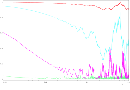
FIG. 1.: Survival probability for different values of $\xi$ ($\xi=1/10,1/3,1,3$ from top to bottom), as functions of $x=\frac{L}{2ER^{2}}$.

The main goal of the next section is to study the mathematical properties of the survival probability and then to compare with experimental data.

B Behavior of survival amplitude and probability

We give here a succinct description of the survival amplitude and probability. Our main goal is to understand their behavior at large $x$, i.e., at large $L/E$ ratio.

We first discuss the eigenvalues of Eq. (2). They can be approached as follows by developing the cotangent:

$$\lambda_{0}\approx \frac{\xi}{\sqrt{1+\frac{\pi^{2}\xi^{2}}{3}}},$$ (8)

$$\lambda_{n}\approx n+\frac{\xi^{2}}{n}+\left(\frac{\pi^{2}\xi^{2}}{3}+1\right)\frac{\xi^{4}}{n^{3}}, {\rm for\,}n\gg\xi^{2},$$ (9)

$$\lambda_{n}\approx n+\frac{1}{2}+\frac{n+\frac{1}{2}}{1+\pi^{2}\xi^{2}}-\frac{\pi^{2}\xi^{4}}{\left(1+\pi^{2}\xi^{2}\right)^{4}}\left(n+\frac{1}{2}\right)^{3}, {\rm for\,}n\ll\xi^{2}.$$ (10)

Their squares $\lambda_{n}^{2}$ give the frequencies appearing in Eq. (5). For $n\gg\xi^{2}$, the first correction to $\lambda_{n}^{2}$ is $2\xi^{2}$, which is an irrelevant global phase. This suggests a strong harmonic behavior of the survival probability, which would justify the use of the approximation $\lambda_{n}\approx n$. Figure 2 shows however that this approximation is very bad indeed when the oscillation regime is entered and that the exact values of $\lambda_{n}$ should be used.

The envelop of the modal amplitudes (4) is a Lorentzian centered at $\lambda=0$ and of width $\xi\sqrt{1+\pi^{2}\xi^{2}}$. For $\xi\ll 1/\pi$, the width is nearly $\xi$; for $\xi\gg 1/\pi$, it approaches $\pi\xi^{2}$. As the Lorentzian falls down rapidly, the width indicates the number of relevant modes according to $\xi$. For numerical calculations, we have checked that it is safe to cut the infinite sum in Eq. (5) after a few widths. Actually at small $\xi$, this means one could even retain only the mode $n=1$.

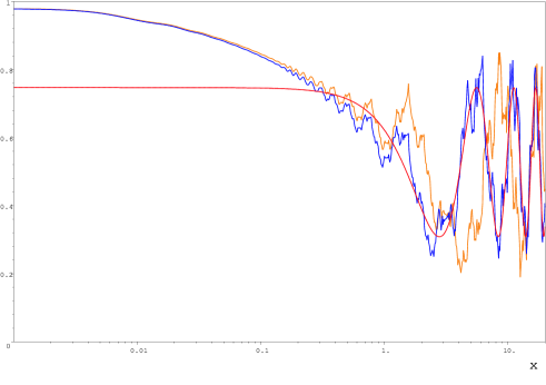
FIG. 2.: Comparison of the survival probability computed using the exact eigenvalues or the approximation $\lambda_{n}=n$ (highest curve to the left) for $\xi=1/3$. For small $x$, the exact survival probability gives lower values, while for $x>1$, the $L/E$ dependence can be completely inverted. The result including only the first oscillatory term is also shown (lowest curve to the left).

From Eq. (6) it is straightforward that the mean value of the survival probability and the amplitude of its fluctuations are given by

$$\left<P_{\nu_{1}\nu_{1}}\right> = \sum_{n=0}^{\infty}\left(U_{0n}\right)^{4},$$ (11)

$$\sigma^{2}\left(P\right) = \left(\sum_{n=0}^{\infty}\left(U_{0n}\right)^{4}\right)^{2}-\sum_{n=0}^{\infty}\left(U_{0n}\right)^{8}.$$ (12)

These results are obtained without any approximation. The mean value $\left<P_{\nu_{1}\nu_{1}}\right>$ is dominated by the zero-mode contribution $\left(U_{00}\right)^{4}$ for $\xi\leq 1/3$, while the large $\xi$ regime, $\left<P_{\nu_{1}\nu_{1}}\right>=\frac{1}{\pi^{2}\xi^{2}}$ is entered from $\xi\approx 0.8$. At large $\xi$, the amplitude of the fluctuations $\sigma\left(P\right)$ tends asymptotically to $\left<P_{\nu_{1}\nu_{1}}\right>$ (see Fig. 3).

It is worth noting another interpretation of this result. Indeed, if we suppose instead that the phases in (5) are uncorrelated, i.e., random frequencies, and perform an average on a set of phase values, we recover the expressions (11,12). This means the frequencies in Eq. (5), although quasiharmonic, do not impose a periodic behavior to the survival probability, especially at large $\xi$. The only harmonic leftover consists in very narrow (and thus phenomenologically irrelevant) periodic peaks in $\left<P_{\nu_{1}\nu_{1}}\right>$.

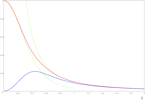
FIG. 3.: Mean survival probability $\left<P_{\nu_{1}\nu_{1}}\right>$ and fluctuations $\sigma(P)$ as functions of $\xi$. The dashed lines give the small $\xi$ ($\left<P_{\nu_{1}\nu_{1}}\right>\approx(U_{00})^{4})$, and the large $\xi$ ($\left<P_{\nu_{1}\nu_{1}}\right>\approx\frac{1}{\pi^{2}\xi^{2}}$) approximations.

Briefly, at large $x$, the survival probability $\left<P_{\nu_{1}\nu_{1}}\right>$ has two regimes.

For small $\xi$, the result is dominated by a constant $\left(U_{00}\right)^{4}$, to which an oscillatory term of frequency $\left(\lambda_{1}^{2}-\lambda_{0}^{2}\right)\approx 1$ is added.

At large $\xi$, the survival probability drops quickly to reach its large $x$ regime: a high frequency fluctuation around its mean value $\frac{1}{\pi^{2}\xi^{2}}$. From a physical point of view, in both cases it is safe to average the survival probability to its mean value if the size of the detector or the source is large (typically $\Delta x\gg 1$). The shape of the survival probability for typical values of $\xi$ is shown on Fig. 1.

C Experimental constraints

We try here to summarize the main experimental results for the survival probabilities $P_{\nu_{e}\nu_{e}}$ and $P_{\nu_{\mu}\nu_{\mu}}$. For $\nu_{e}$ we discuss the CHOOZ experiment, the solar, and the atmospheric neutrinos; for $\nu_{\mu}$, the KARMEN and LSND experiments, the K2K experiment, and the atmospheric neutrinos.

We first discuss the constraints on $P_{\nu_{e}\nu_{e}}$. The CHOOZ experiment[10] gives a very clear and strong constraint on $P_{\nu_{e}\nu_{e}}$. Clear, because the $L/E$ ratio spans less than one order of magnitude. Strong, because the $L/E$ ratio is large (actually larger than for the K2K experiment) and the experiment does not observe any suppression with high precision: $P_{\nu_{e}\nu_{e}}>0.95$, at 90% C.L.

The solar neutrinos are observed by many experiments. We list the observed fluxesin Table I.

TABLE I.: Observed fluxes of the solar neutrinos.

Experiment	Observed to expected	Experimental	Theoretical
	flux ratio	errors	uncertainty (within SSM)
SuperKamiokande [11]	0.47	$\pm$ 0.02	+0.09 / -0.07
Gallex/GNO/Sage[12]	0.60	$\pm$ 0.06	+0.04 / -0.03
Homestake [13]	0.33	$\pm$ 0.03	+0.05 / -0.04

The expected fluxes and theoretical uncertainties are taken from the 1998 Bahcall-Basu-Pinsonneault (BBP98) standard solar model [14] (SSM). The highest experimental precision is reached by SuperKamiokande[11]. We however stress that a sizable uncertainty still lies in the nuclear cross section[15] of the reaction ${}^{7}{\rm Be}+p\rightarrow\;^{8}\!{\rm B}+\gamma$, resulting in a 20% uncertainty in SuperKamiokande. Therefore, the gallium experiments and SuperKamiokande together could be accounted for by a global suppression (neutrino disappearance of 40 to 60%, within the SSM uncertainty). Homestake has a lower value, but is in addition sensitive to the Be lines, for which direct information will only be provided by the upcoming SNO and Borexino experiments.

SuperKamiokande searched for but did not observe any other effect at its current sensitivity: no spectral distortion, no seasonal effect, no day-night effect. A global, energy and distance independent suppression is thus not an unreasonable explanation of the observed solar neutrino deficits.

The atmospheric $\nu_{e}$ flux, observed by SuperKamiokande[17], does not show any distance or energy dependent suppression. The observed angular and energy dependence agrees with the expected one. The main uncertainty here lies in the absolute flux expectation. It turns out that at most 20 to 30% average suppression, without angular or energy dependence, is allowed by the combination of data and Monte Carlo calculations [18].

More robust is the value of the double ratio

$$R=\frac{\left(\nu_{\mu}/\nu_{e}\right)_{\rm observed}}{\left(\nu_{\mu}/\nu_{e}\right)_{\rm expected}}\approx\frac{2}{3}.$$

We now turn to the discussion of the constraints on $P_{\nu_{\mu}\nu_{\mu}}$. The K2K experiment will soon give a constraint on $P_{\nu_{\mu}\nu_{\mu}}$ almost as clean and strong as what CHOOZ obtained for the $\nu_{e}$ survival probability. The $L/E$ ratio also spans less than one order of magnitude. The last available information [19] quotes the following result: 27 observed events, 40$\pm$5 expected.

The atmospheric $\nu_{\mu}$ flux, observed in detail by SuperKamiokande, shows a strong angular and energy dependent suppression. The observed flux, plotted against $L/E$, shows a decrease from $P=1$ to $P=\sim 0.6$, where it levels off. These values are tainted by large errors and are not corrected to take into account initial flux uncertainties (which could be judged from the $\nu_{e}$’s), and thus an extra overall suppression of 20 to 30% is not excluded. Note that the $L/E$ ratio, similar for the $\nu_{e}$’s and $\nu_{\mu}$’s, spans many orders of magnitude, and therefore provides a strong constraint, as we will see in the next subsection.

The KARMEN experiment [20] quotes negative results, i.e., it does not see any $\bar{\nu}_{\mu}$ transition to $\bar{\nu}_{e}$ at small $L/E$ ratio. An upper limit of $6.5\times 10^{-4}$ is put on the transition probability. On the contrary, the LSND experiment [21] claims a 0.3% transition probability $P_{\nu_{e}\nu_{\mu}}$.

D Comparison with experimental data

How can these data be accounted for by the simplest model (one $\nu_{L}$, one KK tower)?

For $\nu_{e}$, we are looking here for possible across the board suppressions at large $x$ by a factor of 40 to 60%, such a solution is the simplest interpretation of the absence of $L/E$ dependence in the SuperKamiokande solar neutrinos data. To prevent any $L/E$ dependence, we should also avoid MSW effects in the Sun or Earth.

As the Sun-Earth system is a very long-baseline system and as the solar core is large (typically, $x\sim 10^{5}$ and $\Delta x\sim 10^{2}\gg 1$ for solar neutrinos with $E\sim 1$ MeV and $R\sim 1$ mm), the only observable effect will be an average suppression. If we fix the suppression range from 40 to 60%, i.e., the mean value $\left<P_{\nu_{e}\nu_{e}}\right>$ at large $x$, we have to take $0.29<\xi<0.42$ approximately. At fixed $\xi$, we then extract the largest allowed $x$ position for CHOOZ still fitting the data. As $L/E$ is known for CHOOZ, this is nothing but an upper limit for $1/R^{2}$.

As $1/R^{2}$ never exceeds $10^{-5}{\rm eV}^{2}$, we always lie in the MSW mass range. The absence of MSW free solution is clearly depicted in Fig. 4. A fit to the solar neutrino problem including the MSW effect has first been proposed in [5]. It needs a very small coupling constant $\xi\sim 10^{-3}$ and gives an energy dependent suppression which can fit the SuperKamiokande results only due to the limited energy resolution of the detector.

We look however for a more drastic, energy independent suppression, which thus needs to avoid MSW effects. This could be reached in two ways. The first consists in increasing the mass of the neutrinos by a constant number, so as to exceed the MSW threshold. Such an approach could be investigated along the lines of [6] but will not be pursued here. Another possibility consists in extending our model to two active neutrinos coupled to one KK tower.

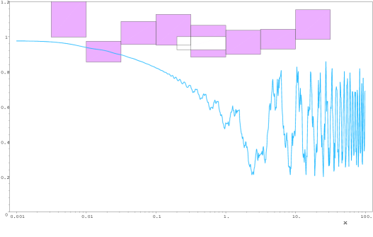
FIG. 4.: Comparison of the toy model with the $\nu_{e}$ constraints. The mean survival probability at large $x$ is fixed at 50% to fit the solar neutrinos. We have plotted the latest available experimental data we could find. The series of filled boxes show the $L/E$ dependence for the atmospheric $\nu_{e}$, as observed by SuperKamiokande (1$\sigma$). The data has been normalized by an overall 0.95 factor with respect to the raw data (instead of the usual $\sim$ 0.9 used by SuperKamiokande). The open box corresponds to the CHOOZ constraint. The error bar at $2\sigma$ level combines quadratically the statistical and systematic errors (see [10]). The boxes cannot slide to the left without getting into the range of the MSW effect, showing thus a complete disagreement with the toy model.

One could also ask whether it would be possible to fit the $\nu_{\mu}$ constraints in the toy model (that is $\nu_{1}=\nu_{\mu}$). Figure 5 shows that a good agreement with the experimental data can be obtained for $\xi=0.4$.

Thus far, we have dealt only for atmospheric neutrinos with the vacuum propagation, neglecting the Earth density effect. This is correct for low energy neutrinos (say, less than 5 GeV for a $\delta m^{2}$ of $10^{-3}{\rm eV}^{2}$), but must be revised for high energy particles where the resulting effective potential becomes determinant. In fact, this is the main reason why sterile neutrinos are now disfavored by the SuperKamiokande experiment in the usual (purely four-dimensional) case [22]. Namely, while a small $\delta m^{2}$ guarantees the desired oscillations and large mixing angle in vacuum, the large effective mass difference between $\nu_{s}$ and $\nu_{e}$ or $\nu_{\mu}$ due to the Earth’s presence lifts the near degeneracy and in practice blocks the oscillations when the density is sufficient. In the four-dimensional case, this occurs for both $\nu$’s and $\bar{\nu}$’s, and results in a contradiction with high energy data (upward through-going muons and partially contained events). Another but rather weaker constraint comes from the multiring, NC enriched sample.

What is the situation in the extra-dimensional case?

We differ from the standard case by the presence of a tower of states. This means that, whatever the density, high energy $\bar{\nu}$’s will always find a state to oscillate to. The effect will thus be at most 1/2 of that expected in the standard situation, with little suppression in the $\nu$’s and large suppression in the $\bar{\nu}$’s. We are thus confident that no serious contradiction occurs.

A detailed simulation of the Earth and angular acceptances is beyond the scope of this paper and will be attempted when we have explored further the full parameter space (which may include additional mass terms for the bulk and/or brane fermions [23]).

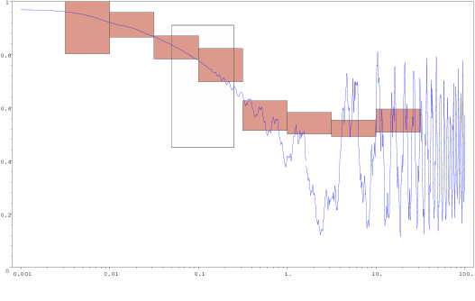
FIG. 5.: Comparison of the toy model with the $\nu_{\mu}$ constraints ($\xi=4/10$). The series of filled boxes show the $L/E$ dependence for the atmospheric $\nu_{\mu}$, as observed by SuperKamiokande (1$\sigma$; the same 0.95 factor has been used). The open box corresponds to the K2K constraint. The error bar at $1\sigma$ level combines quadratically the statistical and systematic errors. The survival probability is in good agreement with the constraints, once an average on each energy ”bin” is performed.

III Two neutrinos coupled to one bulk fermion: the 2-1 model

A Formalism

To solve the solar neutrino puzzle, we now extend the toy model to include a second neutrino in four-dimensional space. We will call $\nu_{e}$ and $\nu_{f}$ the two neutrinos states living in 4 dimensions (we will later discuss the possibility $\nu_{f}=\nu_{\mu}$). The coupling of the flavor neutrinos to the bulk neutrino is chosen in a particularly economical way, the Lagrangian being

$${\cal L}=\lambda_{e}\overline{\nu}_{e}\Psi(x^{\mu},y=0)H(x^{\mu})+\lambda_{f}\overline{\nu}_{f}\Psi(x^{\mu},y=0)H(x^{\mu}).$$ (13)

Therefore, from the four-dimensional point of view, only one linear combination of the two flavor neutrinos, which we call as previously $\nu_{1}$, will be coupled to the Kaluza-Klein tower associated with the bulk fermion $\Psi$. Namely,

$$\nu_{1} = \cos\theta\;\nu_{e}+\sin\theta\;\nu_{f},$$ (14)

$$\nu_{2} = -\sin\theta\;\nu_{e}+\cos\theta\;\nu_{f},$$ (15)

with $\cos\theta=\frac{m_{e}}{m}$ , $\sin\theta=\frac{m_{f}}{m}$, $m=\sqrt{m_{e}^{2}+m_{f}^{2}}$ and $m_{e,f}=\frac{\lambda_{e,f}v}{\sqrt{2\pi R}}$ . The orthogonal combination $\nu_{2}$ remains massless.While the mixing with bulk states proceeds exactly as before, the physical consequences can be quite different. Indeed, a new phenomenological parameter, the mixing angle $\theta$ now plays a crucial role in the survival probabilities of the flavor neutrinos,

$$P_{\nu_{e}\nu_{e}} = \cos^{4}\theta\;P_{\nu_{1}\nu_{1}}+\sin^{4}\theta+2\sin^{2}\theta\;\cos^{2}\theta\;\textrm{Re}\left(A_{\nu_{1}\nu_{1}}\right),$$ (16)

$$P_{\nu_{f}\nu_{f}} = \sin^{4}\theta\;P_{\nu_{1}\nu_{1}}+\cos^{4}\theta+2\sin^{2}\theta\;\cos^{2}\theta\;\textrm{Re}\left(A_{\nu_{1}\nu_{1}}\right).$$ (17)

The flavor transition probability is given by

$$P_{\nu_{e}\nu_{f}}=P_{\nu_{f}\nu_{e}}=\sin^{2}\theta\ \cos^{2}\theta\ \left[P_{\nu_{1}\nu_{1}}-2\textrm{Re}\left(A_{\nu_{1}\nu_{1}}\right)+1\right].$$ (18)

This model (hereafter called the 2-1 model) has 3 degrees of freedom, $(\xi,\theta,R)$, to fit the experimental data which also include the different bounds to the $\nu_{\mu}(\overline{\nu}_{\mu})$ fluxes, in case $\nu_{f}=\nu_{\mu}$ is chosen. We should also stress that $\theta$ is not the $\nu_{e}-\nu_{f}$ mixing angle. Such mixing arises, but only as a result of the independent coupling of both states to the bulk neutrino.

B Comparison with experimental data

In the first part of this analysis, we will concentrate on the electronic neutrino data. We will show that, taking advantage of the second active neutrino, we can now fit all the experimental constraints on the electronic neutrino without getting into the MSW region.

The solar neutrino deficit is accounted for if the $\nu_{e}$ mean survival probability at large $x$ ranges between 40% to 60% max. as a result of the experimental and SSM uncertainties. This constraint defines a region in the plane $\xi-\theta$ as shown in Fig. 6.

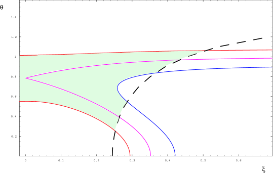
FIG. 6.: Region of values for $\xi$ and $\theta$ for which the solar and CHOOZ constraints for $\nu_{e}$ can be accommodated without MSW effect. The solid lines correspond (from top to bottom) to a solar neutrino mean survival probability of 60, 50, and 40%. The dashed line indicates the frontier of the MSW region in view of the CHOOZ constraint. The filled region gives the allowed $(\xi,\theta)$ values.

For small values of $\theta$, $\nu_{e}$ is mainly $\nu_{1}$ , so that the allowed values of $\xi$ range from 0.3 to 0.42. For higher values of $\xi$ indeed, the electronic neutrino survival probability drops under 40%, while for lower values, it does not decrease below 60%. As the mixing angle $\theta$ increases, the proportion of the decaying component of $\nu_{1}$ diminishes, so that the allowed range for $\xi$ gets enlarged. Finally, if $\theta$ is too big ($1<\theta<\pi/2$ approximately), the decaying component of $\nu_{e}$ is insufficient to explain the solar neutrino deficit.

The next constraint comes from the CHOOZ nuclear reactor experiment. As seen before, the $\overline{\nu}_{e}$ produced in the reactor with a typical energy of 2 MeV show no disappearance at a distance $L=1~{}$ km.

For given $\xi$ and $\theta$, a maximum admissible value of $x$, or equivalently, a minimum value of $R$ (the radius of the compactified extra dimension) results. The value of $x$ increases with $\theta$ at given $\xi$, but decreases with $\xi$ at fixed $\theta$ . Therefore, a small coupling constant $\xi$ and a large mixing angle $\theta$ are preferred in view of the CHOOZ experiment.

On the other hand, $1/R$ controls the typical mass difference between two consecutive Kaluza-Klein levels. Therefore, MSW resonant conversion will take place if $1/R$ is of the same magnitude order as the MSW potential. As suggested by the latest SuperKamiokande data, we can put an upper bound on $R$ and avoid the MSW effect. Typically, $R_{\max}\simeq 10^{-2}$ mm. As a result, for some $\xi$ and $\theta$, this bound can be incompatible with the CHOOZ constraint. This is shown in Fig. 6. The constraint arising from the unsuppressed flux of the atmospheric $\nu_{e}$ will be discussed later, as it depends on the flavor of the second active neutrino. We can already announce that it favors the case $\nu_{f}=\nu_{\mu}$, yet the case $\nu_{f}=\nu_{\tau}$ remains also possible. Therefore, all constraints on $P_{\nu_{e}\nu_{e}}$ can be satisfied in the 2-1 model. It is also clear that a nonzero mixing angle $\theta>0$ is needed.

We now study in detail the possibility $\nu_{f}=\nu_{\mu}$. We first discuss the $\overline{\nu}_{\mu}$ disappearance experiment K2K, which reveals some 30% deficit for 2 GeV neutrinos at a distance $L\simeq 250$ km. We have $x_{\rm K2K}\simeq 1/4\cdot x_{\rm CHOOZ}$, so that muonic neutrinos are expected to disappear more than electronic neutrinos. This requires $\theta>\pi/4$, and higher values of $\xi$ are favored, as $P_{\nu_{e}\nu_{e}}-P_{\nu_{\mu}\nu_{\mu}}\propto(1-P_{\nu_{1}\nu_{1}})$. However, even for the maximal allowed $\xi$, the preliminary result of K2K can only be accommodated by taking the large statistical error into account. Figure 7 shows a possible fit for $\nu_{e}$ and $\nu_{\mu}$, which solves the solar neutrino problem, and simultaneously satisfies the CHOOZ and K2K constraints. It will be shown hereafter that this fit also satisfies the constraints for the atmospheric neutrinos.

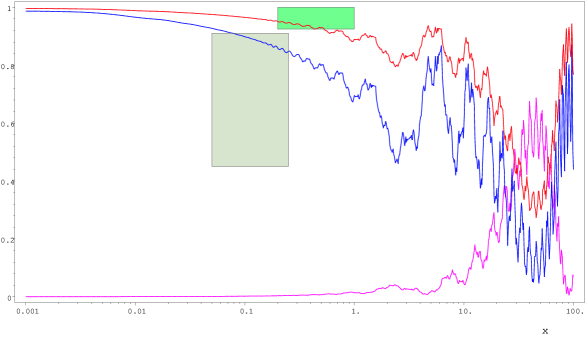
FIG. 7.: Comparison of the 2-1 model with the CHOOZ and K2K constraints. (highest curve is for $\nu_{e}$) $\xi=0.3$ and $\theta=1.05$, so that $\left<P_{\nu_{e}\nu_{e}}\right>\simeq 60\%$. The transition probability $P_{\nu_{e}\nu_{\mu}}$ is also depicted (lowest curve).

To discuss the constraints coming from the atmospheric neutrinos, we recall that in the 2-1 model, a transition $\nu_{e}\rightarrow\nu_{\mu}$ or $\nu_{\mu}\rightarrow\nu_{e}$ becomes possible. The transition probability, as shown in Fig. 7, is non-negligible in the range of the atmospheric neutrinos. As the atmospheric neutrinos originate from the decay of the charged pions and kaons into muons and the subsequent decay of muons into electrons, the ratio of the neutrino initial fluxes $\frac{\phi^{(i)}_{\nu_{\mu}}}{\phi^{(i)}_{\nu_{e}}}$ is expected to be very close to 2, especially at low energy. Therefore, the expected neutrino flux in the 2-1 model with $\nu_{f}=\nu_{\mu}$ is given by (we do not distinguish between $\nu$ and $\overline{\nu}$)

$$\frac{\phi_{\nu_{e}}}{\phi^{(i)}_{\nu_{e}}}=P_{\nu_{e}\nu_{e}}+2\,P_{\nu_{\mu}\nu_{e}}$$ (19)

$$\frac{\phi_{\nu_{\mu}}}{\phi^{(i)}_{\nu_{\mu}}}=P_{\nu_{\mu}\nu_{\mu}}+1/2\,P_{\nu_{e}\nu_{\mu}},$$ (20)

As a result, the observed $\nu_{e}$ flux can be enhanced compared to the initial production flux in our model. In Fig. 8, we see that this picture is in very good agreement with the SuperKamiokande results.

We are left with the constraints of KARMEN and LSND. The negative result of the KARMEN experiment can easily be accommodated as $x_{\rm KARMEN}\simeq 3\times 10^{-4}\ x_{\rm CHOOZ}$. On the contrary, as $x_{\rm LSND}\simeq 6\times 10^{-4}\ x_{\rm CHOOZ}$, our model can never comply with the LSND results, for any allowed values of $\theta$ and $\xi$.

We have thus shown that all experimental data (with the exception of LSND) can be accommodated in the simple 2-1 model with $\nu_{f}=\nu_{\mu}$,that is with $\nu_{e}$ and $\nu_{\mu}$ coupled to the same Kaluza-Klein tower. However the fit could be invalidated in the near future should the LSND signal be confirmed by an independent experiment. A critical test will also be provided by the improving accuracy of the K2K experiment. We also point out that the astrophysical bound could be evaded in this model, since the disappearance of $\nu_{e}$ or $\nu_{\mu}$ in the extra dimensions is never complete (see [24]).

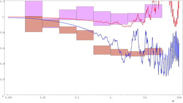
FIG. 8.: Expected atmospheric neutrino fluxes in the 2-1 model with $\nu_{f}=\nu_{\mu}$ and the SuperKamiokande data. $\xi=0.3$ and $\theta=1.05$ as in Fig. 7. The initial flux $2\stackrel{{\scriptstyle(-)}}{{\nu_{\mu}}}+\stackrel{{\scriptstyle(-)}}{{\nu_{e}}}$ is normalized to 1 at $x=0$. The observed SuperKamiokande data has been normalized as in Fig. 4. The agreement with experimental data is quite remarkable.

Can we improve the fit to $\nu_{e}$ data by allowing for $\nu_{f}\neq\nu_{\mu}$ ? For instance, we could have $\nu_{f}=\nu_{\tau}$ or $\nu_{f}=\nu_{s}$, with $\nu_{s}$ an extra four-dimensional sterile neutrino. Of course, the model is no longer affected by $\nu_{\mu}$ observations, but strong constraints like CHOOZ remain, and must be reconciled with solar data, given the allowed region of Fig. 6. The real difficulty could, however, come from the atmospheric $\nu_{e}$. In the ($\nu_{e}-\nu_{\mu}-KK$) model indeed, the atmospheric $\nu_{e}$ flux at long distance was boosted by a $\nu_{\mu}\rightarrow\nu_{e}$ conversion. Here, with the $\nu_{e}$ and $\nu_{\mu}$ sectors separated, boosting disappears, and the $\nu_{e}$ flux falls more rapidly. Still, given the uncertainty on the absolute normalization of the atmospheric $\nu_{e}$, no contradiction exists for the moment. Actually, the constraint provided by the CHOOZ experiment appears to be more severe, so that the allowed region of parameters that give a good fit to the $\nu_{e}$ data is still given by Fig. 6.

We have also checked that a ($\nu_{e}-\nu_{\mu}-\nu_{\tau}-KK$) approach along the present lines does not improve the quality of the fit.

IV Conclusions

We have shown that a simple model with 2 massless neutrinos coupled to one Kaluza-Klein tower meets most experimental constraints (except for LSND), and differs from the oscillation image by the energy dependence of the neutrino disappearance. This model can be developed by adding extra parameters in the form of bare masses for the neutrinos, while simply increasing the number of neutrinos coupled to the Kaluza-Klein states brings little gain.

REFERENCES

- [1] N. Arkani-Hamed, S. Dimopoulos and G. Dvali, Phys. Lett. B 429 (1998) 263.
- [2] I. Antoniadis, N. Arkani-Hamed, S. Dimopoulos and G. Dvali, Phys. Lett. B 436 (1998) 257.
- [3] N. Arkani-Hamed, S. Dimopoulos, G. Dvali and J. March-Russell, hep-ph/9811448.
- [4] K. R. Dienes, E. Dudas, T. Gherghetta, Nucl. Phys. B 557 (1999) 25.
- [5] G. Dvali and A. Y. Smirnov, Nucl. Phys. B 563 (1999) 63.
- [6] A. Lukas, P. Ramond, A. Romanino and G. G. Ross, Phys. Lett. B 495 (2000) 136.
- [7] A. Pérez-Lorenzana, hep-ph/0008333; lectures given at the IX Mexican School on Particles and Fields, Metepec, Puebla, Mexico, August, 2000.
- [8] R. Barbieri, P. Creminelli and A. Strumia, Nucl. Phys. B 585 (2000) 28.
- [9] R. N. Mohapatra and A. Pérez-Lorenzana, Nucl. Phys. B 593 (2001) 451.
- [10] M. Apollonio et al. [CHOOZ Collaboration], Phys. Lett. B 466 (1999) 415.
- [11] Y. Suzuki [Super-Kamiokande Collaboration], Nucl. Phys. Proc. Suppl. 77 (1999) 35; Y. Suzuki, talk transparencies at Neutrino2000 (http://nu2000.sno.laurentian.ca/); Y. Takeuchi, talk transparencies at Ichep2000 (http://ichep2000.hep.sci.osaka-u.ac.jp/).
- [12] P. Anselmann et al. [GALLEX Collaboration], Nucl. Phys. Proc. Suppl. 38 (1995) 68; M. Altmann et al. [GNO Collaboration], Phys. Lett. B 490 (2000) 16; C. Cattadori, talk transparencies at Ichep2000 (http://ichep2000.hep.sci.osaka-u.ac.jp/); J. N. Abdurashitov et al. [SAGE Collaboration], Phys. Atom. Nucl. 63 (2000) 943 [Yad. Fiz. 63 (2000) 1019].
- [13] B. T. Cleveland et al. [Homestake Collaboration], Nucl. Phys. Proc. Suppl. 38 (1995) 47.
- [14] J. N. Bahcall, S. Basu and M. H. Pinsonneault, Phys. Lett. B 433 (1998) 1.
- [15] E. G. Adelberger et al., Rev. Mod. Phys. 70 (1998) 1265; F. Hammache et al., Phys. Rev. Lett. 80 (1998) 928.
- [16] R. Escribano, J. M. Frère, A. Gevaert and D. Monderen, Phys. Lett. B 444 (1998) 397; J. N. Bahcall and P. I. Krastev, Phys. Lett. B 436 (1998) 243; see also [11].
- [17] J. G. Learned [SuperKamioKande Collaboration], hep-ex/0007056, Chapter in Current Aspects of Neutrino Physics; H. Sobel, talk transparencies at Neutrino2000 (http://nu2000.sno.laurentian.ca/); T. Toshito, talk transparencies at Ichep2000 (http://ichep2000.hep.sci.osaka-u.ac.jp/); M. D. Mesier, Ph.D. thesis, available at http://www-sk.icrr.u-tokyo.ac.jp/doc/sk/pub.
- [18] HONDA Model, M. Honda, T. Kajita, K. Kasahara and S. Midorikawa, Phys. Rev. D 52 (1995) 4985; BARTOL Model, G. Barr, T. K. Gaisser and T. Stanev, Phys. Rev. D 39 (1989) 3532; V. Agrawal, T. K. Gaisser, P. Lipari and T. Stanev, Phys. Rev. D 53 (1996) 1314; 3D FLUKA Model, G. Battistoni et al., Astropart. Phys. 12 (2000) 315; P. Lipari, Astropart. Phys. 14 (2000) 153; P. Lipari, Astropart. Phys. 14 (2000) 171.
- [19] K. Nakamura, talk transparencies at Neutrino2000 (http://nu2000.sno.laurentian.ca/); M. Sakuda, talk transparencies at Ichep2000 (http://ichep2000.hep.sci.osaka-u.ac.jp/).
- [20] J. Kleinfeller [KARMEN Collaboration], Nucl. Phys. Proc. Suppl. 87 (2000) 281; K. Eitel [KARMEN Collaboration], Nucl. Phys. Proc. Suppl. 91 (2000) 191.
- [21] E. D. Church [LSND Collaboration], Nucl. Phys. A 663 (2000) 799; G. Mills, talk transparencies at Neutrino2000 (http://nu2000.sno.laurentian.ca/).
- [22] S. Fukuda et al. [Super-Kamiokande Collaboration], Phys. Rev. Lett. 85 (2000) 3999.
- [23] A. Lukas, P. Ramond, A. Romanino and G. G. Ross, hep-ph/0011295.
- [24] K. R. Dienes and I. Sarcevic, Phys. Lett. B 500 (2001) 133.