1

HOT OR DENSE MATTER

PETER ARNOLD

Department of Physics, University of Virignia, P.O. Box 400714

Charlottesville, Virginia 22904-4714, USA

I review some of the properties of hot and/or dense relativistic matter.

I’ve been asked to review hot and/or dense matter. As a general rule, most particle physicists aren’t that familiar with the behavior of quantum field theory at finite temperature and density. We’ve all been introduced to how to think about systems of a few relativistic particles with given energies, and how to describe such systems with quantum field theory, but most of us haven’t had occasion to develop comparable experience and intuition about systems of many particles at finite temperature or density. I am therefore going to forgo attempting a comprehensive review of recent results. Instead, I will try to give a primer on relativistic hot or dense matter, with a perhaps somewhat quirky choice of topics dictated by my own areas of competence.

To begin, let me define some terms. Matter will mean gauge theories (coupled to fermions and so forth). As far as gauge theories go, I’ll restrict my attention to QCD and electroweak theory. Hot or dense will mean relativistically, and even ultra-relativistically, hot or dense.

Ultra-relativistically hot QCD matter is matter at high density: if there weren’t any initially, they’d instantly appear due to pair creating collisions of photons or gluons or whatever. However, in this field, the adjective “dense” is used instead as a codeword to mean “non-zero chemical potential $\mu$.” More specifically, dense typically refers to non-zero chemical potential $\mu_{\rm B}$ for baryon number. So dense QCD refers to the case where the numbers of quarks and anti-quarks are significantly different.

1 Hot Matter

I’ll begin by focusing just on hot matter, by which I mean $\mu=0$ or close to it ($\mu\ll T$). This is the situation of relevance to the early Universe at temperatures above the QCD scale, when the asymmetry between the number of quarks and anti-quarks was very small.

1.1 Example: Electroweak baryogenesis

One example of a situation where the physics of hot (but not “dense”) gauge theories is of interest is electroweak baryogenesis.^? Electroweak baryogenesis is an attempt to explain the current dominance of matter over anti-matter in our Universe in terms of electroweak physics. It is based on the theoretical prediction that the standard model violates baryon number at temperatures larger than the electroweak scale. This is a non-perturbative feature of the standard model, and it is caused by certain types of non-perturbative fluctuations of electroweak gauge fields. Specifically, the change in baryon number $B$ turns out to be related to the behavior of the electroweak gauge fields by what’s known as an anomaly equation:

$$\Delta B=\#g_{\rm w}^{2}\int d^{4}x\>{\rm tr}\,F_{\rm w}\tilde{F}_{\rm w}.$$ (1)

I’m not actually going to need this equation for anything—just remember that hot electroweak $B$ violation requires non-perturbatively large fluctuations in the gauge fields.

It turns out that the probability of such non-perturbative fluctuations is exponentially sensitive to the mass of the W and so is exponentially sensitive to the expectation value $\langle\phi\rangle$ of whatever plays the role of the Higgs, since that’s where the W’s mass comes from. At the present time, with $\langle\phi\rangle$ of order the weak scale, the rate for electroweak baryon number violation is predicted to be so tiny that you wouldn’t see it even if your proton decay experiment was the size of the observable universe and ran for 15 billion years. However, in the very early universe, $\langle\phi\rangle$ was effectively zero, and $B$ violation is predicted to have been large. Depending on the details of the Higgs sector, there could have been an abrupt, supercooled, first-order phase transition between the original, hot, symmetry-restored ($\langle\phi\rangle=0$) phase of electroweak theory and the current symmetry-broken phase ($\langle\phi\rangle\not=0$). This transition is the focal point of scenarios of electroweak baryogenesis, a cartoon for which is shown in Fig. 1. A supercooled first-order transition would proceed by the nucleation and expansion of bubbles of the symmetry-broken phase. Such a bubble is shown in Fig. 1a. As the bubble expands, it will run into quarks and anti-quarks present in the hot plasma that filled the Universe at that time. Because of CP violating interactions with the bubble wall, it is possible for quarks to be able to penetrate the bubble wall slightly more often than anti-quarks. This results in an anti-quark excess building up in a shell outside the wall (and a quark excess inside) as depicted in Fig. 1b. Baryon number violation processes in that shell attempt to locally restore chemical equilibrium by converting those excess anti-quarks into quarks, and so increasing the baryon number of the Universe. There is no balancing conversion of the excess quarks inside the bubble wall because $B$ violation is not significant in the symmetry-broken phase, as I asserted earlier. So, in net, a baryon number $B>0$ for the universe is generated.

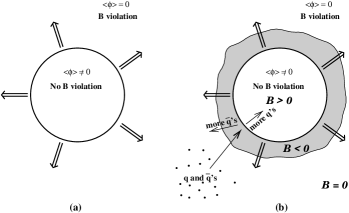
Figure 1: A cartoon of electroweak baryogenesis.

This scenario generates all sorts of interesting theoretical problems to work on. For example, one would like to know how to compute the rate of non-perturbative processes, such as $B$ violation, in hot gauge theory. As another example, many aspects of the bubble wall growth depend on hydrodynamics of the quark-gluon-W-Z-etc. plasma. The parameters of hydrodynamics are known as transport coefficients—viscosities, diffusion constants, etc.—and one would like to know how to compute them from first principles.

The rate of $B$ violation is a non-perturbative problem, and the usual way to attack non-perturbative problems from first principles is to make lattice simulations. However, there is a difficulty here: standard lattice methods for quantum field theory are based on simulations in imaginary time, and the quantities of interest here live in real time! This is potentially an extremely serious difficulty, and I’ll discuss later how it is overcome.

1.2 Hot matter at small coupling

The example of electroweak baryogenesis shows that there are interesting questions to be addressed even in weakly-coupled hot field theories, such as hot electroweak theory. And, in studying relativistically hot plasmas more generally, it seems a good idea to try to understand something you might at first think was relatively simple—the weak coupling limit. So, for the rest of my talk, I’ll specialize to very hot QCD and Electroweak theory at small coupling, by which I mean that $g(T)\ll 1$, where $g(T)$ is the running coupling constant at the scale of the temperature $T$. Also, for simplicity (and because it’s plenty complicated enough), I will focus on hot physics in systems that are at or near equilibrium.

1.2.1 Isn’t small coupling trivial?

You might think the small coupling limit is trivial, though possibly tedious, to analyze: you just lock a theorist up in a closet with some paper and have them do perturbation theory by computing a bunch of Feynman diagrams to whatever order is desired. At high temperature, however, small coupling does not mean perturbative. A simple way to understand this is to think not of field theory but simple quantum mechanics. Consider a slightly anharmonic oscillator, depicted in fig. 2, with potential energy of the form

$$V(x)\sim\omega_{0}^{2}x^{2}+g^{2}x^{4},$$ (2)

and suppose that $g^{2}$ is very, very small. In the ground state, the wave function will be localized around $x=0$, and one will be able to treat $g^{2}x^{4}$ as a perturbation compared to $\omega_{0}^{2}x^{2}$. But now consider the state of the system at high temperature. The larger the temperature, the larger the energy, in which case the larger the values of $x$ the system will be able to probe. For large enough $x$, a quartic $g^{2}x^{4}$ will always dominate over a quadratic $\omega_{0}^{2}x^{2}$, and so $g^{2}x^{4}$ cannot be treated as a perturbation to $\omega_{0}^{2}x^{2}$.

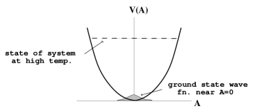
Figure 2: A slightly anharmonic oscillator.

The physics of the slightly anharmonic oscillator becomes non-perturbative at large $T$, but it also becomes classical. The state of the system corresponds to very high level numbers, and so is classical by the correspondence principle. This is important: As I’ll discuss later, it is the classical nature of the non-perturbative physics that makes it possible to do real-time lattice simulations for hot gauge theories.

Now note that if we fixed $T$ but varied $\omega_{0}$, and took $\omega_{0}\to 0$, we’d again get to a non-perturbative situation where $g^{2}x^{4}$ cannot be treated perturbatively compared to $\omega_{0}^{2}x^{2}$. This observation allows us to see how this quantum mechanical example translated to field theory. Hot gauge theory can be thought of as coupled QM oscillators corresponding to each Fourier mode ${\bf k}$, with corresponding natural frequencies $\omega_{k}\sim k$. In QM, we see that $\omega_{0}\to 0$ at fixed $T$ leads to non-perturbative physics. In hot gauge theory, $\omega_{k}\sim k\to 0$ will analogously lead to non-perturbative physics. It is therefore the low-momentum (long wavelength) modes of hot gauge theory that have non-perturbative fluctuations at high temperature. It turns out that the momentum scale at which the physics becomes non-perturbative is $k\sim g^{2}T$.

1.2.2 Hey, what about deconfinement?

I’ve asserted that there is non-perturbative physics in very hot gauge theories. You might wonder how this is consistent with the picture that QCD deconfines at high temperature and, because of asymptotic freedom, can be treated as a weakly-interacting gas of quarks and gluons. The origin of deconfinement is something that you learned from Jackson in graduate school: static electric fields are Debye screened in plasmas. For an Abelian theory, the Coulomb potential $g^{2}/r$ between two static test charges is modified by Debye screening to a Yukawa potential $g^{2}e^{-m_{\rm D}T}/r$. In non-Abelian theories, a similar exponential screening of the potential occurs, screening away the linear long-distance potential that is responsible for confinement. In the ultra-relativistic limit, the inverse screening length $m_{\rm D}$ turns out to be of order $gT$.

Static magnetic fields, however, are not screened in plasmas. This is why it’s possible, for instance, for the Sun and the galaxy to have magnetic fields. It is these unscreened magnetic fields which can produce non-perturbative physics.

It’s worth mentioning, for the sake of later discussion, that plasmas do resist dynamical magnetic fields. This is due to what’s known in introductory physics as Lenz’s Law: conductors resist changes in magnetic field. Plasmas are conductors, and changes in the magnetic field create electric fields, which then create currents in the plasma, which create magnetic fields opposing the original change.

I have now introduced you to a hierarchy of momentum scales in weakly coupled ultra-relativistic plasmas:

$T$	energy/momentum of typical particles in the plasma;
$gT$	inverse Debye screening length;
$g^{2}T$	non-perturbative magnetic fluctuations.

Other scales of interest turn out to include the mean free path for color-randomizing collisions, which is order $g^{2}T\ln(1/g)$, and the mean free path for large-angle scattering, which is $g^{4}T\ln(1/g)$. The trick to studying hot physics turns out to be to find and exploit appropriate effective theories which describe the physics at each scale of interest, and systematically match the parameters of those effective theories to the original gauge theory.

1.2.3 Small coupling expansion is NOT the loop expansion

Even though perturbation theory fails at high temperature, there is no reason that one can’t Taylor expand the result for physical quantities in powers of the small coupling $g$. For instance, the free energy of a hot non-Abelian gauge theory has an expansion of the form^?

$$F=T^{4}\left[\#+\#g^{2}+\#g^{3}+\#g^{4}+\#g^{5}\left(\ln{1\over g}+\#\right)+\#g^{6}\left(\ln{1\over g}+\mbox{\bf\hbox to0.0pt{\#\hss}{\kern 1.0pt\#}}\right)+\cdots\right].$$ (3)

Here, the $g^{0}$ term is the ideal gas result, and the other terms are corrections due to interactions. The fact that this is not simply the loop expansion is manifest from the appearance of odd powers of $g$, as well as logs of $1/g$. The terms through $g^{5}$ can in fact be calculated by pencil and paper using appropriately resummations of perturbation theory, but the $g^{6}$ term denoted by the boldface ## is the leading contribution to the free energy from truly non-perturbative magnetic physics. It can’t be calculated with pencil and paper.

We are used to seeing logs of ratios of physical scales in zero temperature results. For instance, the transverse distribution for producing W’s in a collider has logs of $p_{\rm T}/M_{\rm w}$. In the previous section, I discussed how relevant physical scales at finite temperature are $T$, $gT$, and $g^{2}T$. It is logs of the ratios of such scales that produce the logs of $1/g$ in (3). [Ratios of these scales are also responsible for the odd powers of $g$ in (3).]

The free energy is an example where non-perturbative physics doesn’t show up until high order in the small-coupling expansion (which is why it remains useful to think of the plasma as a weakly-interacting gas of quarks and gluons). There are other quantities, such as baryon number violation, that are intrinsically non-perturbative. The baryon number violation rate per unit volume turns out to have a small-coupling expansion of the form^?

$$\Gamma_{\rm B}=\mbox{\bf\hbox to0.0pt{\#\hss}{\kern 1.0pt\#}}g_{w}^{10}T^{4}\left(\ln{1\over g}+\#\right)+\cdots,$$ (4)

where ## is a coefficient that cannot be computer with pencil and paper.

To emphasize the difference between the small coupling expansion and the loop expansion, here’s the small coupling expansion for the inverse of the shear viscosity, which is^?

$$\eta^{-1}=\#g^{4}T^{-3}\ln{1\over g}+\cdots.$$ (5)

Diagrammatically, the leading term comes from an infinite subset of perturbative diagrams, an example of which is shown in fig. 3.

Figure 3: Example of the infinite class of diagrams that contribute to the leading-order result for inverse shear viscosity.

1.3 Effective Theories

Summing up infinite classes of diagrams by hand, such as those suggested by fig. 3, is a pain in the butt, and is also of little use if your ultimate interest is calculating something non-perturbative. The most efficient way to proceed is to instead figure out effective theories of the long-distance physics, which can be matched to the short-distance physics of the original theory.

If one is interested in non-dynamical questions about hot, equilibrium gauge theories—that is, if one doesn’t care about time dependence—then analyzing the system in imaginary time is just as good as analyzing it in real time. The use of effective theories appropriate to imaginary-time analysis has a long history and is well understood and well under control. I won’t dwell on it here, except in a footnote.

Over the past few years, progress has been made in understanding the sequence of effective theories that efficiently describe dynamical questions (baryon number violation, transport coefficients, …) at different scales. As suggested earlier, long distance physics is classical at high temperature. The appropriate effective theory for distance scales large compared to $1/T$ (i.e. momenta small compared to $T$) can be described in classical terms by what is known as a Boltzmann-Vlasov equation. The state of the system at any time is represented by two types of classical functions. The first, $n_{i}({\bf x},{\bf p},t)$, represents the density in phase space of particles of a given type $i$ (specifying flavor, color, and spin) at position ${\bf x}$ carrying momentum ${\bf p}$. The second, $A({\bf x},t)$, represents the configuration of the ${\it long{-}wavelength}$ modes of the gauge fields. (Gauge field quanta with short wave-lengths are treated as particles and incorporated into the $n_{i}$’s.) The equation that describes the time evolution is simply a Boltzmann equation, which describes the effects on the densities $n_{i}$ due to (1) free streaming in the background of the long-wavelength field $A$, and (2) changes in ${\bf p}$ due to collision among each other. Schematically, the equation looks like

$$(D_{t}+{\bf v}\cdot{\bf D})n+g({\bf E}+{\bf v}\times{\bf B})\cdot\mbox{\boldmath$\nabla$}_{\bf p}n=\mbox{collision term}.$$ (6)

The first term is a convective derivative (which tells you that $n$ can change at a given ${\bf x}$ simply because the particles’ momenta carried them away to a different ${\bf x}$) The second term accounts for the force on the particles due to the long wavelength gauge fields. The collision term, if one were to write it out, involves expressions like

$$\int_{234}|{\cal M}_{12\to 34}|^{2}n_{1}n_{2}(1\pm n_{3})(1\pm n_{4}),$$ (7)

where ${\cal M}_{12\to 34}$ is, for example, a $2\to 2$ scattering amplitude, and the $(1\pm n)$’s are final-state Bose enhancement or Fermi blocking factors. Finally, one also needs the equation for the time evolution of the long-wavelength gauge fields, which is just Maxwell’s equation,

$$D_{\mu}F^{\mu\nu}=j^{\nu}=\int_{\bf p}gv^{\mu}\,n({\bf p}),$$ (8)

with sources provided by the particles described by the $n$’s. These two, simple, physically motivated equations reproduce what are known as “hard thermal loops,” which was historically the original analysis of the effective dynamics at long distances, based on a difficult analysis of resumming Feynman diagrams.

At yet larger distance scales, large compared to the scale $g^{4}T\ln(g^{-1})$ which turns out to characterize the mean-free path for large-angle scattering, the appropriate effective theory becomes linearized hydrodynamics. (The Boltzmann-Vlasov effective theory is still valid, but, like the original quantum field theory, is no longer an efficient description for calculations.)

There is an important unresolved issue in the use of effective theories for studying dynamical properties. Unlike the non-dynamical case, it is somewhat unclear how to improve the validity of these effective theories beyond leading order in powers of $g$. (At least, nobody has ever done a systematic calculation of a physical quantity beyond leading order.)

1.4 Example: numerical simulations of the B violation rate

The nice thing about a classical theory is that, in principle, it’s straightforward to simulate it in real time.  You discretize space into a lattice, pick initial configurations from a thermal ensemble, evolve each configuration forward in time using the classical equations of motion, and then measure whatever you wanted to measure. The classical equations discussed previously (as well as some even simpler effective theories I don’t have time to discuss) have been used to simulate the rate of baryon number violation. Doing this a variety of different ways with a variety of variations on the classical effective theory, various subsets of Moore, Bödeker, Rummukainen, Hu, and Müller have found^?

$$\Gamma_{\rm B}\simeq\pmatrix{25\pm 2\cr 25\pm 7\cr 29\pm 6}\alpha_{\rm w}^{5}T^{4}$$ (9)

for the Standard Model with $\alpha_{\rm w}\simeq 1/30$. [I have not explicitly shown the $\ln(1/\alpha_{\rm w})$ factors but have incorporated them into the numbers.]

2 Dense Matter

I’ll now switch to a discussion of dense matter (sometimes also hot, sometimes not) — that is, matter at non-zero chemical potential for baryon number. I should disclose that I am not on expert at this subject, and there were many people at the DPF conference much more knowledgeable than I.

Even non-dynamical questions about dense matter are problematical for lattice simulations. The problem is that the imaginary-time path integral has the form

$$\int[{\cal D}A]\>[{\cal D}\psi][{\cal D}\bar{\psi}]\>\exp[-S_{\rm YM}-\bar{\psi}(\mbox{\hbox to0.0pt{$D$\hss}{\kern 2.0pt/}}+m+i\mu\gamma_{0})\psi]$$

$$\hskip 80.00012pt=\int[{\cal D}A]\>\exp[-S_{\rm YM}]{\det}^{N}(\mbox{\hbox to0.0pt{$D$\hss}{\kern 2.0pt/}}+m+i\mu\gamma_{0}),$$ (10)

and, because of the $i\mu\gamma_{0}$, the integrand on the right-hand side is not positive real. That means that the integrand can’t be interpreted as a probability measure on which to base a Monte Carlo algorithm.

It’s interesting to note that, despite the $i\mu\gamma_{0}$, the determinant does turn out to be positive real for (a) two-color QCD,^? or (b) non-zero isospin chemical potential instead of non-zero baryon number chemical potential.^? These unrealistic cases should provide nice opportunities for numerical simulation to test theoretical attempts to analyze gauge theories at non-zero chemical potential.

2.1 Example: The phase diagram of hot, dense QCD

One educated guess as to what the phase diagram of hot, dense QCD might look like is shown in fig. 4, which I stole from a conference talk of Krishna Rajagopal’s.^? The phases marked 2SC and CFL are color superconducting phases in which a color-breaking diquark condensate $\langle qq\rangle\not=0$ forms. 2SC denotes a 2-flavor (u,d) color superconductor in which the SU(3) color gauge group is only partly broken and in which chiral symmetry is unbroken. CFL (an acronym for Color Flavor Locking) denotes a 3-flavor (u,d,s) color superconductor in which chiral symmetry is broken.

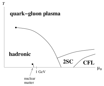
Figure 4: Educated guess at phase diagram of hot and dense QCD.^?

Readers may well be interested to understand what to make of the claims in the press that CERN has already discovered the quark-gluon plasma region of this diagram. Readers might be interested to know what the prospects are for RHIC and the LHC to explore, verify, or falsify any of the features of fig. 4. These are interesting and important questions. They are also complicated and intricate questions. Now recall that earlier in this talk, I said I would focus on gauge theories at weak coupling. So, for the sake of consistency, I sadly but clearly have no choice but to ignore fig. 4 altogether and to move on.

Well, perhaps that’s a bit hasty…

2.2 Dense QCD at weak coupling

As depicted in fig. 5, there is a portion of the phase diagram which is at asymptotically large values of $\mu$ [or $T$], and so the running coupling $g(\mu)$ [or $g(T)$] evaluated at the relevant physical scale is small, due to asymptotic freedom. Here, one should in principle be able to do a semi-rigorous analysis of the problem from first principles. That makes a good, solid check of educated guesses about the more physically relevant parts of the diagram, now hidden by the shading in fig. 5.

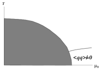
Figure 5: The phase diagram in the asymptotic, small-coupling region (unshaded). I have not differentiated between the different types of superconducting phases, marked here as $\langle qq\rangle\not=0$.

The basic principle behind the BCS theory of superconductivity is that, at finite density and zero temperature, attractive interactions between charged fermions lead to superconductivity, even if those attractive interactions are arbitrarily weak. The attraction causes the charged fermions to bind into charged Cooper pairs, and those Cooper pairs condense into a Bose condensate. In particle physics language, the Cooper pairs play the role of Higgs particles, the Cooper pair field $\psi\psi$ then acquires a VEV, and that VEV gives mass to the photon. A mass means a Yukawa potential, which is why magnetic fields fall of exponentially quickly inside a superconductor. This is the Meisner effect. In our case, the relevant fermions are quarks, the charge of interest is the color charge, and the corresponding “photons” are gluons.

In weak coupling, one can write a self-consistency equation for the formation of a condensate $\langle qq\rangle$ of the Cooper pairs. That equation is known as the gap equation and is depicted schematically in fig. 6, where $\Delta$ represents the condensate (or “gap”). If you iterate the gap equation, you can generate rainbows of gauge interaction lines. These diagrams represent repeated interactions of the two fermions, binding them into the Cooper pair, as depicted in fig. 7a.

Figure 6: The gap equation for the $\langle qq\rangle$ condensate.

Figure 7: (a) binding of a Cooper pair by multiple interactions; (b) a single such interaction.

Let’s now look at an individual interaction between the fermions, as in fig. 7b. This is just Coulomb scattering, and Coulomb scattering is naively infrared divergent. This divergence is a manifestation of the long-range nature of the Coulomb force. Consider first the case of electric interactions. Completely analogous to our earlier discussion about high temperature, electric fields are screened at finite density by the Debye effect (with the inverse Debye length $m_{\rm D}$ of order $g\mu$). The Debye effect cuts off the Coulomb divergence for electric interactions.

Now consider magnetic interactions between the two fermions. Again analogous to high temperature systems, static magnetic fields are not screened. In the old days of studying color conductivity, people simply assumed by analogy with the high-temperature case that there must be a scale $g^{2}\mu$ (analogous to $g^{2}T$) of non-perturbative magnetic physics, and that this non-perturbative physics would somehow cut off the magnetic Coulomb divergence. I’m told it was understood by a fellow named Barrois as early as 1979 that this is incorrect, but he could never get this result from his Ph.D. thesis published. Barrois left the field. The correct understanding of what cuts off the magnetic Coulomb divergence is recent. In 1998, Son^? realized that it is the screening of dynamical magnetic fields, due to Lenz’s Law, which I discussed earlier. Knowing the correct physics, he was able to then compute the size of the super-conducting gap at zero temperature, to leading order in the (assumed small) coupling $g(\mu)$:

$$\Delta=\#g^{-5}\mu\exp\left[-{3\pi^{2}\over\sqrt{2}\,g(\mu)}\right].$$ (11)

This formula puts a quantitative face on the assertion that QCD forms a color superconductor at sufficiently high density. One would still like to solve rigorously for what type (2SC, CFL, etc.) of superconductor it is, and that turns out to depend on the numerical coefficient $\#$ in front of (11). And that turns out to be the outstanding problem for dense QCD at small coupling: to calculate the numerical prefactor and so definitively distinguish the fine structure of the phase diagram of fig. 5.

Acknowledgements

I would like to thank Krishna Rajagopal, Dam Son, and Thomas Schaefer for discussions concerning dense QCD that helped me prepare this talk. This presentation was supported by the U.S. Department of Energy under Grant No. DE-FG02-97ER41027.

References

I have made no attempt to take on the mammoth task of citing even the most important works in the field, but I provide references for some particular statements made in the text.

References

- [1] For reviews, see, for example, A. Cohen, D. Kaplan and A. Nelson, Annu. Rev. Nucl. Part. Sci. 43, 27 (1993); V. Rubakov and M. Shaposhnikov, Usp. Fiz. Nauk 166, 493 (1996) [Phys. Usp. 39, 461 (1996)]; M. Trodden, Rev. Mod. Phys. 71, 1463 (1999).
- [2] See, for example, E. Braaten and A. Nieto, Phys. Rev. D 51, 6990 (1995); 53, 3421 (1996); and references therein.
- [3] D. Bödeker, Phys. Lett. B426, 351 (1998).
- [4] See, for example, G. Baym, H. Monien, C.J. Pethick and D.G. Reavenhall, Phys. Rev. Lett. 64, 1867 (1990).
- [5] G. Moore, C. Hu and B. Müller, Phys. Rev. D58, 045001 (1998); G. Moore and K. Rummukainen, Phys. Rev. D61, 105008 (2000); D. Bd̈eker, G. Moore and K. Rummukainen, Phys. Rev. D61, 056003 (2000).
- [6] E. Dagatto, F. Karsch and A. Moreo, Phys. Lett. B 169, 421 (1986); J. Kogut, M. Stephanov, and D. Toublan, hep-ph/9906346; and references therein.
- [7] M. Alford, A. Kapustin and F. Wilczek, Phys. Rev. D59, 054502 (1999); D. Son and M. Stephanov, hep-ph/0005225 (unpublished); and references therein.
- [8] K. Rajagopal, Nucl. Phys. A661, 150 (1999).
- [9] B. Barrois, Ph.D. thesis, report UMI 79-0847 (1979) (unpublished).
- [10] D. Son, Phy. Rev. D59, 094019 (1999).
- [11] T. Schäfer, Nucl. Phys. B575, 269 (2000).
- [12] W. Brown, J. Liu and H. Ren, Phys. Rev. D62, 054016 (2000).