IPPP/00/01

DTP/00/58

16 October 2000

Luminosity monitors at the LHC

V.A. Khoze^a, A.D. Martin^a, R. Orava^b and M.G. Ryskin^a,c

^a Department of Physics and Institute for Particle Physics Phenomenology, University of Durham, Durham, DH1 3LE

^b Department of Physics, University of Helsinki, and Helsinki Institute of Physics, Finland

^c Petersburg Nuclear Physics Institute, Gatchina, St. Petersburg, 188300, Russia

We study the theoretical accuracy of various methods that have been proposed to measure the luminosity of the LHC $pp$ collider, as well as for Run II of the Tevatron $p\bar{p}$ collider. In particular we consider methods based on (i) the total and forward elastic data, (ii) lepton-pair production and (iii) $W$ and $Z$ production.

1 Introduction

The Large Hadron Collider (LHC) being constructed at CERN, will generate proton-proton collisions with total c.m. energy of 14 TeV with a design luminosity $\mathcal{L}$ $=10^{34}$ cm^-2 s^-1. The experiments at this new facility will have a high potential to discover New Physics and to make various precision measurements, see, for example [1, 2]. Both the general purpose $pp$ experiments, ATLAS [3] and CMS [4], will provide high statistics data samples, and the accuracy of the precision measurements will be limited by systematic effects and, in many cases, by the uncertainty in the measurement of the luminosity $\mathcal{L}$. For example, precision measurements in the Higgs sector of typical accuracy of about 7%, for a wide range of possible Higgs mass, require the uncertainty in the luminosity to be $\leq 5\%$ [2]. Both LHC experiments are aiming at measuring the luminosity to 5%. Recall also that the enhancement in luminosity that will be achieved in Run II of the Fermilab Tevatron $p\bar{p}$ - collider will herald a new era of precision studies [5, 6, 7].

An obvious requirement for the success of these precision measurements is that the uncertainties in the theoretical calculations of the cross sections for the basic processes, which are to be used to determine the luminosity, should match the desired experimental accuracies.

In general, there are two possibilities to determine the luminosity – either (i) to measure a pair of cross sections which are connected quadratically with each other, or (ii) to measure a cross section whose value is well known or which may be calculated with good accuracy. The well-known example of the first possibility is the measurement of the total $\sigma_{\rm{tot}}$ and differential forward elastic cross sections which are related by the optical theorem; see, for example, [5, 8] for recent experimental discussions. This method is discussed further in Section 2.

Two types of processes stand out as examples of the second possibility to measure the luminosity. First there is exclusive lepton-pair production via photon-photon fusion

$$\stackrel{{\scriptstyle}}{{p}}\stackrel{{\scriptstyle(-)}}{{p}}\rightarrow\ \stackrel{{\scriptstyle}}{{p}}+\ l^{+}l^{-}\ +\stackrel{{\scriptstyle(-)}}{{p}}$$ (1)

where $l=e$ or $\mu$. To the best of our knowledge this proposal originated in [9]. A luminometer for the LHC based on measuring forward $e^{+}e^{-}$ pairs (of invariant mass $M_{ee}<10-20$ MeV and transverse momentum $p_{t}(ee)<10-20$ MeV) was proposed in [10], while Ref. [11] concerns the central production of $\mu^{+}\mu^{-}$ pairs (with $\left<M_{\mu\mu}\right>\ \sim$ 20 GeV and $p_{t}(\mu\mu)\sim$ 10–50 MeV). Lepton-pair production is the subject of Section 3.

Nowadays attention has also focussed on $W$ and $Z$ production as a possible luminosity monitor, both for Run II at the Tevatron and for the LHC see, for example, [12]. The reason is that the signal is clean, and the production cross sections are large and can now be calculated with considerable theoretical accuracy. We discuss this possibility further in Section 4.

In principle, we may monitor the luminosity using any process, with a significant cross section, which is straightforward to detect. For example, it could be single- (or two-) pion inclusive production in some rapidity and $p_{t}$ domain (for example $p_{t}=5-10~{}{\rm GeV};|\eta|<1$) or inclusive $\mu^{+}\mu^{-}$ production in a well-defined kinematic domain, etc. In this way we may control the relative luminosity and then calibrate the “monitor” by comparing the number of events detected for the “monitor” reaction with the number of events observed for a process with a cross section which is already known, or which may be calculated with sufficient accuracy.

For some applications better accuracy can be achieved by measuring the parton-parton luminosity. A discussion is given in Section 5. Finally, Section 6 contains our conclusions.

2 Elastic scattering

First we discuss the classic method to measure the luminosity, that is using the observed total and forward elastic $pp$ (or $p\bar{p}$) event rates. Neglecting Coulomb effects, the elastic cross section is given by

$$\left.\frac{d\sigma_{\rm el}}{dt}\right|_{t=0}\;=\;\frac{\sigma_{\rm tot}^{2}}{16\pi}\>(1+\rho^{2}).$$ (2)

The ratio $\rho$ of the real to the imaginary parts of the forward amplitude is small at Tevatron-LHC energies and can be estimated via dispersion relation techniques

$$\rho\;\simeq\;\frac{\pi}{2}\>\frac{\partial\ln\sigma_{\rm tot}(s)}{\partial\ln s}.$$ (3)

For example, at the LHC energy, $\sqrt{s}=14~{}{\rm TeV}$, it is predicted to be $\rho=0.10-0.12$; for a recent estimate, see, for example, Ref. [15]. Even the largest conceivable uncertainty in $\rho,$ that is $\Delta\rho=\pm 0.02$, leads only to an uncertainty of less than 0.5% in $d\sigma_{\rm el}/dt$. Thus if we measure the number of events corresponding to the elastic scattering and to the total cross section, then we may determine both the luminosity ${\cal L}$ and $\sigma_{\rm tot}$ (since $N_{\rm el}\propto\sigma_{t}^{2}{\cal L}$, whereas $N_{\rm tot}\propto\sigma_{t}{\cal L}$). The main problem in that it is extremely difficult to make measurements at the LHC in the very forward region, and so it is necessary to extrapolate elastic data from, say, $|t|\lower 3.01385pt\hbox{$\;\stackrel{{\scriptstyle\textstyle>}}{{\sim}}\;$}0.01~{}{\rm GeV}^{2}$ to $t=0$.

On the other hand it was found at the ISR that the observed ‘local’ slope

$$B(t)\;\equiv\;\frac{d\ln(d\sigma_{\rm el}/dt)}{dt}$$ (4)

depends on $t$. In particular at $\sqrt{s}=62~{}{\rm GeV}$ [16]

$$\Delta B\;=\;B(0)-B(|t|=0.2~{}{\rm GeV}^{2})\;\simeq\;2~{}{\rm GeV}^{-2}.$$ (5)

Note that if this $t$ dependence were to be solely due to a non-linear Pomeron trajectory [17], then the difference (5) would increase as the logarithm of the energy $(\ln s)$; giving, for example, $\Delta B\simeq 4.8~{}{\rm GeV}^{-2}$ at the LHC energy. The $t$-dependence of the local slope $B(t)$ has recently been determined [15] using a model which incorporates all the main features of high energy soft diffraction. That is the model embodies

• the pion-loop contribution to the Pomeron pole (which is the main source of the non-linearity of the Pomeron trajectory $\alpha_{I\!\!P}(t)$),

• a two-channel eikonal to include the Pomeron cuts which are generated by elastic and quasi-elastic (with $N^{*}$ intermediate states) $s$-channel unitarity,

• the effects of high-mass diffractive dissociation.

The parameters of the model are $\alpha(0)$ and $\alpha^{\prime}$ of the bare Pomeron trajectory, two parameters describing the elastic proton-Pomeron vertex, and the triple-Pomeron coupling and its slope [15]. The values of the parameters were tuned to describe the observed $pp$ (or $p\bar{p}$) elastic differential cross sections throughout the ISR-Tevatron range, restricting the description to the forward region $|t|<0.5~{}{\rm GeV}^{2}$. Note that there are two effects, leading to a $t$ dependence of $B$, which act in opposite directions. First, the non-linear pion-loop contributions [17] to the Pomeron trajectory, $\Delta\alpha_{I\!\!P}(t)$, lead to a contribution $\Delta B_{I\!\!P}(t)=\Delta\alpha_{I\!\!P}(t)\ln s$ in single Pomeron exchange, which increases as $|t|\rightarrow 0$. On the other hand the absorptive (rescattering) corrections, associated with eikonalization, lead to a dip in $d\sigma_{\rm el}/dt$ (whose position moves to smaller $|t|$ as the collider energy, $\sqrt{s}$, increases), with the result that the local slope $B(t)$ grows as $-t$ approaches the position of the diffractive minimum; that is $B(t)$ decreases as $|t|\rightarrow 0$. Fortunately, just at the LHC energy, these two effects almost compensate each other.

So far it has proved impossible to sum up in a consistent way all the multi-Pomeron diagrams. For this reason two versions of the model were studied in Ref. [15] with maximal and minimal contributions from high-mass diffractive dissociation. After tuning the values of the parameters to describe the $\sigma_{\rm tot}$ and the forward $d\sigma_{\rm el}/dt$ data, the two versions of the model predict different values of the slope at $t=0,B(0)$. The maximal choice gives a larger value $B(0)=21.9~{}{\rm GeV}^{-2}$, while for the minimal case we obtain $B(0)=20.3~{}{\rm GeV}^{-2}$. However in both cases the variation of $B(t)$ satisfies $\Delta B<0.2~{}{\rm GeV}^{-2}$ for $|t|<0.1~{}{\rm GeV}^{2}$, or $\Delta B<0.1~{}{\rm GeV}^{-2}$ for the more restricted interval $0<|t|<0.02~{}{\rm GeV}^{2}$. It means that we may neglect such a small variation of $B(t)$ with $t$ and safely extrapolate the observed cross section $d\sigma_{\rm el}/dt$ down to $t=0$, using the slope measured, say, in the interval $0.01<|t|<0.05~{}{\rm GeV}^{2}$. The error, due to the variation of $B$ with $t$, is expected to be less than $\Delta B\cdot|t|\lower 3.01385pt\hbox{$\;\stackrel{{\scriptstyle\textstyle<}}{{\sim}}\;$}0.2\%$.

In the very forward region, $|t|\sim 0.01-0.02~{}{\rm GeV}^{2}$, it may only be possible to measure the elastic cross section in an LHC run with a rather low luminosity. For the high luminosity runs one would then have to use another monitor. One possibility is to choose a single particle inclusive process, with a significant cross section, and “calibrate” it in the low luminosity run by comparing with the total and elastic cross sections discussed above. It would be even better if we were able to calibrate several different reactions. Then to use, as a luminosity monitor, the reaction with the closest topology (or kinematic configuration) to the process that we are to study in the high luminosity run.

3 Lepton pair production as a luminometer

At first sight any QED process, with sufficient event rate, may be used as a luminosity monitor. Up to ISR energies the luminosity was measured via Coulomb elastic $pp$ scattering, where at very small $|t|$ the influence of the dominant single photon exchange contribution is evident. Unfortunately, in the LHC environment, the Coulomb interference region, $|t|\lower 3.01385pt\hbox{$\;\stackrel{{\scriptstyle\textstyle<}}{{\sim}}\;$}(1-3)\times 10^{-4}~{}{\rm GeV}^{2}$ is not likely to be experimentally accessible.

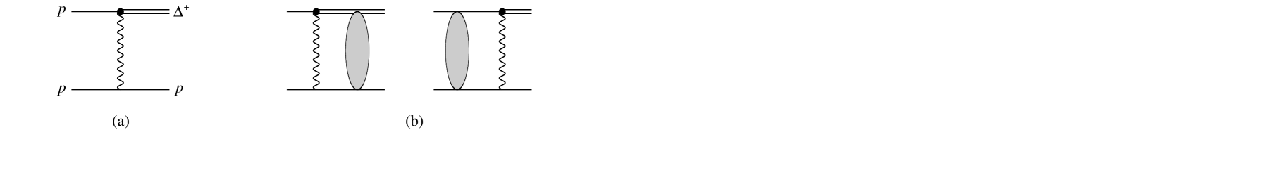
Figure 1: (a) $\Delta^{+}$ production mediated by photon exchange, and (b) possible rescattering corrections.

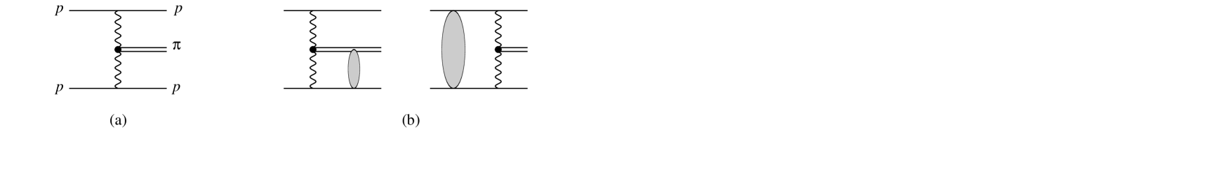
Figure 2: (a) $\pi^{0}$ production mediated by photon exchanges and (b) two of the possible rescattering corrections.

Other possibilities to consider are $\Delta$ isobar Coulomb excitation, ($pp\rightarrow\Delta^{+}p$), or $\pi^{0}$ and $\eta$ production, which are all mediated by photon exchange, as shown in Figs. 1(a) and 2(a) respectively. Surprisingly, the electromagnetic widths $\Delta^{+}\rightarrow p\gamma,\pi^{0}\rightarrow\gamma\gamma$ and $\eta\rightarrow\gamma\gamma$ are known only to 7–10% accuracy [18]. Moreover, strong interaction effects in the initial and final states give non-negligible corrections, see Figs. 1(b) and 2(b).

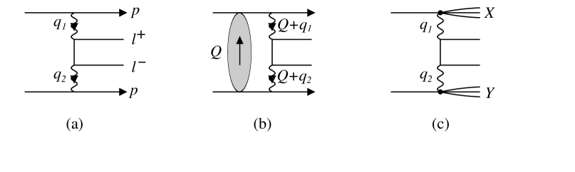
Figure 3: (a) Lepton pair production in $pp$ collisions, (b) one of the rescattering corrections, and (c) a possible contamination coming from proton dissociation into $X,Y$ systems.

Lepton pair production looks much more promising as a luminosity monitor. The Born amplitude of Fig. 3(a) may be calculated within pure QED (see, for example, the reviews in [19]), and there are no strong interactions involving the leptons in the final state. The only question is the size of the absorptive corrections arising from inelastic proton-proton rescattering, sketched in Fig. 3(b). Fortunately the rescattering correction is suppressed for two reasons. First, the main part of the Born cross section (Fig. 3(a)) comes from the peripheral region with large impact parameter $b_{t}$, where the strong amplitude $A(s,b_{t})$ is small. Second, even in the small $b_{t}$ domain, the rescattering correction is greatly suppressed due to the angular integration.

Before we discuss the last point, we note that, in practice, it is difficult to exclude contributions coming from the reactions

$$pp\rightarrow X+l^{+}l^{-}+p$$

$$pp\rightarrow X+l^{+}l^{-}+Y$$ (6)

where $X$ and $Y$ are baryon excitations, that is $N^{*}$ or $\Delta$ isobars. Of course the matrix elements of the corresponding processes (such as Fig. 3(c)) can, in principle, be determined from photoproduction and deep inelastic data, and may be taken into account. However the matrix elements of Fig. 3(c) are not known to sufficient accuracy and it is better to suppress the contributions of (3) by experimental cuts. The procedure is as follows. Recall that, due to gauge invariance, inelastic vertices of the type $p\rightarrow X+\gamma$ vanish like [19]

$$V(p\rightarrow X\gamma)\ \propto\ q_{1t}$$ (7)

as the photon transverse momentum $q_{1t}\rightarrow 0$. Unfortunately it is difficult to measure a leading proton with very small transverse momentum, that is $q_{t}\lower 3.01385pt\hbox{$\;\stackrel{{\scriptstyle\textstyle<}}{{\sim}}\;$}10-30~{}{\rm MeV}$. So to take advantage of the behaviour of (7), it was proposed [11] to select events with very small transverse momentum of the lepton pair

$$p_{t}\equiv\left|\ \mbox{\boldmath$q$}_{l^{+}t}+\mbox{\boldmath$q$}_{l^{-}t}\ \right|<10-30\rm{MeV},$$ (8)

in order to suppress $N^{*}$ and $\Delta$ production. In such a case the integral over the transverse momenta of the photons in the Born cross section of Fig. 3(a) takes the form

$$\int\>\frac{dq_{1t}^{2}\>dq_{2t}^{2}\>q_{1t}^{2}\>q_{2t}^{2}}{(q_{1t}^{2}\>+\>t_{1})^{2}(q_{2t}^{2}\>+\>t_{2})^{2}}\>\delta^{(2)}(\mbox{\boldmath$p$}_{t}-\mbox{\boldmath$q$}_{1t}-\mbox{\boldmath$q$}_{2t})\>d^{2}p_{t},$$ (9)

where the dominant contributions come from the regions $q_{it}\lower 3.01385pt\hbox{$\;\stackrel{{\scriptstyle\textstyle<}}{{\sim}}\;$}p_{t}$. The values of the longitudinal components are

$$t_{i}\equiv\left|t_{i,min}\right|=x^{2}_{i}m^{2}_{p},$$ (10)

where $x_{i}$ are the fractions of the momenta of the incoming protons carried by the $l^{+}l^{-}$ pair, and $m_{p}$ is the mass of the proton.

3.1 $\mu^{+}\mu^{-}$ production

To identify muons (and to separate them from $\pi^{\pm}$ mesons) it is necessary to observe charged particles after they have transversed a thick (iron) absorber. It means that we consider only muons which have a rather large transverse energy $E_{t}\lower 3.01385pt\hbox{$\;\stackrel{{\scriptstyle\textstyle>}}{{\sim}}\;$}5$ GeV. However, it is still possible to select events where the sum of their transverse momenta is small, $p_{t}<30$ MeV. In this case

$$x_{i}\simeq(2-3)E_{t}/\sqrt{s}\simeq 10^{-3},\ \ \ \ \ t_{i}\simeq 10^{-6}\rm{GeV}^{2},$$ (11)

at the LHC energy. In such a configuration the main contribution to the integral (9) comes from the domains $q_{1t}\approx p_{t},~{}t_{2}\ll q_{2t}^{2}\ll p_{t}^{2}$ and $q_{2t}\approx p_{t},~{}t_{1}\ll q_{1t}^{2}\ll p_{t}^{2}$. Performing the $q_{it}^{2}$ integrations in these two domains gives $\ln(p_{t}^{2}/t_{2})$ and $\ln(p_{t}^{2}/t_{1})$ respectively, and so the Born cross section behaves as

$$\frac{d\hat{\sigma}}{dp^{2}_{t}}\ \propto\ \frac{1}{p^{2}_{t}}\ {\rm ln}\left(\frac{p^{4}_{t}}{t_{1}t_{2}}\right)$$ (12)

In addition to the use of the small $p_{t}$ cut in order to separate the elastic process (1) from the excitation process (3), we can also exploit the different kinematics of the processes. For example in [11] it was proposed to fit the observed distribution in the muon acoplanarity angle $\phi$ in order to isolate the elastic mechanism via its prominent peak at $\phi=0$.

3.2 Absorptive corrections to $l^{+}l^{-}$ production

To determine the effect of the absorptive, or re-scattering, correction, we calculate diagram 3(b) with an extra loop integration over the momentum $Q$ transferred via the strong interaction amplitude shown by the “blob”. The relative size of the correction, to the amplitude for lepton-pair production of Fig. 3(a), is

$$\delta\;=\;\frac{(\sigma_{\rm inel}/8\pi^{2})\int d^{2}Q_{t}d^{2}q_{1t}d^{2}p_{t}\hat{\sigma}(q_{1},q_{2};q_{1}+Q,q_{2}+Q)\>F(Q)}{\int d^{2}q_{1t}d^{2}p_{t}\hat{\sigma}(q_{1},q_{2};q_{1},q_{2})\>F(0)},$$ (13)

where $F(Q)$ represents the collective effect of the appropriate proton electromagnetic form factors $F_{N}$ and the $Q^{2}$ dependence of the strong interaction amplitude

$$F(Q)\;=\;F_{N}(q_{1}^{2})\>F_{N}(q_{2}^{2})\>F_{N}((Q+q_{1})^{2})\>F_{N}((Q+q_{2})^{2})\>e^{bQ^{2}/2}.$$ (14)

$b$ is the slope of the $pp$ elastic cross section, that is $d\sigma_{\rm el}/dt\propto\exp(bt)$. We can interpret the correction $\delta$ in terms of $S=1-\delta$, where $S$ is the “survival probability amplitude” that the secondary hadrons produced in the soft rescattering do not accompany $\ell^{+}\ell^{-}$ production. Of course this effect is due to the inelastic strong interaction only. Consider the hypothetical case with pure elastic $pp$ rescattering (at fixed impact parameter $b_{t}$, that is for fixed partial wave $\ell=b_{t}\sqrt{s}/2$). Then elastic rescattering only changes the phase of the QED matrix element, ${\cal M}\rightarrow{\cal M}\exp(2i\phi_{\ell})$, and does not alter the QED cross section $\sigma=|{\cal M}|^{2}$. Thus we have to account only for the inelasticity of the strong interaction, that is $\delta\propto\sigma_{\rm inel}$ as in (13). Throughout this paper we do not discuss the effects of “pile-up” events. Thus there will be an additional factor $(W<1)$ which represents the probability not to include events with extra secondaries coming from an almost simultaneous interaction of another pair of protons. Experimentally the depletion due to such pile-up events may be overcome, for example, by cleanly observing the vertex of $\mu^{+}\mu^{-}$ production.

The cross section $\hat{\sigma}$ in (13) plays the role of the cross section for the QED subprocess of $\gamma\gamma$ scattering through the lepton box. For the absorptive process, the photons have momenta $q_{1}+Q$ and $q_{2}+Q$ in the “left” amplitude $A$ shown in Fig. 3(b), and $q_{1},q_{2}$ in the “right” amplitude $A^{*}$, which is not shown. Here we have assigned the absorptive effect to $A$. Actually the numerator of (13), and the symbolic diagram 3(b), summarize a set of Feynman graphs which describe the effects of the strong interaction between the protons in the amplitude $A$. Then we have to add the equivalent set of diagrams in which the rescattering effects occur in the amplitude $A^{*}$. The total correction to (12) is therefore $2\delta d\hat{\sigma}/dp_{t}^{2}$. The rescattering correction is due to the imaginary part of the strong amplitude only. The effects coming from the real part in $A$ cancel with those in $A^{*}$.

At first sight the largest absorptive effects, (13), appear to come from the largest values of $Q_{t}\lower 3.01385pt\hbox{$\;\stackrel{{\scriptstyle\textstyle<}}{{\sim}}\;$}1/R_{p}$, where $R_{p}$ is the proton radius; higher values of $Q_{t}$ are cut-off by the proton form factor. However when $Q_{t}\gg q_{1t},q_{2t}$ an interesting suppression occurs. In this domain $\gamma\gamma\rightarrow l^{+}l^{-}$ occurs dominantly in the $J_{z}=0$ two-photon state. The projection of the orbital angular momentum on the longitudinal $(z)$ axis is clearly zero, while the spin (which originates from the photon polarisations) is described by the tensor $Q_{\mu t}Q_{\nu t}$. After the azimuthal integration, the tensor takes the form $\frac{1}{2}Q^{2}\delta^{\bot}_{\mu\nu}$, leading to $J_{z}=0$. If we neglect the mass of the lepton, $m_{l}\ll E_{t}$, and higher order QED corrections, then the Born amplitude, with $J_{z}=0$, vanishes. This is a well known result, see, for example, [23]. As shown in Ref. [24], the physical origin of the suppression is related to the symmetry properties of the $J_{z}=0$ Born amplitude.

The “cross section” $\hat{\sigma}(q_{1},q_{2};q_{1}+Q,q_{2}+Q)$ for our QED subprocess depends on the transverse momenta of four virtual photons. The full expression for $\hat{\sigma}$ is rather complicated. However in the limit $E_{t}\gg q_{1t},q_{2t},Q_{t},m_{l},$ we can integrate over the direction of the lepton transverse momentum $\mbox{\boldmath$k$}_{t}$ (with $|\mbox{\boldmath$k$}_{t}|\simeq E_{t}$), and the formula reduces to the simple form

$$\hat{\sigma}\propto\frac{{\rm cosh}(\Delta\eta)}{E^{4}_{t}{\rm cosh}^{4}(\frac{1}{2}\Delta\eta)}\ \ \frac{\left[(Q+q_{2},q_{1})(Q+q_{1},q_{2})+(Q+q_{1},q_{1})(Q+q_{2},q_{2})-(q_{1},q_{2})(Q+q_{1},Q+q_{2})\right]}{q^{2}_{1}q^{2}_{2}(Q+q_{1})^{2}(Q+q_{2})^{2}}$$ (15)

where the notation $(k_{1},k_{2})$ is used for the scalar product of two transverse vectors, and where the rapidity difference

$$\Delta\eta\equiv\left|\eta(l^{+})-\eta(l^{-})\right|.$$ (16)

It is interesting to note that the dependence of the cross section $\hat{\sigma}$ on $q_{1t},~{}q_{2t}$ and $Q_{t}$ follows directly from the symmetry properties of the process. First, gauge invariance implies that $\hat{\sigma}$ must vanish when the transverse momentum of any photon goes to zero. That is $\hat{\sigma}$ must contain a factor $q_{1t}q_{2t}(Q+q_{1})_{t}(Q+q_{2})_{t}$. Next, it has to be symmetric under the interchanges $q_{1}\leftrightarrow q_{2}$ and $q_{i}\leftrightarrow(Q+q_{i})$. Finally, as discussed above, in the limit $Q_{t}\gg q_{1t},q_{2t}$, it must vanish after the azimuthal angular integration of $\mbox{\boldmath$Q$}_{t}$ has been performed. The only possibility to satisfy these conditions, to lowest order in $Q_{t}/E_{t}$ and $q_{it}/E_{t}$, is given by the expression in square brackets in (15). To obtain the $\Delta\eta$ and $E_{t}$ behaviour, shown in the first factor in $\hat{\sigma}$ of (15), it is sufficient to put $Q_{t}=0$ and to recall the well known pure QED cross section.

Recall that for $\mu^{+}\mu^{-}$ production we select events with small transverse momentum of the lepton pair, $p_{t}$. Now if $\mbox{\boldmath$p$}_{t}=\mbox{\boldmath$q$}_{1t}-\mbox{\boldmath$q$}_{2t}\simeq 0$, that is if $Q_{t}\gg p_{t}$, then the last factor in expression (15) of the absorptive cross section simplifies to

$$\hat{\sigma}\ \propto\ \frac{\left[2(Q+q_{1},q_{1})^{2}-q^{2}_{1}(Q+q_{1})^{2}\right]}{\left[q^{2}_{1}(Q+q_{1})^{2}\right]^{2}},$$ (17)

which, upon integration over the azimuthal angle of the vector $(\mbox{\boldmath$Q$}+\mbox{\boldmath$q$}_{1})_{t}$, gives zero. Therefore the main contribution to (13) comes from values of $Q_{t}\approx p_{t}$, and the absorptive correction

$$\delta\approx\frac{\sigma_{\rm inel}}{8\pi}\ p^{2}_{t}\ C.$$ (18)

The coefficient $C$ is numerically small for two reasons. First, the integration over the loop momentum $Q_{t}$ kills the logarithmic factor, ln$(p^{4}_{t}/t_{1}t_{2})$, which enhanced the original cross section (12) in the absence of absorptive corrections. To see this, note that the $\log$ came from the $q_{t}^{2}dq_{t}^{2}/q_{t}^{4}$ integrations, for both $q_{1t}$ and $q_{2t}$, of (9), see (12). However when $Q_{t}\neq 0$ the integrands are of the form $\mbox{\boldmath$q$}_{t}\cdot(\mbox{\boldmath$Q$}_{t}+\mbox{\boldmath$q$}_{t})/q_{t}^{2}|\mbox{\boldmath$Q$}_{t}+\mbox{\boldmath$q$}_{t}|^{2}$, and there is no logarithmic singularity for either $q_{t}\rightarrow 0$ or $|\mbox{\boldmath$Q$}_{t}+\mbox{\boldmath$q$}_{t}|\rightarrow 0$. Second, there is a suppression of $C$ from cancellations which occur after integration over the remaining azimuthal angles. For example, if the invariant mass of the $\mu^{+}\mu^{-}$ pair produced at zero rapidity is $M_{\mu\mu}=20~{}{\rm GeV}$, then the value of the coefficient $C=0.14,0.13,0.09$ and 0.08 for $p_{t}=5,10,30$ and 50 MeV respectively. This leads to a negligible correction to the cross section (12), for example

$$2\delta\lower 3.01385pt\hbox{$\;\stackrel{{\scriptstyle\textstyle<}}{{\sim}}\;$}\frac{80{\rm mb}}{4\pi}\ p^{2}_{t}\ C<0.02\%~{}(0.13\%)$$ (19)

for $p_{t}=10$ MeV (30 MeV).

Note that the rescattering contribution of Fig. 3(b) is less singular as $q_{1t},q_{2t}\rightarrow 0$ than the pure QED term of Fig. 3(a). Therefore the rescattering correction does not induce a sharp peak at $\phi=0$ in the muon acoplanarity distribution. Thus removing the excitation processes (3) by fitting the $\phi$ distribution, will automatically suppress the rescattering correction.

3.3 $e^{+}e^{-}$ production

Unlike $\mu^{+}\mu^{-}$ production, for $e^{+}e^{-}$ production we do not need to select events with electrons of large transverse momentum $p_{et}$. Providing the energy of the electrons $E\sim 5~{}{\rm GeV}$, we may use, say, an electromagnetic calorimeter to identify them. Therefore we may consider the small $p_{et}$ domain where the $e^{+}e^{-}$ production cross section is much larger. The dominant contribution to the cross section comes from the region of $p_{et}$ of the order of the electron mass ($p_{et}\lower 3.01385pt\hbox{$\;\stackrel{{\scriptstyle\textstyle<}}{{\sim}}\;$}1$ MeV). As $p_{et}$ is small, we cannot neglect $Q_{t}$ in the $t$ channel electron propogator. As a consequence the integral over $Q_{t}$ becomes super-convergent

$$\int\frac{d^{2}Q_{t}|\mbox{\boldmath$Q$}_{t}+\mbox{\boldmath$q$}_{1t}|\>|\mbox{\boldmath$Q$}_{t}+\mbox{\boldmath$q$}_{2t}|}{(Q+q_{1})^{2}\>(Q+q_{2})^{2}\>(|Q+q_{1}+p_{e}|^{2}+m^{2}_{e})}.$$ (20)

It is informative to note the origin of this form. Due to gauge invariance, the numerator vanishes when the photon transverse momenta $|\mbox{\boldmath$Q$}_{t}+\mbox{\boldmath$q$}_{it}|\rightarrow 0$. The first two factors in the denominator arise from the photon propagators. Finally we have the factor due to the electron propagator, with $Q\simeq(0;\mbox{\boldmath$Q$}_{t},0)$. Contrary to $\mu^{+}\mu^{-}$ production, where the lepton propagator was driven by the large $p_{t}\simeq E_{t}$ of the muon, here the momentum $Q_{t}$ is not negigible in comparison with $p_{et}$ and the dominant contribution comes from the region $Q^{2}_{t}\simeq m^{2}_{e}<10^{-6}$ GeV². Hence the expected absorptive correction due to strong interaction rescattering is

$$2\delta\approx\frac{\sigma_{\rm inel}}{4\pi}\ Q^{2}_{t}\sim\frac{80{\rm mb}}{4\pi}\ 10^{-6}{\rm GeV}^{2}\lower 3.01385pt\hbox{$\;\stackrel{{\scriptstyle\textstyle<}}{{\sim}}\;$}10^{-5}$$ (21)

3.4 Conclusion on $l^{+}l^{-}$ production as a luminosity monitor

We see that both $\mu^{+}\mu^{-}$ and $e^{+}e^{-}$ pair production may be used as monitor processes in high luminosity LHC collisions. However we must employ special selection cuts on the $l^{+}l^{-}$ data. To suppress $N^{*}$ contamination we impose small transverse momentum $p_{t}$ of the lepton pair, moreover for $e^{+}e^{-}$ production we require the individual electron $p_{et}$ to be small. We also require the leptons to be sufficiently energetic in order to identify them. Then the cross section for $l^{+}l^{-}$ production at the LHC $(pp\rightarrow p+l^{+}l^{-}+p)$ can be calculated within pure QED and, importantly, we may neglect the strong rescattering effects between the protons up to $10^{-4}$ accuracy. Of course by requiring the muons to have high $E_{t}$ we have a rather small cross section. However here we may trace back the muon tracks and determine the interaction vertex, and hence isolate the interaction in pile-up events. So, in principle, $\mu^{+}\mu^{-}$ pair production, with high $E_{t}$ muons, may be used as a luminometer in very high luminosity LHC runs.

4 $W$ and $Z$ production as a luminosity monitor

$W$ and $Z$ production in high energy $pp$ and $p\bar{p}$ collisions have clean signatures through their leptonic decay modes, $W\rightarrow l\nu$ and $Z\rightarrow l^{+}l^{-}$, and so may be considered as potential luminosity monitors [12]. A vital ingredient is the accuracy to which the cross sections for $W$ and $Z$ production can be theoretically calculated. The cross sections depend on parton distributions, especially the quark densities, in a kinematic region where they are believed to be reliably known. Recent determinations of the $W$ and $Z$ cross sections can be found in Refs. [25, 26]. Here the situation has improved, and next-to-next-to-leading order (NNLO) predictions have been made. The most up-to-date values are reproduced in Fig. 4 [26] and Figs. 5,6 [25, 26].

To estimate the accuracy with which the $W$ and $Z$ cross sections are known, we start with Fig. 4. Fig. 4 was obtained using parton distributions found in LO, NLO and NNLO global analyses of the same data set [26]. It is relevant to summarize the contents of these plots. The predictions labelled LO, NLO and NNLO can be schematically written as follows

$$\sigma_{\rm LO} = f_{\rm LO}\otimes f_{\rm LO}$$

$$\sigma_{\rm NLO} = f_{\rm NLO}\otimes f_{\rm NLO}\otimes[1+\alpha_{S,{\rm NLO}}K^{(1)}]$$

$$\sigma_{\rm NNLO} = f_{\rm NNLO}\otimes f_{\rm NNLO}\otimes[1+\alpha_{S,{\rm NNLO}}K^{(1)}+(\alpha_{S,{\rm NNLO}})^{2}K^{(2)}]$$ (22)

where the label on $\alpha_{S}$ indicates the order to which the $\beta$-function is evaluated. The parton distributions $f$ obtained from the new global LO, NLO and NNLO analyses [26] correspond to $\alpha_{S}(M^{2}_{Z})=$ 0.1253, 0.1175 and 0.1161 respectively. The NLO and NNLO coefficient functions $K^{1,2}$ are known [27]. However, although the relevant deep inelastic coefficient functions are also known, there is only partial information on the NNLO splitting functions. Recently van Neerven and Vogt [28] have constructed compact analytic expressions for the NNLO splitting functions which represent the fastest and the slowest possible evolution that is consistent with the existing partial information. These expressions have been used to perform global parton analyses at NNLO [26]. The uncertainty in the NNLO predictions of $\sigma_{W}$ and $\sigma_{Z}$ due to the residual ambiguity in the splitting functions is shown by the width of the NNLO bands in Fig. 4. This amounts to about $\pm 1\%$ uncertainty at the LHC energy, and less at the Tevatron. For completeness, we note that the dashed lines in Fig. 4 correspond to the quasi-NLO prediction

$$\sigma_{{\rm NLO}^{\prime}}=f_{\rm NLO}\otimes f_{\rm NLO}\otimes[1+\alpha_{S,{\rm NLO}}K^{(1)}+(\alpha_{S,{\rm NLO}})^{2}K^{(2)}],$$ (23)

which was the best that could be done before the work of Refs. [28, 26].

We see that the LO $\rightarrow$ NLO $\rightarrow$ NNLO convergence of the predictions for $\sigma_{W,Z}$ is good. The jump from $\sigma_{\rm LO}$ to $\sigma_{\rm NLO}$ is mainly due to the well-known, large, $O(\alpha_{S})$ $\pi^{2}$-enhanced Drell-Yan K-factor correction, arising from soft-gluon emission. The NLO and NNLO cross sections are much closer and, if this was the end of the story, $W$ and $Z$ production can clearly be predicted with sufficient accuracy.

However let us turn to Figs. 5 and 6, each of which combine results presented in Refs. [25] and [26]. The solid squares and triangles show the additional uncertainty in the predictions for $\sigma_{W}$ and $\sigma_{Z}$ which arise from changing the input information in the global parton analyses. The two major uncertainties appear to be due to the value of $\alpha_{S}$ and to using different parton densities labelled by q$\uparrow$ and q$\downarrow$. The plots show the change in $\sigma_{W}$ and $\sigma_{Z}$ which is caused by changing the value of $\alpha_{S}(M^{2}_{Z})$ by $\pm 0.005$ respectively. The change in $\sigma_{W}$ and $\sigma_{Z}$ at the LHC energy is enhanced as compared to that at the Tevatron, since DGLAP evolution is more rapid at the smaller $x$ values, $x\sim M_{W,Z}/\sqrt{s}$, probed at the higher energy. However, with our present knowledge of $\alpha_{S}$, the uncertainty $\Delta\alpha_{S}=\pm 0.005$ is too conservative, and $\pm 2\%$ is a more realistic uncertainty in $\sigma_{W,Z}$ from this source at the LHC energy.

The normalisation of the input data used in the global parton analyses is another source of uncertainty in $\sigma_{W,Z}$. The HERA experiments provide almost all of the data used in the global analyses in the relevant small $x$ domain. The quoted normalisation uncertainties of the measurements of the proton structure function $F_{2}$ from the H1 and ZEUS experiments vary with $Q^{2}$, but a mean value of $\pm 2.5\%$ is appropriate. The q$\uparrow$ and q$\downarrow$ parton sets correspond to separate global fits in which the HERA data have been renormalised by $\pm 2.5\%$ respectively. For $W$ and $Z$ production, of $q\bar{q}$ origin, we naively would expect this to translate into a $\pm 5\%$ variation in $\sigma_{W,Z}$, but the effect of DGLAP evolution up to $Q^{2}\sim M^{2}_{W,Z}$ is to suppress the difference in the predictions.

In summary, allowing for all the above uncertainties, we conclude that the cross sections of $W$ and $Z$ production are known to $\pm 4\%$ at the LHC energy, and to $\pm 3\%$ at the Tevatron. A major contributer to this error is the uncertainty in the overall normalisation of the H1 and ZEUS measurements of $F_{2}$. The normalisation may be made more precise by experiments in Run II at the Tevatron.

5 Parton-parton luminosity

In some circumstances it is sufficient to know the parton-parton luminosity, and not the proton-proton luminosity, see, for example, [12]. Of course if the proton-proton luminosity is known then the parton-parton luminosities can be calculated from the parton distributions determined in the global parton analyses. However in this case we rely on the normalisation of experiments at previous accelerators which yielded data that were used in the global analyses.

Thus it may be better to monitor the parton-parton luminosities directly in terms of a subprocess which can be predicted theoretically to high precision. The best example is inclusive $W$ (or $Z$) boson production, which is predicted up to two-loops, that is to NNLO [26]. The accurate observation of $W$ (or $Z$) production at the LHC may therefore be used to determine the quark-antiquark luminosity. Then the gluon flux, for example, may be determined from the global parton analysis which already is made to describe the measured $W$ (or $Z$) cross sections. One advantage of this technique is that, for most LHC applications such as the search for new heavy particles, we need to consider a smaller interval of DGLAP evolution than has been the practice hitherto.

Other ways to constrain the gluon-gluon luminosity are to study $t\bar{t}$ production or the production of two large $p_{t}$ prompt photons. The leading order subprocess is $q\bar{q}\rightarrow\gamma\gamma$. However at LHC energies the $gg\rightarrow\gamma\gamma$ box diagram gives an important contribution. The two diagrams are shown in Fig. 7. The relative contributions are shown in Fig. 8 as a function of the transverse momentum of the photon pair $\mbox{\boldmath$p$}_{t}=\mbox{\boldmath$q$}_{\gamma 1t}+\mbox{\boldmath$q$}_{\gamma 2t}$ for the case when each photon has transverse momentum $q_{\gamma t}>20~{}{\rm GeV}$ and rapidity $|\eta_{\gamma}|<1$. We see that in this kinematic domain the $gg\rightarrow\gamma\gamma$ subprocess gives a major contribution due to the higher $gg$ luminosity. However there is a strong possibility of contamination by the subprocess $gq\rightarrow\gamma\gamma q$, unless severe photon isolation cuts are imposed, see, for example, Ref. [1].

So far we have considered conventional parton distributions $a(x,\mu^{2})$ integrated over the parton transverse momentum $k_{t}$ up to the factorization scale $\mu$. However many reactions are described by unintegrated distributions $f_{a}(x,k_{t}^{2},\mu^{2})$ which depend on both $k_{t}$ and the longitudinal momentum fraction $x$ carried by the parton. In principle, unintegrated distributions are necessary for the description of all processes which are not totally inclusive. In these cases, instead of the conventional QCD factorization, we have $k_{t}$ factorization [31]. Indeed, for some processes, after the specific integration over $k_{t}$, the conventional ‘hard’ QCD factorization may be destroyed.

The unintegrated quark-quark luminosity may be determined, for example, by observing the $k_{t}$ distribution of $W$ (or $Z$) bosons or Drell-Yan pairs. At leading order, the $k_{t}$-dependence of cross sections is given by the convolution

$$\frac{d\sigma}{d^{2}k_{t}}\;\propto\;\int\>\frac{d^{2}p_{1}}{p_{1}^{2}}\>\frac{d^{2}p_{2}}{p_{2}^{2}}\>\delta^{(2)}(\mbox{\boldmath$p$}_{1}+\mbox{\boldmath$p$}_{2}-\mbox{\boldmath$k$}_{t})\>f_{q}(x_{1},p_{1}^{2},\mu^{2})\>f_{\bar{q}}(x_{2},p_{2}^{2},\mu^{2}).$$ (24)

At large $k_{t}\gg\Lambda_{\rm QCD}$, to leading $\ln k_{t}$ order, the dominant contribution comes from either the domain $p_{1}\approx k_{t},~{}p_{2}\ll k_{t}$ or the domain $p_{2}\approx k_{t},~{}p_{1}\ll k_{t}$. It is natural to choose the factorization scale $\mu\approx k_{t}$. Then the $k_{t}$ distribution takes the simple form [32]

$$\frac{d\sigma}{d^{2}k_{t}}\;\propto\;\left[x_{1}q_{1}(x_{1},k_{t}^{2})\>f_{\bar{q}}(x_{2},k_{t}^{2},k_{t}^{2})\>+\>x_{2}\bar{q}_{2}(x_{2},k_{t}^{2})\>f_{q}(x_{1},k_{t}^{2},k_{t}^{2})\right],$$ (25)

since at leading order

$$\int^{k_{t}^{2}}\>\frac{dp^{2}}{p^{2}}\>f_{a}(x,p^{2},k_{t}^{2})\;=\;xa(x,k_{t}^{2}).$$ (26)

Moreover diffractive processes (with one or more rapidity gaps) are described, in general, by skewed parton distributions. An example is the double-diffractive exclusive Higgs boson production, described by the Feynman diagram shown in Fig. 9. This process is described by skewed gluon distributions with $x_{1}\neq x_{1}^{\prime}$ and $x_{2}\neq x_{2}^{\prime}$ [33, 34].

Sometimes even the “skewed” parton flux can be monitored directly via another process with similar kinematics. For example, we may monitor the effective Pomeron-Pomeron luminosity for Higgs production of Fig. 9 by measuring double- diffractive dijet production in the region in which the transverse energy of the jets ($E_{t}$) is of about half that of the Higgs mass $(E_{t}\sim M_{H}/2)$ [34, 35].

Fortunately most of the physically relevant processes are described by skewed distributions with $x_{i}\ll 1$. In these cases the skewed distributions may be reliably reconstructed from the known conventional parton distributions [36].

6 Conclusions

We have studied the theoretical accuracy of the main three proposals for determining the luminosity of the LHC $pp$ collider — namely using forward elastic data, lepton-pair production and $W$ or $Z$ boson production. The desired goal of a measurement to within $\pm 5\%$ seems theoretically attainable.

We focused on potential shortcomings of each method. First, we demonstrated that the $t$ dependence of the elastic cross section is well under control and, in fact, it turns out that it can be safely approximated by a simple exponential in the region $|t|<0.05~{}{\rm GeV}^{2}$. For lepton-pair production we evaluated the corrections to the cross section arising from the strong interactions between the protons. We showed that in the relevant kinematic domain, with small transverse momentum of the produced lepton-pair, these effects are negligible. Hence a pure QED calculation of the cross section will give sufficient accuracy.

The cross sections for $W$ and $Z$ production can now be predicted to NNLO, which at first sight would seem to provide an LHC luminometer with $\pm 1\%$ accuracy, see Fig. 4. However the uncertainties in the input to the global parton analyses mean that the error could, conservatively, be as large as $\pm 4\%$. The uncertainty may be reduced if we work in terms of quark-antiquark luminosity, which is relevant in some future applications of the LHC.

Finally, we note that luminosity determinations based on the measurement of the forward elastic cross section and (most probably) on two-photon $e^{+}e^{-}$ production can only be made in low luminosity runs, and require dedicated detectors and triggers. On the other hand, the measurement of $W$ or $Z$ and two-photon $\mu^{+}\mu^{-}$ production may be performed at high luminosity with the central detector and with standard triggers.

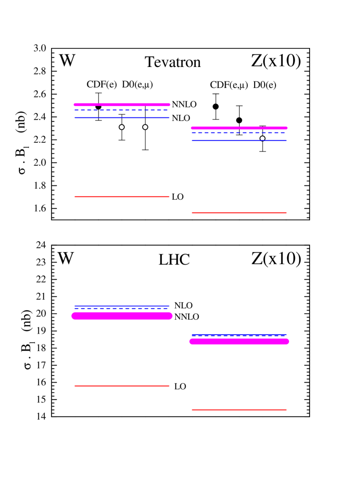
Figure 4: The predictions of the cross sections for $W$ and $Z$ production and leptonic decay at the Tevatron and the LHC obtained from parton sets of LO, NLO and NNLO global analyses of the same data set [26]. The cross sections labelled LO, NLO and NNLO are as in (4) and the dashed line is the NLO^′ prediction of (23). The band of the NNLO predictions allow for the ambiguity in the NNLO splitting functions [28]. Also shown are measurements obtained at the Tevatron [29, 30]. The figure is taken from [26].

Figure 5: The solid squares and triangles are the predictions of the NLO^′ cross sections of (23) for $W$ and $Z$ production and leptonic decay in $p\bar{p}$ collisions at $\sqrt{s}=1.8~{}{\rm TeV}$ obtained using various NLO sets of MRST99 partons [25]. The open square and small error bar are, respectively, the NLO and NNLO predictions of (4) using the MRST00 partons [26]. Also shown are the experimental measurements from CDF [29] and D0 [30]. For ease of reference $\pm 5\%$ lines are shown about the MRST99 default prediction. We thank W.J. Stirling for this figure, which combines results presented in [25, 26].

Figure 6: As for Fig. 5 but for $pp$ collisions at $\sqrt{s}=14~{}{\rm TeV}$.

Figure 7: Feynman diagrams driving $\gamma\gamma$ production in $pp$ collisions.

Figure 8: Contributions to the diphoton $p_{t}$ spectrum from the diagrams of Fig. 7 in $pp$ collisions at $\sqrt{s}=14~{}{\rm TeV}$. Each photon is required to have transverse momentum $p_{\gamma t}>20~{}{\rm GeV}$ and rapidity $|\eta_{\gamma}|<1$. The photons are required not to lie within the same $\eta-\phi$ cone of radius 0.4. We thank M.A. Kimber for this figure.

Figure 9: Higgs production via Pomeron-Pomeron fusion in $pp$ collisions.

References

- [1] ATLAS Collaboration: Detector and Physics Performance, Technical Design Report, CERN/LHCC/99-15 (1999).
- [2] F. Gianotti and M. Pepe-Altarelli, hep-ex/0006016.
- [3] ATLAS Collaboration: W.W. Armstrong et al., Technical Proposal, CERN Report CERN/LHCC/94-43 (1994).
- [4] CMS Collaboration: G.L. Bayatian et al., Technical Proposal, CERN Report CERN/LHCC/94-38 (1994).
- [5] CDF Collaboration: R. Blair et al., Technical Design Report, Nov. 1996, FERMILAB-PUB-96/390-E.
- [6] D0 Collaboration: (S. Abachi for collaboration), The D0 Upgrade: The Detector and its Physics, FERMILAB-PUB-96/357-E.
- [7] Del. Signore (for the CDF and D0 Collaborations), FERMILAB-Conf-98/221-E.
- [8] Totem Collaboration: M. Bozzo et al., Technical Proposal, CERN/LHCC/99-7.
- [9] V.M. Budnev, I.F. Ginzburg, G.V. Meledin and V.G. Serbo, Nucl. Phys. B63 (1973) 519.
- [10] K. Piotrzkowski, ‘Proposal for Luminosity Measurement at LHC’, ATLAS Internal Note ATL-PHYS-96-077 (1996).
-
[11]
A. Maslennikov, “Photon Physics in Novosibirsk”, Workshop on
Photon Interactions and Photon Structure, Lund (1998) 347;
A.G. Shamov and V.I. Telnov, ATLAS Note (in preparation). - [12] M. Dittmar, F. Pauss and D. Zürcher, Phys. Rev. D56 (1997) 7284.
-
[13]
H. Bethe, Ann. Phys. (N.Y.) 3 (1958) 190;
G.B. West and D.R. Yennie, Phys. Rev. 172 (1968) 1413. - [14] B.Z. Kopeliovich and A.V. Tarasov, hep-ph/0010062.
- [15] V.A. Khoze, A.D. Martin and M.G. Ryskin, hep-ph/0007359, Eur. Phys. J. (in press).
-
[16]
N. Kwak et al., Phys. Lett. B58 (1975) 233;
U. Amaldi et al., Phys. Lett. B66 (1977) 390;
L. Baksay et al., Nucl. Phys. B141 (1978) 1. - [17] A.A. Anselm and V.N. Gribov, Phys. Lett. B40 (1972) 487.
- [18] Particle Data Group, Eur. Phys. J. C15 (2000) 1.
-
[19]
V.M. Budnev, I.F. Ginzburg, G.V. Meledin and V.G. Serbo, Phys. Rep. 15 (1975) 181;
V.N. Baier, V.S. Fadin, V.A. Khoze and E.A. Kuraev, Phys. Rep. 78 (1981) 295. - [20] J. Pumplin, Phys. Rev. D52 (1995) 1477.
- [21] A. Berera and J.C. Collins, Nucl. Phys. B474 (1996) 183.
- [22] A.D. Martin, M.G. Ryskin and V.A. Khoze, Phys. Rev. D56 (1997) 5867.
- [23] K.A. Ispiryan, I.A. Nagorskaya, A.G. Oganesyan and V.A. Khoze, Sov. J. Nucl. Phys. 11 (1970) 712.
- [24] D.L. Borden, V.A. Khoze, W.J. Stirling and J. Ohnemus, Phys. Rev. D50 (1994) 4499.
- [25] A.D. Martin, R.G. Roberts, W.J. Stirling and R.S. Thorne, Eur. Phys. J. C14 (2000) 133.
- [26] A.D. Martin, R.G. Roberts, W.J. Stirling and R.S. Thorne, hep-ph/0007099, Eur. Phys. J (in press).
-
[27]
R. Hamburg, T. Matsuura and W.L. van Neerven, Nucl. Phys. B345
(1990) 331; B359 (1991) 343;
W.L. van Neerven and E.B. Zijlstra, Nucl. Phys. B382 (1992) 11. - [28] W.L. van Neerven and A. Vogt, Nucl. Phys. B568 (2000) 263; hep-ph/0005025; hep-ph/0006154.
-
[29]
CDF Collaboration: T. Affolder et al., Phys. Rev. Lett. 84 (2000)
845;
F. Abe et al., Phys. Rev. D59 (1999) 052002;
F. Abe et al., Phys. Rev. Lett. 76 (1996) 3070. -
[30]
D0 Collaboration: B. Abbott et al., Phys. Rev. D60 (1999) 052003;
J. Ellison, presentation at the EPS-HEP99 Conference, Tampere, Finland, July 1999. -
[31]
S. Catani, M. Ciafaloni and F. Hautmann, Phys. Lett. B242 (1990)
97; Nucl. Phys. B366 (1991) 135;
S. Catani and F. Hautmann, Nucl. Phys. B427 (1994) 475;
J.C. Collins and R.K. Ellis, Nucl. Phys. B360 (1991) 3. -
[32]
Yu.L. Dokshitzer, D.I. Dyakanov and S.I. Troyan, Phys. Rep. 58 (1980)
269;
M.A. Kimber, A.D. Martin and M.G. Ryskin, Eur. Phys. J. C12 (2000) 655. - [33] V.A. Khoze, A.D. Martin and M.G. Ryskin, Phys. Lett. B401 (1997) 330.
- [34] V.A. Khoze, A.D. Martin and M.G. Ryskin, Eur. Phys. J. C14 (2000) 525.
- [35] A.D. Martin, M.G. Ryskin and V.A. Khoze, Phys. Rev. D56 (1997) 5867.
- [36] A. Shuvaev, K. Golec-Biernat, A.D. Martin and M.G. Ryskin, Phys. Rev. D60 (1999) 014015.