$B_{K}$ in the chiral limit within the $1/N_{c}$ expansion.

Abstract

I report on a recent calculation done in collaboration with E. de Rafael [7] of the invariant $\hat{B}_{K}$ factor of $K^{0}$–$\bar{K^{0}}$ mixing in the chiral limit and to next–to– leading order in the $1/N_{c}$ expansion. This calculation is, to the best of our knowledge, the first example of a calculation of $\hat{B}_{K}$ in which there is an explicit analytic cancellation of the $\mu$ renormalization scale and the scheme dependence between the Wilson coefficient and the corresponding kaon matrix element. I try to emphasize the ideas involved in the approach and how the method could be applied to other physical situations, rather than the details of the numerical analysis for which I refer the reader to ref. [7].

1 INTRODUCTION

Real understanding of weak interactions of kaons is always hindered by the fact that their QCD interactions are not perturbative in $\alpha_{\mbox{\rm{\scriptsize s}}}$. This is a problem with (at least) two well separated scales (namely $M_{W}$ and $\Lambda_{QCD}\sim 1$ GeV) and, therefore, the well known technique of Effective Lagrangians can be applied. There is no problem as long as one is in the perturbative regime of the expansion in $\alpha_{\mbox{\rm{\scriptsize s}}}$, but kaons are lighter than $\Lambda_{QCD}$ and therefore this perturbative regime is long gone by the time one gets down to the kaon scale. In practice one assumes that the effective Lagrangian obtained after integrating the heavy fields of the Standard Model (i.e. heavier than $\Lambda_{QCD}$) is valid even immediately below the charm threshold. The problem then is to match this effective Lagrangian valid at $\mu{\ \lower-1.2pt\vbox{\hbox{\hbox to0.0pt{$<$\hss}\lower 5.0pt\vbox{\hbox{$\sim$}}}}\ }m_{c}$ to the effective Lagragian valid at $\mu\sim M_{K}$, wich is the relevant one.

To be more specific, integrating heavy fields in the Standard Model results in an effective $\Delta S=2$ Lagrangian that reads

$${{\cal L}}_{\rm eff}^{\Delta S=2}\!\!\!\!\!\! =\!\!\!\!\! -\frac{G_{F}^{2}M_{W}^{2}}{4\pi^{2}}\left[\lambda_{c}^{2}F_{1}+\lambda_{t}^{2}F_{2}+2\lambda_{c}\lambda_{t}F_{3}\right]$$ (1)

$$C_{\Delta S=2}(\mu)Q_{\Delta S=2}(x)\,,$$

where $\lambda_{q}=V_{\rm qd}^{\ast}V_{\rm qs}\,,\,{\rm q}={\rm u,c,t}\,,$ with $F_{1,2,3}$ being functions of the heavy masses of the fields $t$, $Z^{0}$, $W^{\pm}$, $b$, and $c$ which have been integrated out  and

$$Q_{\Delta S=2}(x)\equiv\big{[}\bar{s}_{L}(x)\gamma^{\mu}d_{L}(x)\big{]}^{2}\,,$$ (2)

with $q_{L}\equiv\frac{1-\gamma_{5}}{2}q$ is a four-quark operator. This four-quark operator has a hidden dependence on the renormalization scale because its matrix elements are divergent. This divergence is subtracted away using the ${\overline{MS}}$ renormalization scheme, but a $\mu$ scale dependence is left behind in the process. In fact, because the short distance behavior of the operator (2) is not the same as the matrix elements of the full Standard Model where $W$, etc.., are virtually propagating, one must introduce some coefficients, the so-called Wilson coefficients $C_{\Delta S=2}(\mu)$ that correct for this effect. It is a consistency condition then that the $\mu$ dependence should drop out of any physical observable, since after all one could always do the calculation in the full Standard Model (at least in principle), where no $\mu$ scale is necessary. Like with the $\mu$ parameter, the same “declaration of independence” also applies to any convention: naive dimensional regularization vs. ’t Hooft-Veltman, definition of evanescent operators, etc… However the question immediately arises, how can kaon matrix elements of the operator (2) know what you decided to do with the commutator of the $\gamma_{5}$ matrix in the calculation of $C_{\Delta S=2}(\mu)$ ? For one thing kaon matrix elements of the operator (2) will depend on masses and effective couplings but there can be no single Dirac matrix since kaons are bosons, of course! The dependence on conventions has to be implicitly hidden in what you call couplings and massess of mesons when you go away from d=4 dimensions in dimensional regularization. I shall explicitly demonstrate this point using the large-$N_{c}$ expansion later on. I shall also show the explict $\mu$ cancellation between Wilson coefficients and matrix elements of mesons.

At the scale $\mu\sim M_{K}$ chiral symmetry constraints the form of all the possible operators appearing in the correspondimng effective Lagrangian in a chiral expansion in powers of derivatives and masses. To lowest order, which is ${\cal O}(p^{2})$, there is a unique operator with the same symmetry properties as $Q_{\Delta S=2}(x)$, which is [3, 4]

$$-\frac{F_{0}^{4}}{4}\ g_{\Delta S=2}(\mu)\ \mbox{\rm tr}\left[\lambda_{32}(D^{\mu}U^{\dagger})U\lambda_{32}(D_{\mu}U^{\dagger})U\right]\,,$$ (3)

where $\lambda_{32}$ and $U$ are matrices in flavor space. $\lambda_{32}$ denotes the matrix $\lambda_{32}=\delta_{i3}\delta_{2j}$, and $U$ is the $3\times 3$ unitary matrix which collects the Goldstone fields and which under chiral rotations transforms like $U\rightarrow V_{R}UV_{L}^{\dagger}$. The parameter $g_{\Delta S=2}(\mu)$ is a dimensionless coupling constant which depends on the underlying dynamics of spontaneous chiral symmetry breaking (S$\chi$SB) in QCD and that has to be determined, as always, by a matching condition. Leaving aside the known functions $F_{1,2,3}$ it has become conventional to define the so-called invariant $\hat{B}_{K}$ parameter by means of the following matrix element

$$<\bar{K}^{0}|C_{\Delta S=2}(\mu)Q_{\Delta S=2}(0)|K^{0}>\equiv\frac{4}{3}f_{K}^{2}M_{K}^{2}\hat{B}_{K}.$$ (4)

Because of the presence of $C_{\Delta S=2}(\mu)$, $\hat{B}_{K}$ so defined must be $\mu$ (and convention) independent. There is also an analogous equation without the wilson coefficient $C_{\Delta S=2}(\mu)$ that defines the associated $B_{K}(\mu)$ parameter which, unlike $\hat{B}_{K}$, is obviously $\mu$ (and convention) dependent. From Eqs. (4,3) it follows that (with inclusion of the chiral corrections in the factorized contribution)

$$\hat{B}_{K}=\frac{3}{4}C_{\Delta S=2}(\mu)\times g_{\Delta S=2}(\mu)\,,$$ (5)

in other words, $\hat{B}_{K}$ is also fixed by a matching condition. The rest of this paper is a report on the calculation of $\hat{B}_{K}$ carried out in ref. [7].

The Wilson coefficient is known from renormalization group-improved perturbation theory and reads

$$C_{\Delta S=2}(\mu)=$$

$$\!\!\!\!\left[1+\frac{\alpha_{\mbox{\rm{\scriptsize s}}}(\mu)}{\pi}\frac{1}{\beta_{1}}\left(\gamma_{2}+\frac{\gamma_{1}}{-\beta_{1}}\beta_{2}\right)\right]\left(\frac{1}{\alpha_{\mbox{\rm{\scriptsize s}}}(\mu)}\right)^{\frac{\gamma_{1}}{-\beta_{1}}}\,$$ (6)

$$\!\!\!\!\rightarrow\!\left[1+\frac{\alpha_{\mbox{\rm{\scriptsize s}}}(\mu)}{\pi}\left(\frac{1433}{1936}+\frac{1}{8}\kappa\right)\right]\left(\frac{1}{\alpha_{\mbox{\rm{\scriptsize s}}}(\mu)}\right)^{\frac{9}{11}\frac{1}{N_{c}}}\,,$$ (7)

where the explicit expressions for $\beta_{1},\beta_{2},\gamma_{1}$ and $\gamma_{2}$ can be found in ref.[7] and $\kappa$ encodes the choices for $\gamma_{5}$ in d dimensions: $\kappa=0$ in naive dimensional regularization and $\kappa=-4$ in the ’t Hooft-Veltman scheme. Eq. (7) is obtained after insisting on the large-$N_{c}$ limit, which consists in taking $N_{c}\rightarrow\infty$ with the condition $N_{c}\alpha_{\mbox{\rm{\scriptsize s}}}\rightarrow constant$[5]. In the strict large-$N_{c}$ limit one finds

$$\hat{B}_{K}=\frac{3}{4}\quad,\quad(N_{c}\rightarrow\infty)\ .$$ (8)

As to the large-$N_{c}$ expansion, reference [6] explains why taking this limit is a useful thing to do because it simplifies QCD without crippling it; although the assumption that QCD confines in this limit must be made.

For us it will be very important that, because the large-$N_{c}$ expansion is a systematic approximation to QCD (both in the perturbative and nonperturbative regimes), it can be used as an interpolating function between low energies and high energies in a systematic way.

Our calculation will be based on the following inputs:

• The large $N_{c}$ expansion.

• Chiral perturbation theory controls the low-energy end of QCD Green’s functions.

• The Operator Product Expansion controls the high-energy end of QCD Green’s functions starting from $Q\sim 1$GeV onwards.

• The curve connecting low-energy and high-energy is smooth, i.e. there are no “wiggles” in the intermediate region. Such wiggles would destroy the cherished belief that Nature seems to be “subtle but not malicious”.

Let us now go on with the matching condition that $g_{\Delta S=2}(\mu)$ must satisfy. From the fact that the covariant derivatives contain external fields ($D^{\mu}U^{\dagger}U=\partial^{\mu}U^{\dagger}U+iU^{\dagger}r^{\mu}U-il^{\mu}$), one sees that Eq. (3) yields a mass term for the external $r^{\mu}_{\bar{d}s}$ field, among other terms. This $r^{\mu}_{\bar{d}s}$ is of course the same external field that couples to the right-handed current $\bar{d}_{R}\gamma^{\mu}s_{R}$ appearing in the kinetic term for the quark in QCD, i.e.

$$\bar{q}\!\!\left\{\gamma^{\mu}(\partial_{\mu}\!\!+iG_{\mu})\!\!-\!i\gamma^{\mu}\!\left[l_{\mu}\frac{1-\gamma_{5}}{2}\!+\!r_{\mu}\frac{1+\gamma_{5}}{2}\!\right]\!\right\}q\,.$$ (9)

Therefore at the level of the QCD Lagrangian a mass term for the $r^{\mu}_{\bar{d}s}$ field can only come about because of the operator $Q_{\Delta S=2}$ of Eq. (2) in the Lagrangian (1). Equating the mass term $r^{\mu}_{\bar{d}s}r_{\mu}^{\bar{d}s}$ obtained from Eq. (3) to that obtained from Eq. (1) (supplemented with ${\cal L}_{\rm QCD}$ of course) one obtains the matching condition for $g_{\Delta S=2}(\mu)$[7]:

$$g_{\Delta S=2}(\mu,\epsilon)=\quad 1-$$

$$\frac{\mu_{\mbox{\rm{\scriptsize had.}}}^{2}}{32\pi^{2}F_{0}^{2}}\ \frac{(4\pi\mu^{2}/\mu_{\mbox{\rm{\scriptsize had.}}}^{2})^{\epsilon/2}}{\Gamma(2-\epsilon/2)}\!\!\int_{0}^{\infty}\!\!\!\!\!\!\!dz\ z^{-\epsilon/2}W(z)\,,$$ (10)

where $\mu_{\mbox{\rm{\scriptsize had.}}}^{2}$ is a scale used for normalization, e.g. $z\equiv Q^{2}/\mu_{\mbox{\rm{\scriptsize had.}}}^{2}$, but otherwise totally arbitrary. Therefore the apparent quadratic dependence of Eq. (1) on $\mu_{\mbox{\rm{\scriptsize had.}}}$ is actually fictitious. There will be nevertheless a certain $\mu_{\mbox{\rm{\scriptsize had.}}}$ dependence in the final answer for $\hat{B}_{K}$ due to the fact that there is always a residual $\mu$ dependence because the effective Lagrangian of Eq. (1) is constructed only to next-to-leading order in $\alpha_{\mbox{\rm{\scriptsize s}}}$ (see Eqs.(6,7)) and we will identify $\mu=\mu_{\mbox{\rm{\scriptsize had.}}}$ as a typical hadronic scale. For the final numerical applications we shall take $1\,\mbox{\rm GeV}\leq\mu_{\mbox{\rm{\scriptsize had.}}}\leq 3\,\mbox{\rm GeV}$.

The divergent (i.e. ill-defined) integral defining $g_{\Delta S=2}(\mu,\epsilon)$ in Eq. (1) must be understood within the same regularization procedure and conventions used to compute $C_{\Delta S=2}(\mu)$ in Eq. (7), i.e. ${\overline{MS}}$ and the definition of evanescent operators of ref. [8].

The function $W(z)$ is defined as

$$W(z)=z\frac{\mu_{\mbox{\rm{\scriptsize had.}}}^{2}}{F_{0}^{2}}{\cal W}^{(1)}_{LRLR}(z\mu_{\mbox{\rm{\scriptsize had.}}}^{2})\ ,$$ (11)

where ${\cal W}^{(1)}_{LRLR}$ is defined through an integral over the solid angle of the momentum $q$,

$$\int d\Omega_{q}\ g_{\mu\nu}{\cal W}_{LRLR}^{\mu\alpha\nu\beta}(q,l)|_{\mbox{\rm{\scriptsize unfactorized}}}=$$

$$\qquad\left(\frac{l^{\alpha}l^{\beta}}{l^{2}}-g^{\alpha\beta}\right)\ {\cal W}^{(1)}_{LRLR}(Q^{2})\,,$$ (12)

and $Q^{2}\equiv-q^{2}$. In Eq. (1) the function ${\cal W}_{LRLR}^{\mu\alpha\nu\beta}(q,l)$ stands for

$${\cal W}_{LRLR}^{\mu\alpha\nu\beta}(q,l)=i^{3}\lim_{l\rightarrow 0}\!\int\!\!d^{4}xd^{4}yd^{4}z\ e^{i(q\cdot x+l\cdot y-l\cdot z)}$$

$$\langle 0|T\{L_{\bar{s}d}^{\mu}(x)\ R_{\bar{d}s}^{\alpha}(y)\ L_{\bar{s}d}^{\nu}(0)\ R_{\bar{d}s}^{\beta}(z)\}|0\rangle\quad,$$ (13)

with

$$L_{\bar{s}d}^{\mu}(x)=\bar{s}(x)\gamma^{\mu}\frac{1-\gamma_{5}}{2}d(x)\ ,$$ (14)

and

$$R_{\bar{d}s}^{\mu}(x)=\bar{d}(x)\gamma^{\mu}\frac{1+\gamma_{5}}{2}s(x)\ .$$ (15)

Since $W(z)\sim{\cal O}(N_{c}^{0})$ and $F_{0}^{2}\sim{\cal O}(N_{c})$ one sees that Eq. (1) yields $g_{\Delta S=2}(\mu,\epsilon)=1-{\cal O}(1/N_{c})$ with the subleading term governed by $W(z)$.

What do we know about $W(z)$ ? In general $W(z)$ is a complicated function of the variable $z$. However in the large-$N_{c}$ limit it simplifies somewhat and can be expressed as an infinite sum of single, double and triple poles in the form

$$W[z]=6-\sum_{i=1}^{\infty}\frac{\alpha_{i}}{\rho_{i}}-\sum_{i=1}^{\infty}\frac{\beta_{i}}{\rho_{i}^{2}}$$

$$+\sum_{i=1}^{\infty}\left\{\frac{\alpha_{i}}{(z+\rho_{i})}+\frac{\beta_{i}}{(z+\rho_{i})^{2}}+\frac{\gamma_{i}}{(z+\rho_{i})^{3}}\right\},$$ (16)

where $\rho_{i}=M_{i}^{2}/\mu_{\mbox{\rm{\scriptsize had.}}}^{2}$ and $M_{i}$ is the mass of the $i$–th zero-width resonance. If one knew all the masses and constants appearing in $W(z)$ from the solution to large-$N_{c}$ QCD one could use this information, plug it in Eq. (1) and compute $\hat{B}_{K}$ through Eq. (5). Since this solution is not available, we will have to follow a different strategy. Firstly, one recalls that it is due to the presence of a perturbative contribution to a given Green’s function that one must take these sums over resonances truly up to infinity because otherwise parton-model logarithms cannot be reproduced[6]. Clearly, when the sums extend all the way to infinity, in general one cannot expand in powers of $1/z$ at large $z$ in a naive way. However our function $W(z)$ is an order parameter of spontaneous chiral symmetry breaking or, in other words, the contribution of perturbation theory to $W(z)$ vanishes to all orders. One can then try to match a naive expansion in $1/z$ to the Operator Product Expansion considering finite sums as an approximation to the originally infinite sums. This way one can fix the unknown parameters and masses through the knowledge on the behavior of $W(z)$ at large $z$ given by this Operator Product Expansion.

We have no proof that these infinite sums have to behave as if they were finite but we know that, if this is so, a successful framework such as Vector Meson Dominance then becomes the leading term in the approximation to large $N_{c}$ that we propose, instead of a phenomenological ansatz[9]. Besides, our approximation works well in those cases where we can compare with the experiment[10, 11].

Consequently we impose the following behavior on $W(z)$:

• i)At low $z$, from chiral perturbation theory, one finds [12, 13, 14, 7]

  $$W(z)\approx\quad 6$$

  $$-24\frac{\mu_{\mbox{\rm{\scriptsize had.}}}^{2}}{F_{0}^{2}}\left(2L_{1}+5L_{2}+L_{3}+L_{9}\right)\ z$$

  $$\qquad\qquad+\dots$$

• ii)At high $z$, from the operator product expansion, one gets[7]

  $$W(z)\approx$$

  $$\frac{24\pi\alpha_{\mbox{\rm{\scriptsize s}}}F_{0}^{2}}{\mu_{\mbox{\rm{\scriptsize had.}}}^{2}}\left[1\!\!+\!\frac{\epsilon}{12}\left(5\!+\kappa\right)\!+{\cal O}(\alpha_{\mbox{\rm{\scriptsize s}}})\right]\frac{1}{z}$$

  $$\qquad\qquad+\dots$$ (18)

Notice that in i) chiral logarithms are neglected, in accord with the large-$N_{c}$ expansion. It is a phenomenological fact that they are small in vector and axial-vector channels, which are precisely the relevant ones here. For the $L_{i}$ couplings we use lowest meson dominance, as explained in ref. [10, 9]. This also works phenomenologically. The factor of 6 in Eq. (• ‣ 1) explains the corresponding factor in $W(z)$ in Eq. (1).

As to ii), notice the $\epsilon$ and $\kappa$ dependence of the result. This is brought about by the need to do the calculation in d dimensions, as repeatedly emphasized. Then the appearance of structures like $\gamma_{\lambda}(1-\gamma_{5})\gamma_{\rho}\gamma_{\mu}\otimes\gamma^{\lambda}(1-\gamma_{5})\gamma^{\rho}\gamma^{\mu}$ in the OPE calculation of $W(z)$ makes the definition of $\gamma_{5}$ and evanescent operators of practical relevance. We followed closely refs. [8, 2].

Considering the higher orders in Eq. (• ‣ 1) there has recently been the warning, issued by the authors of ref. [15], that these subleading effects in the OPE expansion might actually be numerically important. I don’t expect this to be the case here because, as we shall see, the impact of the OPE fall-off in the final numerical value is not large, but a more detailed analysis is currently underway[16].

All in all, Eqs.(• ‣ 1,• ‣ 1) impose the following conditions on the parameters and masses of $W(z)$:

$$\sum_{i=1}^{\infty}\frac{\alpha_{i}}{\rho_{i}^{2}}+2\sum_{i=1}^{\infty}\frac{\beta_{i}}{\rho_{i}^{3}}+3\sum_{i=1}^{\infty}\frac{\gamma_{i}}{\rho_{i}^{4}}=$$

$$24\frac{\mu_{\mbox{\rm{\scriptsize had.}}}^{2}}{F_{0}^{2}}[2L_{1}+5L_{2}+L_{3}+L_{9}]\,$$ (19)

from ${\cal O}(z)$ terms in Eq. (• ‣ 1). Furthermore,

$$\sum_{i=1}^{\infty}\frac{\alpha_{i}}{\rho_{i}}+\sum_{i=1}^{\infty}\frac{\beta_{i}}{\rho_{i}^{2}}+\sum_{i=1}^{\infty}\frac{\gamma_{i}}{\rho_{i}^{3}}=6\,$$ (20)

from the absence of ${\cal O}(1/z^{0})$ terms in Eq. (• ‣ 1); also

$$\sum_{i=1}^{\infty}\alpha_{i}={\cal R}+\frac{\epsilon}{2}{\cal S}\,,$$ (21)

with

$${\cal R}=\left[24\pi^{2}\frac{\alpha_{\mbox{\rm{\scriptsize s}}}}{\pi}+{\cal O}\left(\frac{N_{c}\alpha_{\mbox{\rm{\scriptsize s}}}^{2}}{\pi^{2}}\right)\right]\frac{F_{0}^{2}}{\mu_{\mbox{\rm{\scriptsize had.}}}^{2}}\quad$$

$${\cal S}=\left[4\pi^{2}(5+\kappa)\frac{\alpha_{\mbox{\rm{\scriptsize s}}}}{\pi}+{\cal O}\left(\frac{N_{c}\alpha_{\mbox{\rm{\scriptsize s}}}^{2}}{\pi^{2}}\right)\right]\frac{F_{0}^{2}}{\mu_{\mbox{\rm{\scriptsize had.}}}^{2}}\quad,$$ (22)

from the ${\cal O}(1/z)$ term in Eq. (• ‣ 1).

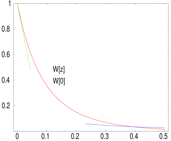
Figure 1: Plot of the hadronic function $W[z]$ in Eq. (1) versus $z=Q^{2}/\mu_{\mbox{\rm{\scriptsize had.}}}^{2}$ for $\mu_{\mbox{\rm{\scriptsize had.}}}=1.4$ GeV, $F_{0}=85.3$ MeV and $M_{V}=770$ MeV. The red curve is the function $W[z]$ corresponding to the contribution of a single $\rho$ resonance (see text). The green line represents the low–energy chiral behaviour and the blue curve the prediction from the OPE.

When all these constraints are imposed on $W(z)$ in Eq. (1) the expression for $g_{\Delta S=2}(\mu)$ in Eq. (1) in the ${\overline{MS}}$ renormalization scheme reads

$$g_{\Delta S=2}^{(r)}(\mu)=1-\frac{\mu_{\mbox{\rm{\scriptsize had.}}}^{2}}{32\pi^{2}F_{0}^{2}}\Bigg{\{}{\cal R}\log\frac{\mu^{2}}{\mu_{\mbox{\rm{\scriptsize had.}}}^{2}}+\!\!{\cal R}\!+\!\!{\cal S}$$ (23)

$$\quad\quad+\sum_{i=1}^{\infty}\left[-\alpha_{i}\log\rho_{i}+\frac{\beta_{i}}{\rho_{i}}+\frac{1}{2}\frac{\gamma_{i}}{\rho_{i}^{2}}\right]\Bigg{\}}\ ,$$

$$\Rightarrow \left(\frac{\alpha_{\mbox{\rm{\scriptsize s}}}(\mu)}{\alpha_{\mbox{\rm{\scriptsize s}}}(\mu_{\mbox{\rm{\scriptsize had.}}})}\right)^{\frac{9}{11}\frac{1}{N_{c}}}\!\!\Bigg{\{}1-\frac{1}{2}\frac{\mu_{\mbox{\rm{\scriptsize had.}}}^{2}}{16\pi^{2}F_{0}^{2}}\Bigg{(}\!{\cal R}\!+\!{\cal S}\!$$

$$\quad\quad+\sum_{i=1}^{\infty}\left[-\alpha_{i}\log\rho_{i}+\frac{\beta_{i}}{\rho_{i}}+\frac{1}{2}\frac{\gamma_{i}}{\rho_{i}^{2}}\right]\Bigg{)}\Bigg{\}}\,,$$

where in the second line we have written the renormalization group-improved result. We would like to insist on the fact that this result, contrary to the various large–$N_{c}$ inspired calculations which have been published so far [17, 18, 3, 12, 19, 13, 14] is the full result to next–to–leading order in the $1/N_{c}$ expansion. The renormalization $\mu$ scale dependence as well as the scheme dependence in the factor ${\cal S}$ cancel exactly, at the next–to–leading log approximation, with the short distance $\mu$ and scheme dependences in the Wilson coefficient $C_{\Delta S=2}(\mu)$ in Eq. (7). Therefore, the full expression of the invariant $\hat{B}_{K}$–factor to lowest order in the chiral expansion and to next–to–leading order in the $1/N_{c}$ expansion, which takes into account the hadronic contribution from light quarks below a mass scale $\mu_{\mbox{\rm{\scriptsize had.}}}$ is then

$$\hat{B}_{K}=\left(\frac{1}{\alpha_{\mbox{\rm{\scriptsize s}}}(\mu_{\mbox{\rm{\scriptsize had.}}})}\right)^{\frac{3}{11}}\frac{3}{4}$$

$$\left\{1-\frac{\alpha_{\mbox{\rm{\scriptsize s}}}(\mu_{\mbox{\rm{\scriptsize had.}}})}{\pi}\frac{1229}{1936}+{\cal O}\left(\frac{N_{c}\alpha_{\mbox{\rm{\scriptsize s}}}^{2}}{\pi^{2}}\right)\right.$$

$$-\left.\frac{\mu_{\mbox{\rm{\scriptsize had.}}}^{2}}{32\pi^{2}F_{0}^{2}}\sum_{i=1}^{\infty}\left[-\alpha_{i}\log\rho_{i}+\frac{\beta_{i}}{\rho_{i}}+\frac{1}{2}\frac{\gamma_{i}}{\rho_{i}^{2}}\right]\right\}\,.$$ (24)

As remarked earlier, the numerical choice of the hadronic scale $\mu_{\mbox{\rm{\scriptsize had.}}}$ is, a priori, arbitrary. In practice, however, $\mu_{\mbox{\rm{\scriptsize had.}}}$ has to be sufficiently large so as to make meaningful the truncated pQCD series in the first line. Our final error in the numerical evaluation of $\hat{B}_{K}$ will include the small effect of fixing $\mu_{\mbox{\rm{\scriptsize had.}}}$ within the range $1\,\mbox{\rm GeV}\leq\mu_{\mbox{\rm{\scriptsize had.}}}\leq 3\,\mbox{\rm GeV}$.

How many resonances should one include in the sum in Eq. (1)? Clearly, the more the better. However, given that there is only a limited amount of information coming from Eqs. (• ‣ 1, • ‣ 1) one can in practice determine the couplings of just one resonance, the $\rho$ vector meson. With them, and given the rho mass, the corresponding $W(z)$ function of Eq. (1) is shown in Fig. 1, where it is seen that $W(z)$ intersects the OPE curve at a certain value of $z$ that we will call $\hat{z}$. It turns out that $\hat{z}\sim 0.39$ (i.e. $Q\sim 900$ MeV). As can be seen, the matching to the OPE curve is not perfect and this is why, for the final numerical estimate, we propose to use the hadronic curve $W(z)$ only in the region $0\leq z\leq\hat{z}$ while in the range $\hat{z}\leq z<\infty$ we use the first term of the OPE, Eq. (• ‣ 1). This results in a different expression for the $\hat{B}_{K}$ parameter which reads

$$\hat{B}_{K}\left(\rho,a_{1},\rho^{\prime}\right)=\left(\frac{1}{\alpha_{\mbox{\rm{\scriptsize s}}}(\mu_{\mbox{\rm{\scriptsize had.}}})}\right)^{\frac{3}{11}}\frac{3}{4}$$

$$\Bigg{\{}\!1\!\!-\!\frac{\alpha_{\mbox{\rm{\scriptsize s}}}(\mu_{\mbox{\rm{\scriptsize had.}}})}{\pi}\left[\frac{1229}{1936}-\!\frac{3}{4}\!\log\hat{z}\right]\!+\!{\cal O}\left(\frac{N_{c}\alpha_{\mbox{\rm{\scriptsize s}}}^{2}}{\pi^{2}}\right)$$

$$-\frac{\mu_{\mbox{\rm{\scriptsize had.}}}^{2}}{32\pi^{2}F_{0}^{2}}\!\!\Big{[}\alpha_{V}\log\frac{\hat{z}+\rho_{V}}{\rho_{V}}-\beta_{V}\left(\frac{1}{\hat{z}+\rho_{V}}-\frac{1}{\rho_{V}}\right)$$

$$-\frac{\gamma_{V}}{2}\left(\frac{1}{(\hat{z}+\rho_{V})^{2}}-\frac{1}{\rho_{V}^{2}}\right)\Big{]}\Bigg{\}}\,.$$ (25)

Of course in the limit $\hat{z}\rightarrow\infty$, Eq. (1) reproduces Eq.(1), but this limit in practice can only be achieved by using more and more resonances in the sum, which requires the knowledge of more and more terms in both the low and high-energy expansions of $W(z)$. The physical interpretation of the result (1) is clear: the area under the curve in Fig. 1 is roughly the amount one subtracts from the large-$N_{c}$ limit result of $\hat{B}_{K}=3/4$. In numbers one gets

$$\hat{B}_{K}=0.38\pm 0.11\,,$$ (26)

where the error is the combined limit of errors from short– (e.g. how much is $\Lambda_{\overline{MS}}$?) and long–distance (e.g. how much is the $\rho$ mass?) contributions to $\hat{B}_{K}$ for a choice of $\mu_{\mbox{\rm{\scriptsize had.}}}$ in the range $1\,\mbox{\rm GeV}\leq\mu_{\mbox{\rm{\scriptsize had.}}}\leq 3\,\mbox{\rm GeV}$. I refer the reader to ref. [7] for details. This result, of course, does not include the error due to next–to–next–to leading terms in the $1/N_{c}$ expansion, nor the error due to chiral corrections in the unfactorized contribution, but we consider it to be a rather robust prediction of $\hat{B}_{K}$ in the chiral limit and at the next–to– leading order in the $1/N_{c}$ expansion for the following reasons. Firstly, Fig. 1 shows that most of the area under the curve is in the region $0\leq z{\ \lower-1.2pt\vbox{\hbox{\hbox to0.0pt{$<$\hss}\lower 5.0pt\vbox{\hbox{$\sim$}}}}\ }0.4$ which makes the final number for $\hat{B}_{K}$ relatively insensitive to the part of the curve coming from the OPE. Secondly, at a more qualitative level, if one accepts that the low-$z$ region is correctly given by Chiral Perturbation Theory up to a scale of $z\sim 0.06$ (i.e. $E\sim 350$ MeV) and the OPE also describes reasonably well the high-$z$ region starting from $z\sim 0.5$ ($E\sim 1$ GeV); then the conclusion is that there isn’t much room left in between to do a lot of things !

Our final result in Eq.( 26) is compatible with the current algebra prediction [20] obtained from the $K^{+}\rightarrow\pi^{+}\pi^{0}$ decay rate at lowest order in chiral perturbation theory. It turns out [21] that the bosonization of the four–quark operator $Q_{\Delta S=2}$ and the bosonization of the operator $Q_{2}-Q_{1}$ which generates $\Delta I=1/2$ transitions are related to each other in the combined chiral limit and next–to–leading order $1/N_{c}$ expansion. It follows that decreasing the value of $\hat{B}_{K}$ from the large–$N_{c}$ prediction of 3/4 down to the result in Eq. (26) is correlated with an increase of the coupling constant in the lowest order Effective Chiral Lagrangian which generates $\Delta I=1/2$ transitions, providing therefore a first glimpse at a quantitative understanding of the dynamical origin of the $\Delta I=1/2$ rule. In the future we would like to make some refinements and a detailed comparison between our result and other previous estimates[16]. Among these “refinements” one has most notably the inclusion of higher order terms in the chiral expansion. These are crucial in order to be able to make a meaningful comparison with the values favoured by lattice QCD determinations [22] as well as by recent phenomenological analysis [23, 24].

I would not like to finish without stressing that our framework can in principle be improved systematically, for instance by computing more terms in Eqs. (• ‣ 1,• ‣ 1). It can be applied as well to other physical situations involving weak matrix elements. In order to do this one might find helpful the following

DO-IT-YOURSELF KIT:

• i)Pick the QCD Green’s function, ${\cal G}$, which defines the matrix element you are interested in.

• ii)Find the large-$N_{c}$ resonance representation of ${\cal G}$ (i.e. the interpolating function).

• iii)Impose on the above interpolating function the long- and short-distance constraints stemming from Chiral Perturbation Theory and the Operator Product Expansion, respectively.

• iv)Compute number.

• v)Enjoy.

Acknowledgments

I thank E. de Rafael for a most enjoyable collaboration. During the elaboration of this work we benefited a great deal from discussions with Marc Knecht. We also thank Hans Bijnens, Maarten Golterman, Michel Perrottet, Toni Pich and Ximo Prades for discussions. (S.P.) is also grateful to C. Bernard and Y. Kuramashi for conversations and to the Physics Dept. of Washington University in Saint Louis for the hospitality extended to him while the work of ref. [7] was being finished. This work has been supported in part by TMR, EC-Contract No. ERBFMRX-CT980169 (EURODA$\phi$NE) and by the research project CICYT-AEN99-0766. I thank S. Narison for his kind invitation to the Conference.

DISCUSSION

H. Fritzsch (Munich)

I would expect that you encountered problems with your technique if the singlet $0^{-+}$ is involved since the role of the gluon anomaly is different for large $N_{c}$.

S.P.

As is well known, the gluon anomaly is at the origin of the $\eta^{\prime}$ mass. In the strict large $N_{c}$ limit the anomaly is switched off and $M_{\eta^{\prime}}\rightarrow 0$. It may seem then that the large-$N_{c}$ expansion is a very bad expansion for the $\eta^{\prime}$ since in the real world $M_{\eta^{\prime}}\sim M_{\rm proton}\sim 1$ GeV $>>M_{\pi}$; i.e. it doesn’t look at all like a Goldstone boson which is what the $N_{c}=\infty$ result says.

Although I don’t know whether the $1/N_{c}$ expansion will be in the end really helpful for calculations involving the $0^{-+}$ channel, I would like to explain why I think that the above argument is potentially fallacious. Take good old QED as an expansion in powers of $\alpha$ around $\alpha=0$. If you were to compare the real world (where e^- and e⁺ certainly scatter) to what you find from the strictly speaking first term in this expansion , which is the one at $\alpha=0$ (i.e. no scattering), you could also conclude that the $\alpha$ expansion is a disaster. Well, in some respects $\alpha=0$ corresponds to $N_{c}=\infty$. In other words, one should always go to first nontrivial order in the expansion before comparing to the real world. It is not unconceivable then that, after the bulk of the $\eta^{\prime}$ mass is included in the first nontrivial term in the $1/N_{c}$ expansion, the rest of the series in $1/N_{c}$ turns out to be a well-behaved innocent-looking power series.

Having said this, I also want to stress that in our particular case of $\hat{B}_{K}$, at the order we are computing, the $0^{-+}$ channel doesn’t play any role at all. It’s all governed by vectors and axial-vectors for which we know that resonance saturation (which is basically what the large-$N_{c}$ expansion amounts to in this case) is a good thing to do. (I thank M. Knecht for reminding me of this.)

References

- [1] A.J. Buras, M. Jamin and P. Weisz, Nucl. Phys. B347 (1990) 491; S. Herrlich and U. Nierste, Nucl. Phys. B419 (1994) 292, ibid. Nucl. Phys. B476 (1996) 27.
- [2] G. Buchalla, A.J. Buras and M.E. Lautenbacher, Rev. Mod. Phys. 68 (1996) 1125; A.J. Buras, in Les Houches Lectures, Session LXVIII, Probing the Standard Model of Particle Interactions, eds. R. Gupta, A. Morel, E. de Rafael and F. David, North–Holland 1999.
- [3] A. Pich and E. de Rafael, Nucl. Phys. B358 (1991) 311.
- [4] E. de Rafael, “Chiral Lagrangians and Kaon CP–Violation”, in CP Violation and the Limits of the Standard Model, Proc. TASI’94, ed. J.F. Donoghue (World Scientific, Singapore, 1995)
- [5] G ’t Hooft, Nucl. Phys. B72 (1974) 461; B75 (1974) 461.
- [6] E. Witten, Nucl. Phys. B79 (1979) 57.
- [7] S. Peris and E. de Rafael, Phys. Lett. B490 (2000) 213. A missing term in the function of this reference has been corrected in hep-ph/0006146 v3.
- [8] A.J. Buras and P.H. Weisz, Nucl. Phys. B333 (1990) 66.
- [9] M. Knecht, S. Peris and E. de Rafael, Nucl. Phys. (Proc. Suppl.) B86 (2000) 279; see also M. Knecht and E. de Rafael, Phys. Lett. B424 (1998) 335; S. Peris, M. Perrottet and E. de Rafael, JHEP 05 (1998) 011; M. Golterman and S. Peris, Phys. Rev.D61 (2000) 034018.
- [10] G. Ecker, J. Gasser, A. Pich and E. de Rafael, Nucl. Phys. B321 (1989) 311; G. Ecker, J. Gasser, H. Leutwyler, A. Pich and E. de Rafael, Phys. Lett. B223 (1989) 425.
- [11] S. Peris, B. Phily and E. de Rafael, hep-ph/0007338; M. Knecht, S. Peris, M. Perrottet and E. de Rafael, Phys. Rev. Lett. 83 (1999) 5230; see also M. Kecht, S. Peris and E. de Rafael, Phys. Lett. B443 (1998) 255.
- [12] J.P. Fatelo and J.-M. Gèrard, Phys. Lett. B347 (1995) 136.
- [13] T. Hambye, G.O. Köhler and P.H. Soldan, Eur. Phys. J. C10 (1999) 271.
- [14] J. Bijnens and J. Prades, Phys. Lett. JHEP 01 (1999) 023.
- [15] V. Cirigliano, J.F. Donoghue and E. Golowich, hep-ph/0007196; J.F. Donoghue, these proceedings.
- [16] S. Peris and E. de Rafael, in preparation.
- [17] W.A. Bardeen, A.J. Buras and J.-M. Gèrard, Phys. Lett. B211 (1988) 343.
- [18] J.-M. Gèrard, Acta Physica Polonica B21 (1990) 257.
- [19] S. Bertolini, J.O. Egg, M. Fabbrichesi and E.I. Lashin, Nucl. Phys. B514 (1998) 63.
- [20] J.F. Donoghue, E. Golowich and B.R. Holstein, Phys. Lett. B119 (1982) 412.
- [21] A. Pich and E. de Rafael, Phys. Lett. B374 (1996) 186.
- [22] Y. Kuramashi, Nucl. Phys. B (Proc. Suppl.) 83-84 (2000) 24.
- [23] M. Ciuchini, E. Franco, L. Giusti, V. Lubicz, G. Martinelli, Nucl. Phys. B573 (2000) 201.
- [24] F. Caravaglios, F. Parodi, P. Roudeau and A. Stocchi, hep-ph/0002171.