hep-ph/0010081 CERN-TH/2000-206

 

 

Measuring the SUSY Breaking Scale at the LHC

in the Slepton NLSP Scenario of GMSB Models${}^{\>\star}$

S. Ambrosanio ^a, B. Mele ^b,c, S. Petrarca ^c,b, G. Polesello ^d, A. Rimoldi ^e,f

^a CERN, Theory Division, CH–1211 Geneva 23, Switzerland
 
^b INFN, Sezione di Roma I, Roma, Italy
 
^c Dipartimento di Fisica, Università “La Sapienza”,
p.le Aldo Moro 2, I–00185 Roma, Italy
 
^d INFN, Sezione di Pavia, via Bassi 6, I–27100 Pavia, Italy
 
^e CERN, EP Division, CH–1211 Geneva 23, Switzerland
 
^f Dipartimento di Fisica Nucleare e Teorica, Università di Pavia,
via Bassi 6, I–27100 Pavia, Italy

Abstract

We report a study on the measurement of the SUSY breaking scale $\sqrt{F}$ in the framework of gauge-mediated supersymmetry breaking (GMSB) models at the LHC. The work is focused on the GMSB scenario where a stau is the next-to-lightest SUSY particle (NLSP) and decays into a gravitino with lifetime $c\tau_{\rm NLSP}$ in the range 0.5 m to 1 km. We study the identification of long-lived sleptons using the momentum and time of flight measurements in the muon chambers of the ATLAS experiment. A realistic evaluation of the statistical and systematic uncertainties on the measurement of the slepton mass and lifetime is performed, based on a detailed simulation of the detector response. Accessible range and precision on $\sqrt{F}$ achievable with a counting method are assessed. Many features of our analysis can be extended to the study of different theoretical frameworks with similar signatures at the LHC.

 

^⋆ To appear in The Journal of High Energy Physics

1 Introduction

Since no superpartner has been detected at collider experiments so far, supersymmetry (SUSY) cannot be an exact symmetry of Nature. The requirement of “soft” supersymmetry breaking (SSB) [1] alone gives rise to a large number of free parameters. Hence, motivated theoretical hypotheses on the nature of SSB and the mechanism through which it is transmitted to the visible sector of the theory – here assumed to be the one predicted by the minimal SUSY extension of the Standard Model (MSSM) – are vital. If SUSY is broken at energies of the order of the Planck mass and the SSB sector communicates with the MSSM sector through gravitational interactions only, one falls in the supergravity (SUGRA) scheme. The most promising alternative to SUGRA is based instead on the hypothesis that the SSB occurs at relatively low energy scales and it is mediated mainly by gauge interactions (GMSB) [2, 3, 4]. This scheme provides a natural, automatic suppression of the SUSY contributions to flavour-changing and CP-violating processes. Furthermore, in the simplest versions of GMSB the MSSM spectrum and other observables depend on just a handful of parameters, usually chosen to be

$$M_{\rm mess},\;N_{\rm mess},\;\Lambda,\;\tan\beta,\;{\rm sign}(\mu),$$ (1)

where $M_{\rm mess}$ is the overall messenger scale; $N_{\rm mess}$ is the so-called messenger index, parameterising the structure of the messenger sector; $\Lambda$ is the universal soft SUSY breaking scale felt by the low-energy sector; $\tan\beta$ is the ratio of the vacuum expectation values of the two Higgs doublets; sign($\mu$) (we use the convention of Ref. [1]) is the ambiguity left for the SUSY higgsino mass after imposing the conditions for a correct electroweak symmetry breaking (EWSB) (see e.g., Refs. [5, 6, 7, 8]).

The phenomenology of GMSB (and more in general of any theory with low-energy SSB) is characterised by the presence of a very light gravitino $\tilde{G}$ with mass [9]

$$m_{3/2}=m_{\tilde{G}}=\frac{F}{\sqrt{3}M^{\prime}_{P}}\simeq\left(\frac{\sqrt{F}}{100\;{\rm TeV}}\right)^{2}2.37\;{\rm eV},$$ (2)

where $\sqrt{F}$ is the fundamental scale of SSB and $M^{\prime}_{P}=2.44\times 10^{18}$ GeV is the reduced Planck mass. Since $\sqrt{F}$ is typically of order 100 TeV, the $\tilde{G}$ is always the lightest SUSY particle (LSP) in these theories. Hence, if $R$-parity is conserved, any MSSM particle will decay into the gravitino. Depending on $\sqrt{F}$, the interactions of the gravitino, although much weaker than gauge and Yukawa interactions, can still be strong enough to be of relevance for collider physics. In most cases the last step of any SUSY decay chain is the decay of the next-to-lightest SUSY particle (NLSP), which can occur either outside or inside a typical detector, possibly close to the interaction point. For particular ranges of lifetimes and assumptions on the NLSP nature, the signature can be spectacular.

The typical NLSP lifetime for decaying into $\tilde{G}$ is

$$\frac{c\tau_{\rm NLSP}}{\rm cm}\simeq\frac{1}{100{\cal B}}\left(\frac{\sqrt{F}}{100\;{\rm TeV}}\right)^{4}\left(\frac{m_{\rm NLSP}}{100\;{\rm GeV}}\right)^{-5},$$ (3)

where ${\cal B}$ is a number of order unity depending mainly on the nature of the NLSP.

The nature of the NLSP – or, better, of the sparticle(s) having a large branching ratio (BR) for decaying into the gravitino and the relevant Standard Model (SM) partner – determines four main scenarios giving rise to qualitatively different phenomenology:

Neutralino NLSP scenario:

Occurs whenever $m_{\tilde{N}_{1}}<(m_{{\tilde{\tau}}_{1}}-m_{\tau})$. Here typically a decay $\tilde{N}_{1}\to\tilde{G}\gamma$ is the final step of decay chains following any SUSY production process. As a consequence, the main inclusive signature at colliders is prompt or displaced photon pairs + X + missing energy, depending on the $\tilde{N}_{1}$ lifetime. $\tilde{N}_{1}\to\tilde{G}Z^{\scriptscriptstyle 0}$ and other minor channels may also be relevant at TeV colliders.

Stau NLSP scenario:

Realised if $m_{{\tilde{\tau}}_{1}}<{\rm Min}[m_{\tilde{N}_{1}},m_{{\tilde{\ell}}_{R}}]-m_{\tau}$, features ${\tilde{\tau}}_{1}\to\tilde{G}\tau$ decays, producing $\tau$ pairs (if ${\tilde{\tau}}_{1}$ decays promptly) or charged semi-stable ${\tilde{\tau}}_{1}$ tracks or decay kinks + X + missing energy (for larger ${\tilde{\tau}}_{1}$ lifetimes). Here $\ell$ stands for $e$ or $\mu$.

Slepton co-NLSP scenario:

When $m_{{\tilde{\ell}}_{R}}<{\rm Min}[m_{\tilde{N}_{1}},m_{{\tilde{\tau}}_{1}}+m_{\tau}]$, ${\tilde{\ell}}_{R}\to\tilde{G}\ell$ decays are also open with large BR, since ${\tilde{\ell}}_{R}\to\ell{\tilde{\tau}}_{1}^{\pm}\tau^{\mp}$ decays are kinematically forbidden. In addition to the signatures of the stau NLSP scenario, one also gets $\ell^{+}\ell^{-}$ pairs or ${\tilde{\ell}}_{R}$ tracks or decay kinks.

Neutralino-stau co-NLSP scenario:

If $|m_{{\tilde{\tau}}_{1}}-m_{\tilde{N}_{1}}|<m_{\tau}$ and $m_{\tilde{N}_{1}}<m_{{\tilde{\ell}}_{R}}$, both signatures of the neutralino NLSP and stau NLSP scenario are present at the same time, since $\tilde{N}_{1}\leftrightarrow{\tilde{\tau}}_{1}$ decays are not allowed by phase space.

Note that in the GMSB parameters space $m_{{\tilde{\ell}}_{R}}>m_{{\tilde{\tau}}_{1}}$ always. Also, one should keep in mind that the classification above is an indicative scheme valid in the limit $m_{e}$, $m_{\mu}\to 0$, neglecting also those cases where a fine-tuned choice of $\sqrt{F}$ and the sparticle masses may give rise to competition between phase-space suppressed decay channels from one ordinary sparticle to another and sparticle decays to the gravitino [10].

The fundamental scale of SUSY breaking $\sqrt{F}$ is a crucial parameter for the phenomenology of a SUSY theory. In the SUGRA framework, the gravitino mass sets the scale of the soft SUSY breaking masses ($\sim 0.1-1$ TeV), so that $\sqrt{F}$ is typically as large as $\sim 10^{10-11}$ GeV [cfr. Eq. (2)]. As a consequence, the interactions of the $\tilde{G}$ with the other MSSM particles ($\sim F^{-1}$) are too weak to be of relevance in collider physics and there is no direct way to access $\sqrt{F}$ experimentally. In GMSB theories the situation is different. The soft SUSY breaking scale of the MSSM and the sparticle masses are set by gauge interactions between the messenger and the low energy sectors to be $\sim\alpha_{\rm SM}\Lambda$ [cfr. Eq. (4), next section], so that typical $\Lambda$ values are $\sim 10-100$ TeV. On the other hand, $\sqrt{F}$ is only subject to a lower bound [cfr. Eq. (5), next section], for which values well below $10^{10}$ GeV and even as low as several tens of TeV are reasonable. $\tilde{G}$ is in this case the LSP, and its interactions are strong enough to allow NLSP decays into $\tilde{G}$ inside the typical detector size. The latter circumstance gives us a chance for extracting $\sqrt{F}$ experimentally through a measurement of the NLSP mass and lifetime, according to Eq. (3).

Furthermore, the possibility of determining $\sqrt{F}$ with good precision opens a window on the physics of the SUSY breaking sector (the so-called “secluded” sector) and the way this SUSY breaking is transmitted to the messenger sector. Indeed, the characteristic scale of SUSY breaking felt by the messengers (and hence by the MSSM sector) given by $\sqrt{F_{\rm mess}}$ in Eq. (5), next section, can be also determined once the MSSM spectrum is known. By comparing the measured values of $\sqrt{F}$ and $\sqrt{F_{\rm mess}}$ it might well be possible to get information on the way the secluded and messenger sector communicate to each other. For instance, if it turns out that $\sqrt{F_{\rm mess}}\ll\sqrt{F}$, then it is very likely that the communication occurs radiatively and the ratio $\sqrt{F_{\rm mess}/F}$ is given by some loop factor. On the contrary, if the communication occurs via a direct interaction, this ratio is just given by a Yukawa-type coupling constant, with values $\;{\hbox{\raise 1.50696pt\hbox{$<$}}\kern-3.8889pt\kern-3.8889pt\hbox{\lower 2.79857pt\hbox{$\sim$}}}\;1$, see Refs. [4, 7].

An experimental method to determine $\sqrt{F}$ at a TeV scale $e^{\scriptscriptstyle+}e^{\scriptscriptstyle-}$ collider through the measurement of the NLSP mass and lifetime was presented in Ref. [8], in the neutralino NLSP scenario. Here, we are concerned with a similar problem at a hadron collider, the LHC, and in the stau NLSP or slepton co-NLSP scenarios. These scenarios are very promising at the LHC, providing signatures of semi-stable charged tracks coming from massive sleptons, therefore with $\beta$ significantly smaller than 1. In particular, we perform our simulations in the ATLAS muon detector, whose large size and excellent time resolution [11] allow a precision measurement of the slepton time of flight from the production vertex out to the muon chambers, and hence of the slepton velocity. Moreover, in the stau NLSP or slepton co-NLSP scenarios, the knowledge of the NLSP mass and lifetime is sufficient to determine $\sqrt{F}$, since the factor ${\cal B}$ in Eq. (3) is exactly equal to 1. This is not the case in the neutralino NLSP scenario, where ${\cal B}$ depends at least on the neutralino physical composition, and more information and measurements are needed to extract a precise value of $\sqrt{F}$.

For this purpose, we generated about 30000 GMSB models under well defined hypotheses, using a home-made program called SUSYFIRE [12], as described in the following section.

2 GMSB Models

In the GMSB framework, the pattern of the MSSM spectrum is simple, as all sparticle masses originate in the same way and scale approximately with a single parameter $\Lambda$, which sets the amount of soft SUSY breaking felt by the visible sector. As a consequence, scalar and gaugino masses are related to each other at a high energy scale, which is not the case in other SUSY frameworks, e.g. SUGRA. Also, it is possible to impose other conditions at a lower scale to achieve correct EWSB, and further reduce the dimension of the parameter space.

To build our GMSB models, we adopted the usual phenomenological approach, following Ref. [8]. We do not specify the origin of $\mu$, nor do we assume $B\mu=0$ at the messenger scale. Instead, we impose correct EWSB to trade $\mu$ and $B\mu$ for $M_{Z}$ and $\tan\beta$, leaving the sign of $\mu$ undetermined. However, we recall that, to build a satisfactory GMSB model, one should also solve the latter problem in a more fundamental way, perhaps providing a dynamical mechanism to generate $\mu$ and $B\mu$, reasonably with values of the same order of magnitude. This might be accomplished radiatively through some new interaction. However, in this case, the other soft terms in the Higgs potential, namely $m^{2}_{H_{1,2}}$, will be also affected and this will in turn change the values of $|\mu|$ and $B\mu$ coming from EWSB conditions.

To determine the MSSM spectrum and low-energy parameters, we solve the renormalisation group equation evolution with boundary conditions at the $M_{\rm mess}$ scale, where

$$M_{a} = N_{\rm mess}\Lambda g\left(\frac{\Lambda}{M_{\rm mess}}\right)\alpha_{a},\;\;\;(a=1,2,3)$$

$$\tilde{m}^{2} = 2N_{\rm mess}\Lambda^{2}f\left(\frac{\Lambda}{M_{\rm mess}}\right)\sum_{a}\left(\frac{\alpha_{a}}{4\pi}\right)^{2}C_{a},$$ (4)

respectively for the gaugino and the scalar masses. The exact expressions for $g$ and $f$ at the one and two-loop level can be found, e.g., in Ref. [7], and $C_{a}$ are the quadratic Casimir invariants for the scalar fields. As usual, the scalar trilinear couplings $A_{f}$ are assumed to vanish at the messenger scale, as suggested by the fact that they (and not their square) are generated via gauge interactions with the messenger fields at the two loop-level only.

To single out the interesting region of the GMSB parameter space, we proceed as follows. Barring the case where a neutralino is the NLSP and decays outside the detector (large $\sqrt{F}$), the GMSB signatures are very spectacular and the SM background is generally negligible or easily subtractable. With this in mind and being interested in GMSB phenomenology at the LHC, we consider only models where the NLSP mass is larger than 100 GeV, assuming that searches at LEP and Tevatron, if unsuccessful, will at the end exclude a softer spectrum in most cases. We require that $M_{\rm mess}>1.01\Lambda$, to prevent an excess of fine-tuning of the messenger masses, and that the mass of the lightest messenger scalar be at least 10 TeV. We also impose $M_{\rm mess}>M_{\rm GUT}\;{\rm exp}(-125/N_{\rm mess})$, to ensure the perturbativity of gauge interactions up to the GUT scale. Further, we do not consider models with $M_{\rm mess}\;{\hbox{\raise 1.50696pt\hbox{$>$}}\kern-3.8889pt\kern-3.8889pt\hbox{\lower 2.79857pt\hbox{$\sim$}}}\;10^{5}\Lambda$. As a result of this and other constraints, the messenger index $N_{\rm mess}$, which we assume to be an integer independent of the gauge group, cannot be larger than 8. To prevent the top Yukawa coupling from blowing up below the GUT scale, we require $\tan\beta>1.2$ (this also takes partly into account the bounds from SUSY Higgs searches at LEP2). Models with $\tan\beta\;{\hbox{\raise 1.50696pt\hbox{$>$}}\kern-3.8889pt\kern-3.8889pt\hbox{\lower 2.79857pt\hbox{$\sim$}}}\;55$ (with a mild dependence on $\Lambda$) are forbidden by the EWSB requirement and typically fail to give $m^{2}_{A}>0$.

The NLSP lifetime is controlled by the fundamental SSB scale $\sqrt{F}$ value on a model-by-model basis. Using perturbativity arguments, for each given set of GMSB parameters it is possible to determine a lower bound according to [7]

$$\sqrt{F}>\sqrt{F_{\rm mess}}=\sqrt{\Lambda M_{\rm mess}}>\Lambda.$$ (5)

On the contrary, no solid arguments can be used to set an upper limit of relevance for collider physics, although some semi-qualitative cosmological arguments are sometimes evoked.

To generate our model samples using SUSYFIRE, we used logarithmic steps for $\Lambda$ (between about 45 TeV/$N_{\rm mess}$ and about 220 TeV/$\sqrt{N_{\rm mess}}$, which corresponds to excluding models with sparticle masses above $\sim 4$ TeV), $M_{\rm mess}/\Lambda$ (between about 1.01 and $10^{5}$) and $\tan\beta$ (between 1.2 and about 60), subject to the constraints described above. SUSYFIRE starts from the values of particle masses and gauge couplings at the weak scale and then evolves them up to the messenger scale through RGE’s. At the messenger scale, it imposes the boundary conditions (4) for the soft sparticle masses and then evolves the RGE’s back to the weak scale. The decoupling of each sparticle at the proper threshold is taken into account. Two-loop RGE’s are used for gauge couplings, third generation Yukawa couplings and gaugino soft masses. The other RGE’s are taken at the one-loop level. At the scale $\sqrt{m_{\tilde{t}_{1}}m_{\tilde{t}_{2}}}$, EWSB conditions are imposed by means of the one-loop effective potential approach, including corrections from stops, sbottoms and staus. The program then evolves up again to $M_{\rm mess}$ and so on. Three or four iterations are usually enough to get a good approximation for the MSSM spectrum.

3 Setting the Example Points

The two main parameters affecting the experimental measurement at the LHC of the slepton NLSP properties are the slepton mass and momentum distribution. Indeed, at a hadron collider most of the NLSP’s come from squark and gluino production, followed by cascade decays. Thus, the momentum distribution is in general a function of the whole MSSM spectrum. However, one can approximately assume that most of the information on the NLSP momentum distribution is provided by the squark mass scale $m_{\tilde{q}}$ only (in the stau NLSP scenario or slepton co-NLSP scenarios of GMSB, one generally finds $m_{\tilde{g}}\;{\hbox{\raise 1.50696pt\hbox{$>$}}\kern-3.8889pt\kern-3.8889pt\hbox{\lower 2.79857pt\hbox{$\sim$}}}\;m_{\tilde{q}}$). To perform detailed simulations, we select a representative set of GMSB models generated by SUSYFIRE. We limit ourselves to models with $m_{\rm NLSP}>100$ GeV, motivated by the discussion in Sec. 2, and $m_{\tilde{q}}<2$ TeV, in order to yield an adequate event statistics after a three-year low-luminosity run (corresponding to 30 fb^-1) at the LHC. Within these ranges, we choose eight points (four in the stau NLSP scenario and four in the slepton co-NLSP scenario), most of which representing extreme cases allowed by GMSB in the ($m_{\rm NLSP}$, $m_{\tilde{q}}$) plane in order to cover the various possibilities.

ID	$M_{\rm mess}$ (TeV)	$N_{\rm mess}$	$\Lambda$ (TeV)	$\tan\beta$	sign($\mu$)
1	1.79$\times 10^{4}$	3	26.6	7.22	–
2	5.28$\times 10^{4}$	3	26.0	2.28	–
3	4.36$\times 10^{2}$	5	41.9	53.7	+
4	1.51$\times 10^{2}$	4	28.3	1.27	–
5	3.88$\times 10^{4}$	6	58.6	41.9	+
6	2.31$\times 10^{5}$	3	65.2	1.83	–
7	7.57$\times 10^{5}$	3	104	8.54	–
8	4.79$\times 10^{2}$	5	71.9	3.27	–

Table 1: Input parameters of the example GMSB models chosen for our study.

In Tab. 1, we list the input GMSB parameters we used to generate these eight points, while in Tab. 2 we report the corresponding values of the stau mass, the average squark mass $m_{\tilde{q}}$ and the gluino mass. The “NLSP” column indicates whether the model belongs to the stau NLSP or slepton co-NLSP scenario. The last column gives the total cross section in pb for producing any pairs of SUSY particles at the LHC.

ID	$m_{\tilde{\tau}_{1}}$ (GeV)	“NLSP”	$m_{\tilde{q}}$ (GeV)	$m_{\tilde{g}}$ (GeV)	$\sigma$ (pb)
1	100.1	${\tilde{\tau}}_{1}$	577	631	42
2	100.4	$\tilde{\ell}$	563	617	50
3	101.0	${\tilde{\tau}}_{1}$	1190	1480	0.59
4	103.4	$\tilde{\ell}$	721	859	10
5	251.2	${\tilde{\tau}}_{1}$	1910	2370	0.023
6	245.3	$\tilde{\ell}$	1290	1410	0.36
7	399.2	${\tilde{\tau}}_{1}$	2000	2170	0.017
8	302.9	$\tilde{\ell}$	1960	2430	0.022

Table 2: Features of the example GMSB model points studied ($\tilde{\ell}=\tilde{e}_{R}$, $\tilde{\mu}_{R}$, ${\tilde{\tau}}_{1}$).

The scatter plots in Fig. 1 show our eight example points, together with all the relevant GMSB models we generated, in the ($m_{\rm NLSP}$, $m_{\tilde{q}}$) plane. In particular, all models where the charged tracks come from semi-stable ${\tilde{\tau}}_{1}$’s only (i.e., stau NLSP or neutralino-stau co-NLSP scenarios) are displayed in Fig. 1a, while models in the slepton co-NLSP scenario are shown in Fig. 1b.

For each sample model point, the events were generated with the ISAJET Monte Carlo [13] that incorporates the calculation of the SUSY mass spectrum and branching fraction using the GMSB parameters as input. We have checked that for the eight model points considered the sparticle masses calculated with ISAJET are in good agreement with the output of SUSYFIRE. The generated events were then passed through ATLFAST [14], a fast particle-level simulation of the ATLAS detector. The ATLFAST package, was only used to evaluate the efficiency of the calorimetric trigger that selects the GMSB events and of the event selection cuts. The detailed response of the detector to the slepton NLSP has been parametrised for this work using the results of a full simulation study, as described in the next section.

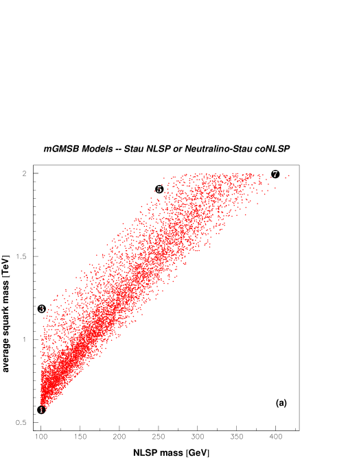
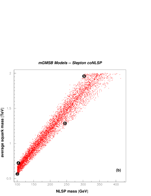
Figure 1: Scatter plots in the ($m_{\rm NLSP}$, $m_{\tilde{q}}$) plane for all relevant GMSB models generated. a) stau NLSP or neutralino-stau NLSP scenarios; b) slepton co-NLSP scenario. The eight sample models of Tabs. 1 and 2 are highlighted with their reference number.

4 Slepton Detection

The experimental signatures of heavy long-lived charged particles have been discussed both in the framework of GMSB and in more general scenarios [15, 16, 17]. The two main observables which can be used to separate these particles from muons are the high specific ionisation and the time of flight in the detector.

We concentrate here on the measurement of the time of flight which is made possible by the timing precision ($\mathrel{\;{\hbox{\raise 1.50696pt\hbox{$<$}}\kern-3.8889pt\kern-3.8889pt\hbox{\lower 2.79857pt\hbox{$\sim$}}}\;}1$ ns) and by the size of the ATLAS muon spectrometer. In the barrel part of the detector ($|\eta|<1$) the precision muon system consists of three multilayers of precision drift tubes immersed in a toroidal air-core magnetic field. The three measuring stations are located at distances of approximately 5, 7.5 and 10 meters from the interaction point. A particle crossing a drift chamber ionises the chamber gas along its path, and the electrons produced by the ionisation drift to the anode wire under the influence of an electric field. The particle position is calculated from the measurement of the drift time of the ionisation electrons to the anode wire. In order to perform this calculation a starting time $t_{0}$ for counting the drift time is needed, corresponding to the time of flight of the particle from the production point to the measuring station. For a particle travelling approximately at the speed of light, as a muon, the $t_{0}$’s for the measuring stations are parameters of the detector geometry and of the response of the front-end electronics [19]. For a heavy particle the $t_{0}$ is a free parameter, function of the $\beta$ (= v/c) of the particle. It was demonstrated with a full simulation of the ATLAS muon detector [20] that the $\beta$ of a particle can be measured by adjusting the $t_{0}$ for each station in such a way so as to minimise the $\chi^{2}$ of the reconstructed muon track. The resolution on $\beta$ obtained in [20] can be approximately parametrised as: $\sigma(\beta)/\beta^{2}=0.028$, and the resolution on the transverse momentum measurement is comparable to the one expected for muons. We have therefore simulated the detector response to NLSP sleptons by smearing the slepton momentum and $\beta$ according to the parametrisations in [20]. The full simulation has only been performed for particles produced centrally in the detector ($|\eta|\sim 0$). We conservatively use the parametrisation used in those conditions for the full $|\eta|$ coverage of the detector. In fact, for all other pseudorapidities the flight path from the interaction point to the first station, and the distance among measuring stations is larger than for $\eta=0$, and therefore the resolution on $\beta$ is expected to improve.

5 Triggering on GMSB Events

In order to evaluate the available statistics for slepton mass and lifetime measurements, we need to evaluate the trigger efficiency for the SUSY events.

The trigger system of the ATLAS experiment is described in detail in [11]. Three levels of trigger are envisaged. The first level is exclusively hardware, and the information from the muon detectors and from the calorimeters are treated separately. The second level refines the first level by connecting the information from different detectors. Finally the third level, also called ’event filter’, applies the full off line reconstruction algorithm to the data.

The quasi-stable NLSP events can be selected in the ATLAS detector by using either the muon or the calorimetric trigger.

The first option has been studied in a preliminary way in Ref. [15]. An approximate evaluation for particles with pseudorapidity $|\eta|<1$ gives an efficiency of 50% for $\beta=0.5$, increasing to basically full efficiency for $\beta=0.7$ for the trigger coincidence based on high $P_{T}$ muons ($P_{T}>20$ GeV). No comparable study exists for particles with $|\eta|>1$. In this case, due to the larger distance of the trigger station, the $\beta$ threshold for the trigger to be sensitive to the heavy sleptons will be higher than in the case of the particles produced centrally in the detector. In summary, while it is sure that part of the heavy sleptons will be accepted by the ATLAS muon trigger, at the present level of studies it is difficult to quote an efficiency for such a trigger, especially in the region of low $\beta$, which is the one yielding the best resolution for the slepton mass measurement.

In minimal GMSB models with slepton masses larger than 100 GeV, the squark masses are larger than 500 GeV. Therefore the events with production of strongly interacting sparticles will in general contain multiple high $P_{T}$ jets. As already observed in [21], if the NLSP are visible, the $P_{T}^{\rm miss}$ is generated by the neutrinos in the cascade decays, and its spectrum is relatively soft. If the $P_{T}^{\rm miss}$ is calculated only from the energy deposit in the calorimeter, neglecting the NLSP’s and the muons, the spectrum is much harder, and we recover the classical SUSY signature of $P_{T}^{\rm miss}+$jets. The first level $P_{T}^{\rm miss}$  trigger is based on the requirement of a jet with $P_{T}>50$ GeV and $P_{T}^{\rm miss}>50$ GeV (both raised to 100 GeV for the high luminosity running), where the $P_{T}^{\rm miss}$ is calculated exclusively from the energy deposit in all the calorimeter cells, and will therefore have a high efficiency for the models we are studying. Neglecting the detector smearing of the trigger thresholds, the efficiency of the $P_{T}^{\rm miss}$ trigger for the 8 example points is of order 90%. A drawback of this purely calorimetric approach is the fact that processes with low hadronic activity, such as direct slepton production and direct gaugino production are not selected. This appears clearly from the behaviour of the efficiency which is lower in the case of heavier squarks, when the fraction of events with direct gaugino production is higher. A part of these events will however be selected by the muon trigger.

It has been estimated [11] that the second level trigger will give an acceptable rate even if the transverse momenta of triggering muons is not added to the missing transverse momentum calculation. Finally the full reconstruction at the event filter level will be able to select the SUSY events by applying to the muon detector the slepton reconstruction algorithm described above. The most likely scenario is that the SUSY events will be triggered by a combined use of the muon and the calorimetric triggers, yielding an efficiency which is higher than the bare calorimeter efficiency. In the following, we will conservatively calculate the statistical errors on the measurements using the efficiencies of the calorimetric trigger.

6 Event Selection

The SM backgrounds for the considered models are processes with muons in the final state, such as the production of $\bar{t}t$, $\bar{b}b$, $W$+jets, $Z$+jets, where a muon is misidentified as a slepton.
In order to extract a clean GMSB signal from the SM background both tight identification criteria on a slepton candidate and kinematical cuts on the event structure are needed.

Figure 2: Distribution of $\beta$ for the NLSP sleptons at Points 1 and 8.

In order to select the heavy slepton, the key requirement is the presence of a track in the muon detector with a measured $\beta$ ($\beta_{meas}$) different from one. Since the resolution on the $\beta$ measurement is $\sim$0.03, by requiring $\beta_{meas}<0.91$ a rejection factor of $\sim$1000 is obtained on background muons which have $\beta=1$. The $\beta$ distribution for sleptons is shown in Fig. 2 for model points 1 and 8. In all considered cases a significant fraction of the events passes the $\beta_{meas}<0.91$ cut. Additional background rejection is obtained by comparing the momentum and the $\beta$ of the track. A track in the muon system is accepted as a slepton candidate if it satisfies the following requirements:

• $|\eta|<$2.4, to ensure that the particle is in the acceptance of the muon trigger chamber, and therefore both transverse and longitudinal component of the momentum can be measured;

• $P_{T}>10$ GeV after taking into account the energy loss in the calorimeters, to ensure that the particle traverse all the muon stations.

• It is isolated, where the isolation consists in requiring a total energy $<10$ GeV in the inner detector and in the calorimeter not associated with the candidate track in a pseudorapidity-azimuth cone $\Delta R\equiv\Delta\eta\times\Delta\phi=0.2$ around the track direction.

• $\beta_{\rm meas}<0.91$, where $\beta_{\rm meas}$ is the $\beta$ of the particle measured with the time-of-flight in the precision chambers;

• The momentum $P_{\rm meas}$ and $\beta_{\rm meas}$ should be compatible with the slepton mass $m_{\tilde{\ell}}$, corresponding to the cuts:

  $$\frac{\beta_{\rm meas}-0.05}{\sqrt{1-(\beta_{\rm meas}-0.05)^{2}}}<\frac{P_{\rm meas}}{m_{\tilde{\ell}}}<\frac{0.91+0.05}{\sqrt{1-(0.91+0.05)^{2}}}$$

Figure 3: Distribution of $P_{\rm meas}$ versus measured $\beta_{\rm meas}$ for sleptons, for Points 1 and 8. The region to the left of the thick lines in the ($\beta_{\rm meas}$, $P_{\rm meas}$) plane defines the selected slepton candidates

The region in the ($\beta_{\rm meas}$, $P_{\rm meas}$) plane defined by the last two cuts is shown for Points 1 and 8 in Fig. 3. With these cuts, the loss in slepton candidates compared to what one gets after the cut $\beta_{\rm meas}<0.91$ only is at the few percent level, with a significant gain in muon rejection, as only muons within a restricted momentum range can be misidentified as sleptons. For the lowest values of $m_{\tilde{\ell}}$ considered, the upper limit on $P_{\rm meas}$ is essential to reject the background from $W$+jets and $Z$+jets production. In fact, given the low jet multiplicity for this processes, the events passing the kinematic selection described below typically contain muons with a few hundred GeV momentum.

The isolation requirement is necessary to reduce the background from semileptonic decays of heavy quarks. A possible additional rejection on muons using the ATLAS Transition Radiation Tracker is not considered in this analysis.

The trigger requirement and the presence of a slepton candidate already yield a significant GMSB signal over the SM background from IVB + jets and top production. An overwhelming background is however expected from QCD production of $b$ jets, given the very soft kinematic requirements. The squark mass scale for the GMSB models considered ranges between 500 GeV and 2 TeV, giving a much larger transverse energy deposition in the calorimeter than the QCD background. To exploit this feature, we build an $m_{\rm eff}$ variable defined as:

$$m_{\rm eff}=\sum_{i=1}^{min(4,N_{jet})}P_{T}^{jet,i}+\sum_{i=1}^{min(2,N_{\mu})}P_{T}^{\mu,i},$$

where $\mu$ is a track reconstructed in the muon detector, including the slepton candidates. This variable is similar to the one used for SUGRA inclusive studies in [11], but also takes into account the presence of final state sleptons, and has a high efficiency also for SUSY events with no squark/gluino production.

The final requirements for GMSB event selection are therefore:

• at least one hadronic jet with $P_{T}>50$ GeV and a calorimetric $E_{T}^{\rm miss}>50$ GeV (trigger requirement);

• at least one slepton candidate as defined above;

• $m_{\rm eff}>800$ GeV;

For this indicative study, the cut on $m_{\rm eff}$ is set to a common value for all models, and the choice is aimed at reducing the SM background to a few percent of the signal for the models with lowest statistics.

In order to study the SM background, approximately 1 million events for each of the following processes: $\bar{t}t$, $W$+jets, $Z$+jets, $WW$, $WZ$, and $\sim$2 million QCD events (in different bins of $P_{T}$) were generated with the PYTHIA Monte Carlo [22]. The number of expected events after cuts for the eight GMSB models and for the main SM backgrounds for an integrated luminosity of 30 fb^-1 are given in Tab. 3.

Model	Signal	$W$+Jets	$Z$+Jets	$\bar{t}t$	QCD	Total BKGD
1	452163	9.6	6.8	5.3	8.0	29.7
2	528420	9.6	6.9	5.3	8.0	29.9
3	7437	9.5	6.9	5.3	8.0	29.9
4	147354	9.5	7.1	5.6	7.4	29.6
5	365	2.4	11.1	6.2	3.1	22.8
6	6535	2.4	11.0	6.5	3.1	23.0
7	326	1.0	5.9	3.4	0.5	10.8
8	378	1.8	8.7	4.9	2.0	17.4

Table 3: Number of events expected after cuts for the eight example models and for the major background sources. The assumed integrated luminosity is 30 fb^-1.

A number of signal events ranging from a few hundred for the models with the 2 TeV squark mass scale to a few hundred thousand for a 500 GeV mass scale survive these cuts. The corresponding background is of the order of a few tens of events, yielding a very pure sample which can be used for measuring the NLSP properties. The effect of a possible finite lifetime on the event statistics will be addressed in detail when studying the NLSP lifetime.

7 Slepton Mass Measurement

Figure 4: Distribution of the measured mass values for Points 1 and 8 as a function of $\beta$. The number of events in the scatter plot is arbitrary.

In order to perform this measurement, the particle momentum is needed. The precision chambers only provide a measurement of the momentum components transverse to the beam axis, so a measurement of the slepton pseudorapidity is needed. This can be performed either by a match with a track in the inner detector, or using the information from the muon trigger chambers. The first option requires a detailed study of the matching procedure between detectors. This study was performed for muons in [11], but the results can not be transferred automatically to the case of heavy particles for which the effect of multiple scattering in traversing the calorimetric system is much more severe.

In the case of the trigger chambers, as already discussed above, a limited time window around the beam crossing is read out, restricting the $\beta$ range for which the momentum can be measured. We therefore evaluated the statistical precision achievable for the eight example models in two different $\beta$ intervals: $0.6<\beta<0.91$ and $0.8<\beta<0.91$. For this measurement the sleptons are assumed to be stable.

From the measurements of the slepton momentum and of the particle $\beta$, the mass can be measured using the standard relation $m=p\frac{\sqrt{1-\beta^{2}}}{\beta}$. For each value of $\beta$ and momentum, the measurement error is known, and it is given by the parametrisations in Ref. [20]. Therefore, the most straightforward way to measure the mass is just to use the weighted average of all the masses calculated with the above formula. For two of the example points, we show in Fig. 4 the distribution of the measured mass as a function of $\beta$. For values of $\beta$ in the range (0.6,0.9) the spread in the mass measurement goes from $\sim 5\%$ to $\sim 15\%$, rising with $\beta$ [20]. If enough statistics at low $\beta$ is available, the measurement precision will be dominated by the events with a $\beta$ value below $\approx 0.8$.

Model	$m_{\rm NLSP}$	$N_{\rm NLSP}$	$\sigma_{m}$ (GeV)	$N_{\rm NLSP}$	$\sigma_{m}$ (GeV)
	(GeV)	$0.6<\beta<0.91$		$0.8<\beta<0.91$
1	100.1	365047	0.010	246809	0.017
2	100.4	425790	0.0093	289020	0.016
3	101.0	5933	0.084	3940	0.14
4	103.4	125220	0.018	81876	0.031
5	251.2	335	0.92	214	1.6
6	245.3	5595	0.22	3675	0.37
7	399.2	312	1.7	192	3.0
8	302.9	408	1.0	249	1.9

Table 4: Statistical errors on the NLSP mass measurement for the eight example models. The assumed integrated luminosity is 30 fb^-1.

In Tab. 4, we show the numbers of the NLSP candidates for an integrated luminosity of 30 fb^-1 and the expected errors on the mass measurement. Only the statistical errors are shown. The main systematic error on this measurement will be the uncertainty on the NLSP momentum scale, as the systematic error on the time measurement is already included in the parametrisation. We expect this uncertainty to be of order 0.1% as for the muons, if the accuracy of the energy scale measurement can be propagated to the high momentum scale considered in this analysis.

From the numbers in the table, one expects that if the NLSP is long lived, the measurement error on the NLSP mass will be dominated by the systematic error for models with a squark mass scale up to $\sim$1 TeV.

In conclusion, the slepton mass can be measured with a precision of a few permille for all the considered models with an integrated luminosity of 30 pb^-1.

8 Slepton Lifetime Measurement

The measurement of the NLSP lifetime was studied in detail in [8] for the case of a $\tilde{N}_{1}$ NLSP at a high energy $e^{+}e^{-}$ collider. In that work a number of methods were discussed in the framework of an idealised detector. By combining the different approaches a wide range in NLSP lifetimes could be covered.

The aim of this study is to perform a realistic evaluation, including the most important experimental effects, based on the detailed simulation of the response of a real detector which is already in the construction phase. For this reason we do not attempt to combine different methods, each of which would require a dedicated detector study, but we concentrate on a statistical method, which is based on the detailed study of the time of flight measurement capabilities of the ATLAS muon detector described in the previous sections.

We exploit the fact the two NLSP are produced in each event. One can therefore select events in which a slepton is detected through the time-of-flight measurement described above, and count in how many of these a second slepton candidate is found. The ratio of the number of events containing two slepton candidates to the number of events with at least one candidate is a function of the slepton lifetime. This measurement is in principle very simple, in practice it requires an excellent control of the experimental sources of inefficiency for the detection of the second slepton.

The discussion in this section is therefore organised in a series of logical steps. We first describe the principle of the method, calculating the dependence of the measured ratio on the slepton lifetime, without bothering how with real data it will be possible to connect the two quantities. From this study we estimate the achievable statistical error for the considered models, and we evaluate how a systematic uncertainty on the measured ratio propagates to the lifetime measurement. We then turn to analysing the main uncertainty sources, including the presence of background from SUSY events, the incomplete knowledge of the underlying SUSY model and the uncertainty on the detector acceptance. As a result of this analysis we estimate the range of systematic uncertainties for the experimental measurement of the lifetime. Based on this estimate in the next section we determine the achievable precision on the SUSY breaking scale $\sqrt{F}$ after the first three years of data-taking at the LHC.

8.1 The Statistical Method

We define $N_{1}$ the number of events passing the cuts discussed in Sec. 6, with the additional requirement that there be at least one candidate slepton at a distance from the interaction vertex $>10$ m. For the events thus selected we define $N_{2}$ as the number of events where a second track with a transverse momentum in excess of 10 GeV is reconstructed in the muon system. The search for the second particle should be as inclusive as possible, to minimise the corrections which should be applied to the ratio. In particular no slepton isolation is required, and the tight cuts in the ($P_{\rm meas},\beta_{\rm meas}$) plane shown in Section 6 are replaced by the requirement:

$$P_{\rm meas}>m_{\tilde{\ell}}\;\frac{\beta_{\rm meas}-0.1}{\sqrt{1-(\beta_{\rm meas}-0.1)^{2}}},$$ (6)

where $m_{\tilde{\ell}}$ is the slepton mass.

The loss in signal for this cut is less than 0.1%, thus introducing a negligible uncertainty in the measurement, and the low momentum muons in the SUSY sample are rejected. The surviving background of high momentum muons can be statistically subtracted and it will be discussed in the following section.

Figure 5: The ratio $R=N_{2}/N_{1}$ defined in the text as a function of the slepton lifetime $c\tau$. Only the curves corresponding to the model points 1, 5, 6, 8 are shown.

The ratio:

$$R=\frac{N_{2}}{N_{1}}$$

is a function of the slepton lifetime. Its dependence on the NLSP lifetime $c\tau$ in metres is shown in Fig. 5 for four of the eight model points. The curves for the model points not shown are either very similar to one of the curves we show or lie between the external curves corresponding to models 1 and 8, thus providing no additional information. Note that the curve for model 6 starts from $c\tau=2.5$ m and not from $c\tau=50$ cm, as for the other models. This is due to the large value of $M_{\rm mess}$ (cfr. Tab. 1), determining a minimum NLSP lifetime allowed by theory which is macroscopic in this case [cfr. Eqs. (3) and (5)].

The probability $P$ for a particle of mass $m$ and momentum $p$ and proper lifetime $\tau$ to travel a distance $L$ before decaying is given by the expression:

$$P(L)=e^{-mL/p{\rm c}\tau}$$

The value of $N_{2}$ is therefore a function of the momentum distribution of the slepton, which is determined by the details of the SUSY spectrum. One needs therefore to simulate the full SUSY cascade decays in order to construct the c$\tau-R$ relationship.

The statistical error in the $R$ measurement, can be evaluated as

$$\sigma(R)=\sqrt{\frac{R\;(1-R)}{N_{1}}}$$

Relevant for the precision with which the SUSY breaking scale can be measured is the error on the measured c$\tau$, which can be extracted from the curves shown in Fig. 5. This error can be evaluated as:

$$\sigma({\rm c}\tau)=\sigma(R)/\left[\frac{\partial R({\rm c}\tau)}{\partial{\rm c}\tau}\right]$$

The measurement precision calculated according to this formula is shown in Figs. 6 and 7 for the eight example points, always for an integrated luminosity of 30 fb^-1.

Figure 6: Fractional error on the measurement of the slepton lifetime $c\tau$, for model points 1 to 4. We assume an integrated luminosity of 30 fb^-1. The curves are shown for three different assumptions on the fractional systematic error on the $R$ measurement: statistical error only (full line), 1% systematic error (dashed line), 5% systematic error (dotted line).

The full line in the plots is the error on c$\tau$ if only the statistical error on $R$ is considered. The available statistics is a function of the mass scale of the strongly interacting sparticles. For mass scales between 500 and 1200 GeV, a statistical error smaller than 10% can be achieved for c$\tau$ values ranging between 1 m and several hundreds of metres. For a mass scale of 2000 GeV the statistical error is typically 10-20%. In the ideal case the details of the SUSY model are known and the $R-{\rm c}\tau$ relationship can be built from Monte Carlo, including the effect of the detector acceptance. The subtraction of the background muons from the SUSY events is the dominant contribution to the systematic error on the $N_{2}$ measurement in this ideal case, and will be treated in detail in the next section.
An additional uncertainty comes from the evaluation of the losses in $N_{2}$ because of sleptons produced outside of the $\eta$ acceptance, or absorbed in the calorimeters, or which escape the calorimeter with a transverse momentum below the cuts. This contribution is however expected to be much more important for the realistic case in which an imperfect knowledge of the SUSY model is assumed, and will be studied in that framework in a later section.
Since the uncertainty on R is a consequence of the uncertainty on the evaluation of $N_{2}$, at this level we parametrise the systematic error on R as a term proportional to R which is quadratically added to the statistical error. We choose two values, $1\%\;R$ and $5\%\;R$, and we propagate the error to the c$\tau$ measurement. The results are given as the dashed and the dotted lines in the plots in Figs. 6 and 7.

Figure 7: The same as in Fig. 6, but for model points 5 to 8.

For squark mass scales up to 1200 GeV, assuming a $1\%$ systematic error on the measured ratio, a precision better than 10% on the c$\tau$ measurement can be obtained for lifetime values between 0.5-1 m and 50-80 m. If the systematic uncertainty grows to 5%, a 10% precision can only be achieved in the range 1-10 m. If the mass scale goes up to 2 TeV, already at the level of pure statistical error a 10% precision is not achievable. One can however achieve a 20% precision over c$\tau$ ranges between 5 and 100 m, if a 1% systematic error is assumed.

8.2 Muon Background from SUSY Events

The definition of $N_{2}$, as described in the previous section, relies on a very loose identification of the second slepton candidate in order to minimise acceptance corrections, which are the dominant source of systematic uncertainties on the $N_{2}/N_{1}$ ratio.

	No cut		Cut Eq. 6
ID	1 $\mu$	$>1\mu$	1 $\mu$	$>1\mu$
1	0.37	0.14	0.027	0.00094
2	0.40	0.25	0.041	0.0011
3	0.23	0.42	0.22	0.043
4	0.39	0.39	0.16	0.014
5	0.22	0.42	0.10	0.0068
6	0.40	0.37	0.031	0.0013
7	0.36	0.34	0.026	0.
8	0.38	0.31	0.088	0.0040

Table 5: Fraction of events with one or more detected muons for the eight example points.

In the models considered for this study the charged sleptons are light, and are mostly produced in the cascade decays of charginos and neutralinos through decays of the type $\tilde{\chi}^{0}\to\tilde{\ell}\ell$ and $\tilde{\chi}^{\pm}\to\tilde{\ell}\nu$. Therefore in a significant fraction of the SUSY events muons will be produced together with the sleptons. As can be seen from the second and third column of Tab. 5, at least one muon is produced in 60-80% of the events for all considered models, and more than one muon in 30-40% of the cases for most models.

Figure 8: $\beta$ distributions for sleptons (full line histogram) and background muons (hatched histogram) for model point 4. The distributions are given for four momentum bins: a) $250<p<300$ GeV, $300<p<400$ GeV, $400<p<500$ GeV, $500<p<600$ GeV. The histogram limits exclude the peak at $\beta=1$ for the background.

Most of these muons are soft, in particular in the case of $\tilde{\tau}_{1}$ NLSP, and are rejected by the requirement in the ($P_{\rm meas},\beta_{\rm meas}$) plane which roughly corresponds to requiring the momentum of the candidate to be above twice the slepton mass. The number of muons per events after this cut are given in columns four and five of Tab. 5. The background after cuts is a function of the mass difference between the squarks and the NLSP, which determines the lepton momentum spectrum, and of the NLSP mass which determines the minimum required momentum for a candidate. The fraction ranges between a few percent and 20% of the events.

The background muons can be statistically subtracted using the observed $\beta$ distribution of the slepton candidates. For a fixed momentum $P$ of the candidate the $\beta$ of the sleptons is peaked at the value $\beta=P/\sqrt{P^{2}+m^{2}}$ where $m$ is the slepton mass, whereas the distribution for the muons is peaked at $\beta=1$ and is essentially independent of the muon momentum. As an illustration we show in Fig. 8 the $\beta$ distribution of sleptons (full line histogram) and of background muons (hatched histogram) for model point 4, which has a high background contribution. The histogram limits are set to exclude the peak at $\beta=1$ to enhance the readability. The distributions are given for four momentum bins, from 250 to 600 GeV, and the clear difference in shape between signal and background can be observed. The shape of the measured $\beta$ distribution for a given momentum only depends on the mass of the particle, and will be known for both signal and background both from detailed simulation of the detector response and from the data themselves. It will therefore be possible to measure bin by bin the relative contribution of signal and background with a likelihood fit to the observed $\beta$ distributions. The signal/background separation obtained with this technique will be further validated by comparing the momentum spectrum of the background from isolated muons with the corresponding spectrum for electrons in SUSY events.

Given the good control of the detector response expected in ATLAS and the multiple experimental handles available, the dominant contribution to the uncertainty on the measurement of $R$ from this source will be the statistical error on the background evaluation. This error will have a value of approximately $\sqrt{k/N_{1}}$, where $k$ is the number in the fourth column of Table 5. The contribution of this factor to the total error is only significant for the model points 3, 4, 5 and 8. The main effect is a 30-40$\%$ degradation of the statistical error for c$\tau$ below 10 m for Models 3 and 8. In all other cases, the effect on the c$\tau$ uncertainty from this source is smaller than the curves labelled “1%” in Figs. 6 and 7.

8.3 Model Independent Lifetime Measurement

Once the muon background has been subtracted, if the underlying SUSY model is known, $c\tau$ can simply be measured from $R$ and the curves shown in Fig. 5. Most of the SUSY mass spectrum will be measured from explicit reconstruction of exclusive decay chains, as shown in [21] and[11]. It is difficult however at this stage to evaluate the uncertainty in the construction of the $R$-c$\tau$ calibration curve from an imperfect knowledge of the SUSY model. As an alternative approach, the measurement can be performed by deconvoluting the effect of the relativistic lifetime dilatation from the measured momentum distribution of the slepton candidates. There are two cases to consider for each event, depending on whether both slepton candidates pass the cuts used to define $N_{1}$ or only one does. If only one of the two slepton candidates passes the $N_{1}$ cuts, the basic equation is:

$$N_{1}={\cal C}\sum_{i=1}^{N_{2}}W_{i},$$ (7)

with

$$W_{i}=e^{\frac{Lm}{c\tau P_{2,i}}},$$

where $L$ is the distance of the outermost muon station, $m$ is the slepton mass, $P$ its momentum, and the subscript 2 refers to the $i$-th slepton candidate which did not pass the cuts used to define $N_{1}$. The acceptance correction ${\cal C}$ is defined as the reciprocal of the detector acceptance and the experimental efficiency in detecting the second slepton candidate. Its value is strictly greater than 1.
The fraction of events in which both legs pass the criteria to define $N_{1}$ varies between $\sim$15% and 40%, increasing with the NLSP mass. In this case the expression for the event weight $W_{i}$ must be symmetrised to:

$$W_{i}=\frac{e^{-\frac{Lm}{c\tau P_{1,i}}}+e^{-\frac{Lm}{c\tau P_{2,i}}}}{e^{-\frac{Lm}{c\tau}\left(\frac{1}{P_{1,i}}+\frac{1}{P_{2,i}}\right)}}-1$$

By solving Eq. 7, the value of c$\tau$ can be measured with no reference to the underlying model. In order to evaluate the accuracy of the method, we measure c$\tau$ from the momentum distribution of the candidate sleptons for different input c$\tau$ values, assuming no statistical error and no systematic uncertainty from muon background subtraction, or from the evaluation of the acceptance correction ${\cal C}$. The fractional error on the measured c$\tau$ is shown in Fig. 9 as a function of c$\tau$ for all the 8 model points, under the above assumptions. For all the points and for the range 5–1000 m the deviation of the calculated c$\tau$ from the real value is less than 1%. The source of this small systematic deviation is the momentum smearing of the sleptons, which causes a few sleptons to be lost because they fall below the analysis cuts, and the fact that only an average correction is applied to compensate for ionisation energy loss in the calorimeters.

Figure 9: Fractional deviation of the c$\tau$ value measured using the momentum distribution of the candidates from the true value as a function of c$\tau$. The different curves shown are for the 8 example points considered. The statistical error and the systematic uncertainty on $N_{2}$ are not included in the calculation.

The experimental sources of uncertainty in Equation 7, except the $p$-scale, can be parametrised as a deviation of ${\cal C}$ from the true value. The propagation of the uncertainty on ${\cal C}$ to the c$\tau$ measurement was explicitly studied by calculating c$\tau$ with our simulated samples for all the accessible c$\tau$ range using a value of ${\cal C}$ shifted by 1$\%$ with respect to the true value. The resulting displacement in the calculated c$\tau$ value is accurately described by the curves labelled ”1%” in Figures 6 and 7.

At this point, to complete the evaluation of the systematic uncertainty on c$\tau$, we need to discuss how the acceptance correction ${\cal C}$ can be estimated in the ATLAS detector, and the expected uncertainty on its value.

8.4 Systematic Uncertainties on acceptance

The main experimental effects causing the loss of a slepton produced in a GMSB event are:

• the low energy sleptons which due to the ionisation energy loss in the calorimeters fall below the energy and transverse momentum requirements of the analysis;

• the $|\eta|$ acceptance of the detector.

An additional $\sim$5% loss, coming from the reconstruction efficiency will be measured with high precision exploiting the redundancy of the various ATLAS subdetectors, and will not be further considered.

The loss of low momentum sleptons can be estimated by studying the spectrum of the sleptons which range out in the hadronic calorimeter. These particles should present the characteristic signature of a stiff isolated highly ionising track in the inner detector depositing a small amount of energy in the electromagnetic calorimeter and all of its kinetic energy in a single tower of the hadronic calorimeter. A detailed study with full simulation of the ATLAS detector is needed to assess how well the acceptance loss can be evaluated with this technique.

For the study of the $|\eta|$ acceptance no such clear handle exists, but it should be possible to extract some indications from the observed $\eta$ distribution, and by studying the tracks up to a pseudorapidity $|\eta|<$2.7 which is the limit of the acceptance of the precision muon chambers.

The acceptance correction can also be evaluated through a Monte Carlo simulation of all the SUSY processes. The SUSY events are dominated by the production of squarks and gluinos, and the $\eta$ distribution of the sparticles produced in the hard scattering is a function of their mass. In the considered models the significant mass difference between squarks and gluinos and their decay products produces rather collimated decays, and the $\eta$ distribution of the NLSP’s is mostly determined by the mass scale of squarks and gluinos. On the other side, the lower end of the NLSP momentum spectrum is dominated by the direct production of sleptons charginos and neutralinos.

Figure 10: Acceptance correction factor calculated for 50 different GMSB models. The effects of the loss of low momentum sleptons and of the $\eta$ acceptance are included. The acceptance is given as a function of the squark mass.

In order to evaluate the spread in the value of the acceptance for different model assumptions, we have analysed 50 models with NLSP masses of 100, 200, 300, or 400 GeV, and a spread as large as possible in squark mass scale. We show in Fig. 10 the acceptance correction ${\cal C}$ for the 50 models as a function of the squark mass scale, calculated as the average of the masses of all the six squark flavours, both left and right handed. The correction varies between 4% and 1% with increasing squark mass levelling at 1% for squark masses higher than 1500 GeV. The spread in the correction factor for a fixed squark mass is below 1%. For a general SUSY model, the squark mass will be known, from the inclusive study of the $E_{T}$ distribution in SUSY events to 5-10% [11]. The situation is even better in the GMSB scenario addressed in this study, for which it will be possible to perform the full reconstruction of the decay chains of squarks [21], yielding an error on squark masses at the percent level. From these considerations, even if we conservatively assume only the constraints from inclusive studies, it should be possible to keep the uncertainty on the acceptance correction ${\cal C}$ well below the 1% mark.

9 Determining the SUSY Breaking Scale $\sqrt{F}$

Using the measured values of $c\tau$ and the NLSP mass, the SUSY breaking scale $\sqrt{F}$ can be calculated from Eq. (3), where ${\cal B}=1$ for the case where the NLSP is a slepton. From simple error propagation, the fractional uncertainty on the $\sqrt{F}$ measurement can be obtained from the experimental uncertainties on $c\tau$ on the slepton mass.

Figure 11: Fractional error on the measurement of the SUSY breaking scale $\sqrt{F}$ for model points 1 to 4. We assume an integrated luminosity of 30 fb^-1. The curves are shown for the three different assumptions on the fractional systematic error used in Figs. 6 and 7.

In Figs. 11 and 12, we show the fractional error on the $\sqrt{F}$ measurement as a function of $\sqrt{F}$ for our three different assumptions on the $c\tau$ error. The uncertainty is dominated by $c\tau$ for the higher part of the $\sqrt{F}$ range and grows quickly when approaching the lower limit on $\sqrt{F}$. This is because very few sleptons survive and the statistical error on both $m_{\tilde{\ell}}$ and $c\tau$ gets very large. If we assume a 1% systematic error on the ratio $R$ from which $c\tau$ is measured (dashed lines in Figs. 11 and 12), the error on $\sqrt{F}$ is better than 10% for $1000\;{\hbox{\raise 1.50696pt\hbox{$<$}}\kern-3.8889pt\kern-3.8889pt\hbox{\lower 2.79857pt\hbox{$\sim$}}}\;\sqrt{F}\;{\hbox{\raise 1.50696pt\hbox{$<$}}\kern-3.8889pt\kern-3.8889pt\hbox{\lower 2.79857pt\hbox{$\sim$}}}\;4000$ TeV for model points 1–4 with higher statistics. For points 5–8, in general one can explore a range of higher $\sqrt{F}$ values with a small relative error, essentially due to the large NLSP mass in these models. Note also that the theoretical lower limit (5) on $\sqrt{F}$ is equal to about 1200, 1500, 3900, 8900 TeV respectively in model points 2, 5, 6, 7, while it stays well below 1000 TeV for the other models.

Figure 12: The same as in Fig. 11, but for model points 5 to 8.

10 Conclusions

We have discussed a simple method to measure at the LHC with the ATLAS detector the fundamental SUSY breaking scale $\sqrt{F}$ in the GMSB scenarios where a slepton is the NLSP and decays to the gravitino with a lifetime in the range 0.5 m $\;{\hbox{\raise 1.50696pt\hbox{$<$}}\kern-3.8889pt\kern-3.8889pt\hbox{\lower 2.79857pt\hbox{$\sim$}}}\;c\tau_{\rm NLSP}\;{\hbox{\raise 1.50696pt\hbox{$<$}}\kern-3.8889pt\kern-3.8889pt\hbox{\lower 2.79857pt\hbox{$\sim$}}}\;1$ km. This method requires the measurement of the time of flight of long lived sleptons and is based on counting events with one or two identified NLSP’s. The achievable measurement precision critically depends on the uncertainties in evaluating the experimental inefficiencies in the NLSP detection. We have performed a particle level simulations for eight representative GMSB models, some of them being particularly hard due to low statistics. The experimental study is based on a parametrisation of the ATLAS muon detector response to sleptons, based on a detailed full simulation study. The careful consideration of the possible sources of uncertainty allows us to conclude that the systematic uncertainty affecting the measurement will be at the percent level. In this framework, a level of precision of a few 10’s % on the SUSY breaking scale measurement can be achieved in significant parts of the $1000\;{\hbox{\raise 1.50696pt\hbox{$<$}}\kern-3.8889pt\kern-3.8889pt\hbox{\lower 2.79857pt\hbox{$\sim$}}}\;\sqrt{F}\;{\hbox{\raise 1.50696pt\hbox{$<$}}\kern-3.8889pt\kern-3.8889pt\hbox{\lower 2.79857pt\hbox{$\sim$}}}\;30000$ TeV range, for all models considered. The range of the measurement could be extended through the direct detection of NLSP decays either inside the inner detector cavity or inside the muon spectrometer. A detailed detector simulation for these signatures would be needed in order to assess the possible gain in sensitivity.

We stress that the results of the present analysis cover larger classes of theoretical frameworks. In particular, any model implying the presence of long-lived particles decaying into leptonic final states through the production of primary heavy particles with mass of order 1 TeV (parameter that guarantees a crucial suppression of the SM background) can be analysed according to similar strategies.

Acknowledgements

We would like to acknowledge useful discussions with many members of the ATLAS Collaboration about the details of the ATLAS experimental setup. Special thanks go to Frank Paige for discussions on the signatures of the slow sleptons and for useful comments on the paper, and to Fabiola Gianotti for carefully reading the manuscript and for punctual remarks on the experimental assumptions underlying our analysis. S. A. and G. P. thank the organisers of the Workshop “Physics at TeV Colliders”, for the hospitality and the pleasant and productive atmosphere in Les Houches where this work was started.

References

- [1] For a recent pedagogical review of supersymmetry and supersymmetry breaking, see S. P. Martin, “A Supersymmetry Primer”, in “Perspectives on Supersymmetry”, G. L. Kane ed., World Scientific 1998, hep-ph/9709356 and references therein.
- [2] M. Dine, W. Fischler, M. Srednicki, Nucl. Phys. B189 (1981) 575; S. Dimopoulos, S. Raby, Nucl. Phys. B192 (1981) 353; M. Dine, W. Fischler, Phys. Lett. 110B (1982) 227; M. Dine, M. Srednicki, Nucl. Phys. B202 (1982) 238; M. Dine, W. Fischler, Nucl. Phys. B204 (1982) 346; L. Alvarez-Gaumé, M. Claudson, M. B. Wise, Nucl. Phys. B207 (1982) 96; C. R. Nappi, B. A. Ovrut, Phys. Lett. 113B (1982) 175; S. Dimopoulos, S. Raby, Nucl. Phys. B219 (1983) 479.
- [3] M. Dine, A. E. Nelson, Phys. Rev. D 48 (1993) 1277; M. Dine, A. E. Nelson, Y. Shirman, Phys. Rev. D 51 (1995) 1362; M. Dine, A. E. Nelson, Y. Nir, Y. Shirman, Phys. Rev. D 53 (1996) 2658.
- [4] For a review, see G. F. Giudice, R. Rattazzi, Phys. Rep. 322 (1999) 419.
- [5] S. Dimopoulos, S. Thomas, J. D. Wells, Phys. Rev. D 54 (1996) 3283; Nucl. Phys. B488 (1997) 39.
- [6] J. A. Bagger, K. Matchev, D. M. Pierce, R. Zhang, Phys. Rev. D 55 (1997) 3188.
- [7] S. Ambrosanio, G. D. Kribs, S. P. Martin, Phys. Rev. D 56 (1997) 1761.
- [8] S. Ambrosanio, G. A. Blair, Eur. Phys. J. C 12 (2000) 287–321.
- [9] P. Fayet, Phys. Lett. 70B (1977) 461; Phys. Lett. 86B (1979) 272; Phys. Lett. B 175 (1986) 471 and in “Unification of the fundamental particle interactions”, eds. S. Ferrara, J. Ellis, P. van Nieuwenhuizen (Plenum, New York, 1980) p. 587.
- [10] A relevant example is discussed in: S. Ambrosanio, G. D. Kribs, S. P. Martin, Nucl. Phys. B516 (1998) 55.
- [11] The ATLAS Collaboration, “ATLAS Detector and Physics Performance Technical Design Report”, ATLAS TDR 15, CERN/LHCC/99-15 (1999).
- [12] An updated, generalised and Fortran-linked version of the program used in Ref. [7]. It generates minimal and non-minimal GMSB and SUGRA models. For inquiries about this software package, please send e-mail to ambros@mail.cern.ch.
- [13] H. Baer, F. E. Paige, S. D. Protopopescu, X. Tata, hep-ph/9305342; hep-ph/9804321.
- [14] E. Richter-Was, D. Froidevaux, L. Poggioli, “ATLFAST 2.0: A Fast Simulation Package for ATLAS”, ATLAS Internal Note ATL-PHYS-98-131 (1998).
- [15] A. Nisati, S. Petrarca, G. Salvini, Mod. Phys. Lett. A12 (1997) 2213.
- [16] M. Drees, X. Tata, Phys. Lett. B 252 (1990) 695.
- [17] J. L. Feng, T. Moroi, Phys. Rev. D 58 (1998) 035001.
- [18] S. P. Martin, J. D. Wells, Phys. Rev. D 59 (1999) 035008.
- [19] A. Nisati, “Preliminary Timing Studies of the Barrel Muon Trigger System”, ATLAS Internal Note ATL-DAQ-98-083 (1998).
- [20] G. Polesello, A. Rimoldi, “Reconstruction of Quasi-stable Charged Sleptons in the ATLAS Muon Spectrometer”, ATLAS Internal Note ATL-MUON-99-06.
- [21] I. Hinchliffe, F. E. Paige, Phys. Rev. D 60 (1999) 095002.
- [22] T. Sjöstrand, Comp. Phys. Comm. 82 (1994) 74.