Abstract

We identify and resum corrections associated with the kinematic recoil of the hard scattering against soft-gluon emission in single-particle inclusive cross sections. The method avoids double counting and conserves the flow of partonic energy. It reproduces threshold resummation for high-$p_{T}$ single-particle cross sections, when recoil is neglected, and $Q_{T}$-resummation at low $Q_{T}$, when higher-order threshold logarithms are suppressed. We exhibit explicit resummed cross sections, accurate to next-to-leading logarithm, for electroweak annihilation and prompt photon inclusive cross sections.

1. Introduction

A large class of hard-scattering cross sections in QCD are factorized into convolutions of parton distributions and fragmentation functions with hard-scattering functions [1]. Important and representative examples are Higgs production and Drell-Yan cross sections, at measured invariant mass $Q$ and transverse momentum $Q_{T}$. We shall refer to these reactions collectively as electroweak annihilation. At fixed, large $Q_{T}$, electroweak annihilation cross sections are written in collinear-factorized form as

$${d\sigma_{AB\to V}\over dQ^{2}dQ_{T}^{2}}=\sum_{ab}\int dx_{a}\;\phi_{a/A}(x_{a},\mu)\,\int dx_{b}\;\phi_{b/B}(x_{b},\mu)\;\hat{\sigma}_{ab\to V}\left(Q^{2}/\hat{s},Q_{T}^{2}/Q^{2},Q^{2}/\mu^{2},\mu,\alpha_{s}(\mu)\right)\,,$$ (1)

in terms of evolved, nonperturbative distributions (densities) $\phi_{a/A}(x,\mu)$ of parton $a$ in hadron $A$, and hard-scattering functions $\hat{\sigma}_{ab\to V}\left(Q^{2}/\hat{s},Q_{T}^{2}/Q^{2},Q^{2}/\mu^{2},\mu,\alpha_{s}(\mu)\right)$, computed as power series in $\alpha_{s}$. Here $\hat{s}\equiv x_{a}x_{b}S$ is the partonic invariant mass squared, while $\mu$ is a factorization scale, which for the time being we equate to the renormalization scale. General single-particle inclusive (1PI) cross sections for photons and light hadrons at high $p_{T}$ take a similar form, including a fragmentation function.

Many hard-scattering functions have been computed to next-to-leading order (NLO) in $\alpha_{s}(\mu)$. Analytic calculations of still higher-order contributions [2] to $\hat{\sigma}$ are as yet too complex to carry out, except for fully inclusive processes, such as the Drell-Yan production of lepton pairs at measured invariant mass [3]. Nevertheless, general arguments show that the functions $\hat{\sigma}$ are infrared safe to all orders [4].

Starting at NLO, the computation of $\hat{\sigma}$ involves cancellations between soft gluon emission and virtual corrections. These cancellations produce plus distributions and delta functions, which require integration against smooth functions, such as parton densities. The finite integrals, in turn, are potential sources of numerically large corrections at each order in perturbation theory. Because of their connection to soft-gluon emission, however, such corrections can sometimes be resummed to all orders in perturbation theory.

For example, in Eq. (1), $\hat{\sigma}_{ab\to V}$ includes distributions that are singular at partonic threshold, $\hat{s}=Q^{2}$, where partons $a$ and $b$ have just enough invariant mass to produce the observed final state. Defining $z=Q^{2}/\hat{s}$, we find at $n$th order singularities as strong as $\alpha_{s}^{n}[(1-z)^{-1}\ln^{2n-1}(1-z)]_{+}$. Threshold resummations, which organize these distributions, have been developed for a large class of cross sections [5, 6, 7]. Although these singularities are manifest in $\hat{\sigma}_{ab\to V}$, they do not generally result in large logarithms in the physical cross section, because they are smoothed by the integrals over $x_{a}$ and $x_{b}$ in Eq. (1). Thus, threshold resummation is not a summation of kinematic logarithms in the physical cross section. It is rather an attempt to quantify the effect on the physical cross section of a well-defined set of corrections in $\hat{\sigma}$ to all orders.

Threshold singularities are not the only singular distributions encountered in the computation of $\hat{\sigma}$. In addition, the perturbative cross section is singular up to $\alpha_{s}^{n}[(1/Q_{T}^{2})\,\ln^{2n-1}(Q_{T}^{2}/Q^{2})]_{+}$ in $\hat{\sigma}$, Eq. (1), when the transverse momentum, $Q_{T}$, of the electroweak boson is small compared to its mass, $Q$ [8, 9]. At each order, $Q_{T}$ is balanced by soft gluons, and singularities in the differential cross section at $Q_{T}=0$ reflect collinear divergences in $\hat{\sigma}$ not eliminated by factorization. These divergences, resummed or not, cancel in the $Q_{T}$-integrated cross section, even before the integrals over the partonic fractions $x_{a}$ and $x_{b}$, although the remainder is still singular at partonic threshold.

Much of the recent interest in soft-gluon recoil effects has centered on the normalization and $p_{T}$-dependence of single-particle inclusive cross sections [10], particularly direct-photon production at fixed-target energies [11, 12, 13, 14, 15, 16, 17]. The formalism of $Q_{T}$ resummation for Eq. (1) is not immediately applicable to inclusive high-$p_{T}$ cross sections, because in this case most of the transverse momentum of the observed particle is recoil against other high-$p_{T}$ particles, while only a small portion is from soft radiation. A rough-and-ready approach to soft-gluon radiation is to introduce intrinsic transverse momentum for the partons in factorized expressions like Eq. (1), typically in the form of an energy-dependent Gaussian smearing of standard parton densities, which enhances the cross section. This method, however, certainly involves double counting, and does not respect the conservation of partonic energy. Some time ago, Li and Lai explored the possibility that nonperturbative $k_{T}$ smearing in high-$p_{T}$ cross sections has the same origin as in the low-$Q_{T}$ Drell-Yan cross sections described by the $Q_{T}$-resummation formalism [17]. More recently, Li [18] has shown how threshold and transverse momentum resummation may be derived from the same parton distribution, defined in transverse momentum space, as in Ref. [9].

When the conservation of energy is taken into account, however, it is no longer obvious whether the inclusion of recoil effects will lead to an enhancement or a suppression, because the extra radiation involves a number of competing effects. On the one hand, a substantial $k_{T}$ from initial-state radiation allows a softer $2\to 2$ subprocess at the hard scattering, which clearly acts toward enhancement. On the other hand, the extra energy of the initial-state radiation drives the physical parton distributions to larger $x$, which may more than make up for enhancements in the hard scattering if the distributions are decreasing with $x$. At the same time, larger $x$ is associated with larger threshold enhancements in general. The only way to estimate the influence of recoil effects on cross sections is to develop a self-consistent resummation formalism.

In this paper, we shall take up, and we hope clarify, this general viewpoint. Our reasoning is based on a generalization of threshold resummation which, as we have seen, controls singular distributions at $z=1$. For electroweak annihilation and single-particle inclusive cross sections, such contributions are always associated with an underlying $2\to 2$ hard scattering [5]. We use the $2\to 2$ subprocess to define the relevant transverse momentum $Q_{T}$, whose singularities we resum. The recoil we discuss below is always the recoil of a $2\to 2$ subprocess. Thus, just as for threshold resummation, we reorganize a well-defined set of higher order corrections in hard scattering functions, always working at leading power in the hard scale, $Q$, within collinear factorization. We do not exclude the possibility of nonperturbative effects, however. Indeed, we will observe that nonperturbative corrections arise quite naturally from our resummed expressions. A summary of our results, applied to prompt photon cross sections, was described in Ref. [19].

Let us offer a few additional comments on nonperturbative effects in these cross sections. Nonperturbative effects play a crucial role in the phenomenological description of electroweak annihilation cross sections at low $Q_{T}$, even for a large final state mass scale $Q$. This is the case, even after the resummation of logarithms of $Q_{T}/Q$ that can give a well-defined perturbative prediction for small $Q_{T}$. Incorporating nonperturbative effects, of course, requires the introduction of new parameters [8, 20, 21]. In each of these cases, the form of nonperturbative corrections is suggested by perturbation theory [22, 23, 24]. In contrast, nonperturbative effects (beyond fragmentation functions) have not been incorporated in prompt photon and other single-particle inclusive cross sections, where there is no need for them at fixed order in perturbation theory. For threshold-resummed cross sections the situation is somewhat more subtle, but “minimal” formulations of threshold resummation allow for a class of purely perturbative predictions [25, 26], with no new parameters. Of course, the existence of such a formalism does not by itself preclude the importance of nonperturbative effects. In this paper, we develop a perturbative formalism that links both sorts of cross sections, and which is consistent with known results that have suggested nonperturbative corrections at measured $Q_{T}$ in electroweak annihilation. Part of our goal is to open the door, not only to further perturbative analysis, but also to the study of similarities and differences in the roles of nonperturbative corrections in these cases.

We choose to work in the formalism of collinear factorization because we do not wish to introduce a new set of phenomenological parton distributions, depending on transverse as well as longitudinal degrees of freedom, except where absolutely necessary . The resulting combination of threshold and transverse momentum resummations is at least as technically challenging as NLO factorization, let alone $Q_{T}$-resummation, and the new formalism will require some time to understand and develop as a practical tool. We therefore do not attempt to draw immediate phenomenological conclusions in this paper. Instead, we shall concentrate on the formal development, and (especially in Appendix A) the theoretical underpinning of these ideas. We have attempted to be as explicit as possible in our arguments and in specifying the functions whose momentum-dependence controls the set of higher-order corrections that we study. This has resulted in a paper of substantial, although we hope not excessive, length.

We begin in Sec. 2 with a treatment of electroweak annihilation processes, such as Drell-Yan and Higgs production, whose singular behavior at vanishing transverse momentum has been studied intensively over the years [8, 9], and which is in many ways the archetype for resummation. We show how to introduce threshold resummation consistently at measured $Q_{T}$ for these processes. Our approach to resummation is through a “refactorization” of partonic cross sections near threshold [7, 27]. In this discussion, we shall review the refactorizations at the basis of $Q_{T}$ and threshold resummations, and define a set of new functions which control singular behavior in $1-z$ and $Q_{T}$ jointly. These will serve as building blocks both for electroweak annihilation cross sections, in Sec. 3, and for single-particle inclusive processes, in Sec. 4.

Resummation at threshold and in transverse momentum is most often formulated in Mellin ($N$) moment space for the former, and impact parameter ($b$) space for the latter. Resummed logarithms of these parameters exponentiate in the relevant limits, so that the resummed cross sections are inverse transforms. In Sec. 3 we resum logarithms of $b$ and $N$ in the electroweak annihilation cross sections. We begin by deriving a relation for the hadronic $d\sigma/dQ^{2}dQ_{T}^{2}$ in terms of parton distributions, eikonal cross sections for partons, and universal anomalous dimensions. We observe that this jointly-resummed cross section determines the pattern of power corrections in $Q$ and $b$ that are implied by the behavior of the strong coupling in perturbation theory. In particular, we find that in QCD such power corrections appear only at even powers of the invariant mass $Q$ and impact parameter $b$.

Sec. 4 deals first with prompt photon production, and then with general high-$p_{T}$ single-hadron or photon inclusive cross sections. For the former, we derive the joint resummation applied in Ref. [19], and for the latter we discuss the additional resummation associated with fragmentation.

Explicit NLL expressions for jointly-resummed exponents in electroweak annihilation and prompt photon production are given in Sec. 5, along with a few comments on the source of enhancement at NLL. Following our conclusions, we include two appendices. The first gives the necessary arguments for factorization and refactorization, and the second gives explicit one-loop results for some of the functions that play an important role in the refactorizations of hard-scattering cross sections.

2. Refactorization for Electroweak Annihilation

As above, $Q$ denotes the mass of an electroweak final state, such as a vector boson, a Drell-Yan pair or a Higgs boson. The cross section $d\sigma/dQ^{2}dQ_{T}^{2}$, at measured $Q^{2}$ and $Q_{T}$, given in factorized form in Eq. (1), is singular at $Q_{T}=0$, order-by-order in perturbation theory. There are a number of phenomenological applications of $Q_{T}$-resummation for these singularities [20, 21]. We know of no simultaneous application of threshold resummation, however, although the cross sections are singular as well at partonic threshold, $\hat{s}=Q$.

As pointed out above, distributions that are singular at threshold are smoothed in the physical cross section by integration with the parton densities. Nevertheless, there is a good deal to be learned by resumming singular behavior from the limit $\hat{s}\to Q^{2}$, even at fixed, measured $Q_{T}$ [28]. To derive a cross section resummed both in threshold and $Q_{T}$ variables, we study partonic cross sections $a+b\to V+X$ near threshold, where $a$ and $b$ are partons, and where $V$ denotes the heavy electroweak final state $V={\rm W,Z,H}$, etc. We begin by formulating the problem in a standard form, through collinear factorization.

In this section, which is rather technical in parts, we lay the groundwork for our derivation of jointly resummed cross sections. We have chosen to present our new formalism in the context of a review of existing resummations, for the purpose of motivation, and also to bring together a set of results and methods that are somewhat scattered in the literature. It may be helpful, therefore, to outline the contents and aims of the subsections that follow.

We begin (subsection 2.1) by relating the hard-scattering functions that we will resum to partonic cross sections. In subsection 2.2, we review existing refactorizations for partonic cross sections, which have been used to derive resummations for electroweak annihilation at low transverse momentum [9] and at partonic threshold [5, 6]. We then go on to present a novel refactorization that combines the two (Eq. (9)), and observe how refactorization provides a natural formulation of the effects of recoil. The all-orders justifications for all of these refactorizations are presented in Appendix A. Eq. (9) involves new perturbative functions, denoted ${\cal R}_{i/j}$. The field-theoretic content of these functions is the subject of subsection 2.3, which begins with a review of the analogous definitions for light cone parton distributions [29], as well as the fixed-energy distributions introduced in Ref. [5]. Each of the refactorization theorems in subsection 2.2 also includes a function that describes coherent radiation, which summarizes the interference between emission by incoming and outgoing hard partons. An analysis of coherent radiation is especially important for processes in which colored particles emerge from the hard scattering [7], the simplest of which is prompt photon production. This interference may be treated in eikonal approximation. The analysis of the eikonal approximation to soft gluon radiation is the subject of subsection 2.4, in which various eikonal analogs of the densities in 2.3 are introduced. Finally (subsection 2.5), we review the use of Mellin and Fourier transforms to isolate hard-scattering functions. The new results derived in this section are applied in Sec. 3 to electroweak annihilation, and in Sec. 4 to single-particle inclusive cross sections.

2.1. The hard-scattering function

Although the hard-scattering function $\hat{\sigma}_{ab\to V}$ in Eq. (1) is singular at $Q_{T}=0$, these singularities may be determined at the same time as threshold singularities at $Q^{2}/\hat{s}=1$. To be specific, we shall derive an expression for $\hat{\sigma}_{ab\to V}$ in terms of its moments with respect to $z\equiv Q^{2}/\hat{s}$,

$$\hat{\sigma}_{ab\to V}\left(N,Q_{T}^{2}/Q^{2},Q^{2}/\mu^{2},\mu,\alpha_{s}(\mu)\right)=\int_{0}^{1}dz\;z^{N-1}\;\hat{\sigma}_{ab\to V}\left(z,Q_{T}^{2}/Q^{2},Q^{2}/\mu^{2},\mu,\alpha_{s}(\mu)\right)\,,$$ (2)

where for economy of notation, we denote the transform of $\hat{\sigma}_{ab\to V}$ with respect to $z$ ($Q_{T}$) by its argument $N$ ($b$). The hat refers to its role as a hard-scattering function, from which collinear divergences are subtracted. The inverse of the Mellin moment (2) is, as usual,

$$\hat{\sigma}_{ab\to V}\left(z,Q_{T}^{2}/Q^{2},Q^{2}/\mu^{2},\mu,\alpha_{s}(\mu)\right)=\int_{C-i\infty}^{C+i\infty}{dN\over 2\pi i}\;z^{-N}\;\hat{\sigma}_{ab\to V}\left(N,Q_{T}^{2}/Q^{2},Q^{2}/\mu^{2},\mu,\alpha_{s}(\mu)\right)\,.$$ (3)

We are able to construct $\hat{\sigma}_{ab\to V}(N)$ because it also emerges from the factorization of partonic cross sections with respect to $\tau\equiv Q^{2}/S$. Up to corrections due to parton mixing, which we may neglect to leading power in the moment variable, we have, from Eq. (1),

$$\hat{\sigma}_{ab\to V}\left(N,Q_{T}^{2}/Q^{2},Q^{2}/\mu^{2},\mu,\alpha_{s}(\mu)\right)={1\over\tilde{\phi}_{a/a}(N+1,\mu)\;\tilde{\phi}_{b/b}(N+1,\mu)}\;\int_{0}^{1}d\tau\;\tau^{N-1}{d\sigma_{ab\to V}\over dQ^{2}dQ_{T}^{2}}\,.$$ (4)

The moments, $\tilde{\phi}_{i/i}(N+1,\mu)$, of the parton-in-parton distributions cancel collinear singularities in the moments of the partonic cross section, and the right-hand side of this expression is infrared safe, order-by-order in perturbation theory when $Q_{T}\neq 0$. Our goal now is to determine the singular structure of $\hat{\sigma}_{ab\to V}$ at both $z=1$ and at $Q_{T}=0$. To control these singularities, we follow Refs. [5, 30, 31, 32, 33, 34], and refactorize the (collinear-regularized) partonic cross section $d\sigma_{ab\to V}/dQ^{2}dQ_{T}^{2}$ in this limit. The discussion of the following subsection applies entirely to these, purely partonic, cross sections.

2.2. Refactorization and recoil in the partonic cross section

To motivate the refactorization appropriate to joint resummation in $Q_{T}$ and $1-z$, it may be useful to review the relevant features of the separate resummation formalisms for transverse momentum and threshold. We will continue to work in the context of perturbation theory as in Eq. (4), because our aim is always to analyze higher orders in partonic hard-scattering functions. Each of the refactorizations given below involves the introduction of new parton distributions, variously at measured transverse momentum and/or energy fraction. The new functions are not to be interpreted as physically-accessible distributions. Rather, they are perturbative constructs useful for the analysis of the hard-scattering functions of Eq. (4).

In the formalism of Ref. [35], the measured-$Q_{T}$ cross section is written as a convolution of (parton-in-parton) distributions ${\cal P}_{i/j}(x,{\bf k})$, at fixed parton transverse momentum ${\bf k}$, and light-cone momentum fraction $x$, along with an additional, eikonal function $U_{cd}({\bf q})$ that describes coherent soft-gluon emission at fixed transverse momentum,

$${d\sigma_{ab\to V}\over dQ^{2}d^{2}{\bf Q}_{T}} = \sum_{cd}\ \sigma_{cd\to V}^{({\rm 0)}}(Q^{2})\;h_{cd}^{\rm(kt)}(\alpha_{s}(Q))\;\int dx_{a}d^{2}{\bf k}_{a}\,{\cal P}_{c/a}(x_{a},{\bf k}_{a},Q)\int dx_{b}d^{2}{\bf k}_{b}\,{\cal P}_{d/b}(x_{b},{\bf k}_{b},Q)$$ (5)

$$\times\int d^{2}{\bf q}\ U_{cd}({\bf q}/\mu,\alpha_{s}(\mu))\ \delta(Q^{2}-x_{a}x_{b}S)\ \delta^{2}\left({\bf Q}_{T}+{\bf k}_{a}+{\bf k}_{b}+{\bf q}\right)+Y_{\rm kt}\,,$$

where $\sigma^{(0)}$ is the Born total cross section for the process, for example, $\sigma_{a\bar{a}\to\gamma^{*}}^{(0)}=4\pi\alpha^{2}/3N_{C}\,Q^{2}$, with $N_{C}$ the number of colors. The remainder, $Y_{\rm kt}$, does not diverge as a power at $Q_{T}=0$. Note that because the functions ${\cal P}_{i/j}$ are defined at measured ${\bf k}$, no factorization scale is necessary, although the distributions still depend on the overall momentum scale $Q$. The variable $\mu$ in the arguments of $U$ is therefore a renormalization scale. The additive convolution in this expression implies that the cross section breaks up into a product under a Fourier transform to impact parameter ($b$) space [8]. The function $h_{cd}^{\rm(kt)}(\alpha_{s}(Q))=1+{\cal O}(\alpha_{s}(Q))$ absorbs hard-gluon corrections that appear in coefficients of $\delta^{2}({\bf Q}_{T})$. The combination $\sigma^{(0)}\;h^{\rm(kt)}$ is a truly short-distance function, dominated by lines off-shell by ${\cal O}(Q^{2})$ [36]. In contrast, the full hard-scattering function in Eq. (4) in general contains lines that are off-shell only by ${\cal O}(Q_{T}^{2})$. This hierarchy of perturbative scales is characteristic of resummation. We shall use the term “short-distance” to refer specifically to functions that depend only on the largest scale, $Q$ in this case.

The refactorized cross section for threshold resummation, with integrated ${\bf Q}_{T}$, has many of the same features. Now, however, the parton-in-parton distributions $\psi_{i/j}(x)$ are defined at measured fraction of the energy of parton $j$ (in the center-of-mass frame for the hard scattering), rather than light-cone fraction, as is the new eikonal function $U_{cd}(w_{s})$, with total energy $w_{s}Q$ for soft gluon radiation into the final state. Working to leading power in $1-Q^{2}/S$ leads to important simplifications. First, the nondiagonal parton-in-parton distributions, $\psi_{c/a}(x,Q)$ begin at order $\alpha_{s}$ with the emission of a soft fermion (not a pair) into the final state, which results in a suppression of order $1-x$ in the distribution, and of $1-Q^{2}/S$ in the cross section [5]. To leading power, therefore, we may neglect parton mixing, just as at leading power in the moments, Eq. (4). The refactorized expression is [5]

$${d\sigma_{ab\to V}\over dQ^{2}} = {1\over S}\;\sigma_{ab\to V}^{({\rm 0)}}(Q^{2})\;h_{ab}^{\rm(th)}(\alpha_{s}(Q))\ \int dx_{a}\,\psi_{a/a}(x_{a},Q)\int dx_{b}\,\psi_{b/b}(x_{b},Q)$$ (6)

$$\times\int dw_{s}\ U_{ab}(w_{s}Q/\mu,\alpha_{s}(\mu))\ \delta\left(1-{Q^{2}/S}-(1-x_{a})-(1-x_{b})-w_{s}\right)+Y_{\rm th}\,,$$

where $Y_{\rm th}$ is nonleading by a power of $1-Q^{2}/S$. Even though transverse momenta in $\psi$ are integrated, the phase space for radiation is finite for fixed parton energy, and $\mu$ again denotes the renormalization scale. An explicit definition of $\psi_{c/a}$ as a matrix element will be given below. The remainder, $Y_{\rm th}$, does not diverge as a power of $1-Q^{2}/S$ at threshold. The short-distance function $h_{ab}^{\rm(kt)}=1+{\cal O}(\alpha_{s})$ organizes infrared safe coefficients of $\delta(1-z)$ in this case.

It is most natural to analyze the cross section near threshold, Eq. (6), in terms of a Laplace transform, $\int d\tau\exp[-N(1-\tau)]$, with $\tau=Q^{2}/S$. For $N$ large, we can readily relate this Laplace transform to the Mellin moments in Eq. (4). This follows because generally,

$${\rm e}^{-N(1-\xi)}\sim\xi^{N}\,,$$ (7)

with corrections that are suppressed by a power of $N$, and because in Eq. (6),

$$1-(1-x_{a})-(1-x_{b})-w_{s}\sim x_{a}x_{b}(1-w_{s})+{\cal O}\left(\left[1-Q^{2}/S\right]^{2}\right)\,.$$ (8)

The Laplace moments of Eq. (6) are therefore equivalent to its Mellin moments to leading power in $N$, and hence in $1-Q^{2}/S$.

The close correspondence between the factorizations at low $Q_{T}$ and near threshold makes it rather natural to combine the two. We therefore propose a convolution at fixed transverse momentum and energy fraction:

$${d\sigma_{ab\to V}\over dQ^{2}d^{2}{\bf Q}_{T}} = {1\over S}\;\sigma_{ab\to V}^{({\rm 0)}}(Q^{2})\;h_{ab}^{\rm(j)}(\alpha_{s}(Q))\;\int dx_{a}d^{2}{\bf k}_{a}\,{\cal R}_{a/a}(x_{a},{\bf k}_{a},Q)\;\int dx_{b}d^{2}{\bf k}_{b}\,{\cal R}_{b/b}(x_{b},{\bf k}_{b},Q)$$ (9)

$$\hskip 14.22636pt\times\int dw_{s}d^{2}{\bf k}_{s}\,U_{ab}(w_{s},Q,{\bf k}_{s})\;\delta(1-Q^{2}/S-(1-x_{a})-(1-x_{b})-w_{s})$$

$$\hskip 14.22636pt\times\;\delta^{2}\left({\bf Q}_{T}+{\bf k}_{a}+{\bf k}_{b}+{\bf k}_{s}\right)+Y_{\rm j}\,.$$

The short-distance function $h_{ab}^{\rm(j)}(\alpha_{s})$ is again an infrared-safe series in the running coupling, which begins with unity at zeroth order, and which absorbs, in this case, the coefficients of $\delta(1-z)\,\delta^{2}({\bf Q}_{T})$ at one loop and beyond. The remainder $Y_{\rm j}$ is free of power singularities at ${\bf Q}_{T}=0$ at leading power in $1-Q^{2}/S$. As in threshold resummation, only flavor-diagonal hard scatterings contribute at ${\cal O}[1/(1-Q^{2}/S)]$. It is important to note that in terms that are not singular in $Q_{T}$, this leading power emerges only after integration over $Q_{T}$. This is because at fixed energy $(1-z)Q$, the phase space in $Q_{T}$ behaves as: $\int_{0}^{Q^{2}(1-z)^{2}}dQ_{T}^{2}=(1-z)^{2}Q^{2}$.

Eq. (9), and indeed each of the refactorizations discussed above, may be represented as in Fig. 1. In the terminology of Ref. [4] and Appendix A below, Figure 1 represents the general “leading regions” in momentum space for this cross section. The subdiagrams $J_{a,b}$ include lines collinear to the incoming partons, $H$ lines off-shell by order $Q$, and $U$ soft radiation.

Figure 1: Leading region for electroweak annihilation in cut diagram form. The vertical line represents the final state that includes an electroweak boson, labelled $Q$. The subdiagrams $J_{a}$, $J_{b}$, $U_{ab}$ and $H$ incorporate, respectively, on-shell lines with momenta collinear to $p_{a}$, lines with on-shell momenta parallel to $p_{b}$, lines with soft momenta, and lines off-shell by order $Q$.

The refactorizations of Eqs. (5) and (9) themselves define the concept of recoil that we will use in this paper. The short-distance function $\sigma^{(0)}\;h^{\rm(kt)}$ is computed with on-shell external momenta, collinear to the incoming lines. All unintegrated transverse momentum dependence is contained in the generalized parton densities ${\cal P}$ in (5) and ${\cal R}$ in Eq. (9). The dependence of highly off-shell lines on the transverse momenta ${\bf k}_{a}$ and ${\bf k}_{b}$ of initial-state partons is to be absorbed into higher orders of the short-distance function, by the usual methods of collinear factorization. On the other hand, in both transverse momentum and joint resummation, we retain the kinematic linkage of the partonic transverse momentum with the electroweak final state. This is what we shall mean by including recoil effects.

2.3. Matrix elements

The refactorization theorems above, and the resummations derived from them, involve a number of new functions. We now give explicit definitions for the various parton distributions, $\cal P$, ${\cal R}$ and $\psi$, when the incoming partons are quarks, as well as for the eikonal functions $U$. Gluonic distributions can be defined similarly, following Ref. [29].

The parton densities ${\cal R}_{a/a}$ and the eikonal functions $U_{f\bar{f}}$, defined at fixed energy and transverse momentum are, like Eq. (9) itself, straightforward variations of functions identified for the $Q_{T}$ and threshold resummed cases. The prototype for these expressions is the partonic light-cone distribution, written as [29]

$$\phi_{f/f}(x,\mu,\epsilon)=\frac{1}{4N_{C}}\int{d\lambda\over 2\pi}\;{\rm e}^{-i\lambda xp^{+}}\;\langle f(p)|\bar{q}_{f}\big{(}\lambda u)\gamma\cdot u\;q_{f}(0)|f(p)\rangle\,,$$ (10)

where $\mu$ is the scale at which the product of quark fields, which are connected by a lightlike separation, $\lambda u^{\mu}$, $u^{2}=0$, is renormalized. An average over colors and spins is included in the definition. In this expression, we have suppressed an ordered exponential, $\Phi_{u}^{(q)}\left(\lambda,0;0\right)$, which we shall also refer to as a nonabelian phase line, of the gauge field along the light cone vector between the quark fields, in the notation

$$\Phi_{\beta}^{(f)}(\lambda_{2},\lambda_{1};X)=P\exp\left(-ig\int_{\lambda_{1}}^{\lambda_{2}}d{\eta}\;{\beta}{\cdot}A^{(f)}({\eta}{\beta}+X)\right)\,.$$ (11)

Here the gauge field is a matrix in the representation of parton $f$. In momentum space, these operators correspond to eikonal lines. Equivalently, we may define the matrix element (10) in $u\cdot A=0$ gauge. The perturbative $\overline{\rm MS}$ distribution, computed as a power series in $\alpha_{s}(\mu)$, is independent of the momentum $p^{\mu}$; it is a “pure counterterm”, that is, a series of poles in $\epsilon=2-D/2$ in $D$ dimensions, a dependence which we exhibit among its arguments.

We may regard perturbative $\overline{\rm MS}$ distributions as defined by their evolution equations, which in moment space are

$$\mu^{2}{d\over d\mu^{2}}\,\tilde{\phi}_{f/f}(N,\mu,\epsilon)=\gamma_{ff}\left(N,\alpha_{s}(\mu)\right)\;\tilde{\phi}_{ff}(N,\mu,\epsilon)+{\cal O}(1/N)\,,$$ (12)

with $\gamma_{ff}\left(N,\alpha_{s},\epsilon\right)=\int_{0}^{1}dxx^{N-1}P_{ff}(x,\alpha_{s})$ the moments of the splitting function for flavor $f$. As usual, up to corrections of order $1/N$, we may neglect flavor mixing. A very useful explicit form for the $\overline{\rm MS}$ distributions is found by solving this equation, with the boundary condition $\tilde{\phi}(N,\mu=0,\epsilon)=1$,

$$\tilde{\phi}_{f/f}(N,\mu,\epsilon)=\exp\left[\int_{0}^{\mu^{2}}{d\mu^{\prime}{}^{2}\over\mu^{\prime}{}^{2}}\;\gamma_{ff}\left(N,\alpha_{s}(\mu^{\prime})\right)\right]\,.$$ (13)

This expression is meaningful for the collinear-regularized distribution, defined for $D>4$, or equivalently $\epsilon<0$, because of the $\epsilon$-dependence of the strong coupling. The $\mu^{\prime}$ integral is regulated by reexpressing $\alpha_{s}(\mu^{\prime})$ in terms of the strong coupling evaluated at the fixed scale $\mu$: $\alpha_{s}(\mu)=(\mu^{\prime}/\mu)^{2\epsilon}\alpha_{s}(\mu^{\prime})+\dots$. The $\overline{\rm MS}$ prescription then consists of reinterpreting the upper limit as $\mu_{F}^{2}\ln(4\pi{\rm e}^{-\gamma}_{E})$, with $\gamma_{E}$ the Euler constant. We shall not generally exhibit this modification below, nor indicate explicitly the $\epsilon$-dependence of the coupling.

To leading power in $N$, $\gamma_{ff}$ is found from moments of the expansion

$$P_{ff}(z)=A_{f}(\alpha_{s})\,\left[{1\over 1-z}\right]_{+}+B_{f}(\alpha_{s})\delta(1-z)+{\cal O}\left([1-z]^{0}\right)\,.$$ (14)

The plus distribution appears only as a power series in $\alpha_{s}$ times $[1/(1-z)]_{+}$. It is worth noting here that the form of Eq. (14), with no explicit powers of $\ln(1-z)$ in the plus distribution, is required by collinear factorization, and is not an additional assumption [37]. We shall see this result emerge below in Section 3. A similar observation was made recently by Albino and Ball [38].

For NLL expansions, we will need the anomalous dimensions $A_{a}(\alpha_{s})$ to two loops. For flavor $a$, they are given by the familiar expansion, $A_{a}(\alpha_{s})=\sum_{n}\,(\alpha_{s}/\pi)^{n}\;A_{a}^{(n)}$, with

$$A_{a}^{(1)} = C_{a}$$

$$A_{a}^{(2)} = \frac{1}{2}C_{a}K\equiv\frac{1}{2}C_{a}\left[C_{A}\left(\frac{67}{18}-\frac{\pi^{2}}{6}\right)-\frac{10}{9}T_{R}N_{f}\right]\,,$$ (15)

where $C_{q}=C_{F}$, $C_{g}=C_{A}$. To lowest order, which is the accuracy necessary for NLL, we have $B_{a}=(\alpha_{s}/\pi)B_{a}^{(1)}$, where $B^{(1)}_{q}$ and $B^{(1)}_{g}$ are given by

$$B^{(1)}_{q}=\frac{3}{4}C_{F}\;,\quad B^{(1)}_{g}={\beta_{0}\over 4}\,,$$ (16)

with $\beta_{0}=11N_{C}/3-2n_{f}/3$, the lowest-order coefficient of the QCD beta function.

Matrix element representations of the functions ${\cal P}_{f/f}$ are similar [29],

$${\cal P}_{f/f}(x,{\bf k},p\cdot n,\epsilon)=\frac{1}{4N_{C}}\int{d\lambda\over 2\pi}\;\;{d^{2}{\bf b}\over(2\pi)^{2}}\;{\rm e}^{-i\lambda xp\cdot u+i{\bf b}\cdot{\bf k}}\;\langle f(p)|\bar{q}_{f}\big{(}0^{+},\lambda,{\bf b}\big{)}\gamma\cdot u\;q_{f}(0)|f(p)\rangle\,.$$ (17)

This matrix element is defined in an axial, $n\cdot A=0$ gauge, which is how it acquires $p\cdot n$ dependence. It also requires collinear regularization in perturbation theory.

The densities $\psi_{f/f}$ are the distributions of quarks of fixed energy $p_{0}=Q/2x\sim Q/2$, in the center-of-mass of the produced pair, while ${\cal R}_{f/f}(x,{\bf k},p^{0})$ are distributions in energy and transverse momentum ${\bf k}$. The external line is an on-shell quark of four-momentum $p^{\mu}=(Q/x\sqrt{2})v^{\mu}$, with $v^{2}=0$. The inclusive energy distribution $\psi_{f/f}$ is then given by

$$\psi_{f/f}(x,2p_{0},\epsilon)=\frac{1}{2N_{C}}\frac{p_{0}}{2p\cdot u}\int{d\lambda\over 2\pi}\;{\rm e}^{-i\lambda xp_{0}}\;\langle f(p)|\bar{q}_{f}(\lambda\hat{n})\;\gamma\cdot u\;\;q_{f}(0)|f(p)\rangle\,,$$ (18)

where $q_{f}(x)$ is the field for flavor $f$, $u^{\mu}$ is the light-cone unit vector opposite to $v^{\mu}$, $u\cdot v=1$, and $\hat{n}^{\mu}$ is the unit vector in the time direction, $\hat{n}^{\mu}=(1,{\vec{0}})$. Following Ref. [5], we evaluate the matrix element (18) in $\hat{n}\cdot A=A^{0}=0$ gauge in the center-of-mass frame, which turns out to be convenient for calculational purposes. Were $\psi_{f/f}$ defined in a spacelike axial gauge, it would differ only by finite corrections. The operator product separated by a timelike distance requires no new renormalization. Correspondingly, the functions ${\cal R}_{q/q}$ may be defined as matrix elements by

$${\cal R}_{f/f}(x,{\bf k},2p_{0},\epsilon)=\frac{1}{2N_{C}}\frac{p_{0}}{2p\cdot u}\int{d\lambda\over 2\pi}\;{d^{2}{\bf b}\over(2\pi)^{2}}\;{\rm e}^{-i\lambda xp_{0}+i{\bf b}\cdot{\bf k}}\;\langle f(p)|\bar{q}_{f}\big{(}\lambda\hat{n}+{\bf b}\big{)}\gamma\cdot uq_{f}(0)|f(p)\rangle\,,$$ (19)

again evaluated in $A^{0}=0$ gauge. In these expressions, and in the remainder of this section, we suppress dependence on the renormalization scale, which we take equal to $Q=2p_{0}$. We will return to the choice of renormalization scale later.

2.4. Eikonal functions and factorizations

Near partonic threshold, all radiation is soft, compared to the hard scattering function. It is thus natural to study the eikonal approximation for the cross section and for the factorizations that characterize the dynamics. The discussion below follows Refs. [34, 42].

The eikonal cross section is built from ordered exponentials, $\Phi_{\beta}^{(f)}(0,-\infty;X)$, of the gauge field in the group representation of the incoming partons, extending from minus infinity to the point of annihilation, in the notation of (11). We introduce a product that represents the annihilating combination of two nonabelian phase operators:

$${\cal W}^{(c\bar{d})}(X)=\Phi^{(\bar{d})}_{\beta^{\prime}}\left(0,-\infty;X\right)\;\Phi^{(c)}_{\beta}\left(0,-\infty;X\right)\,,$$ (20)

where for quarks, $c$ and $\bar{d}$ may carry different flavors, as in the case of $u+\bar{d}\to{\rm W}^{+}$. From the operators ${\cal W}^{(c\bar{d})}$, we define an eikonal cross section at fixed energy and transverse momentum, which represents the QCD radiation generated by the annihilation of the two incoming color sources, neglecting recoil,

$$\sigma^{\rm(eik)}_{c\bar{d}}(\xi,Q,{\bf k},\epsilon) = Q\,\int{d\lambda\over 2\pi}\;{d^{2}{\bf b}\over(2\pi)^{2}}\ {\rm e}^{-i\lambda\xi Q/2+i{\bf b}\cdot{\bf k}}\;$$ (21)

$$\times\;{1\over d(c)}\,{\rm Tr}\ \langle 0|\,\bar{\rm T}\,\left[{\cal W}^{(c\bar{d})}(0)^{\dagger}]\;{\rm T}\,\left[{\cal W}^{(c\bar{d})}(\lambda\hat{n}+{\bf b}\right)\right]\,|0\rangle\,.$$

As above $\hat{n}^{\mu}\equiv\delta_{\mu 0}$, so that $\lambda\hat{n}+{\bf b}$ represents the vector with time component $\lambda$ and transverse components $\bf b$. In the matrix element, T represents time order and $\bar{\rm T}$ anti-time order. The trace is over color indices in the representation of parton $c$. $d(c)$ is the dimension of this representation. Because the velocities $\beta$ and $\beta^{\prime}$ of the incoming lines are lightlike, this cross section has collinear singularities, and must be regulated. Infrared divergences, however, cancel in the sum over final states [4].

To organize collinear singularities, we introduce eikonal parton distributions, which approximate the radiation at fixed energy and transverse momentum from an energetic, lightlike parton,

$${\cal R}_{a}^{({\rm eik})}(w,Q,{\bf k},\epsilon) = \frac{Q}{2\,d(a)}\,\int{dy_{0}\over 2\pi}\;{d^{2}{\bf b}\over(2\pi)^{2}}\ {\rm e}^{-iwQy_{0}/2+i{\bf b}\cdot{\bf k}}$$ (22)

$$\times\;{\rm Tr}\ \langle 0|\Phi_{\beta}^{(a)}{}^{\dagger}\left(0,-\infty;0\right)\;\Phi_{\beta}^{(a)}(0,-\infty;y_{0}\hat{n}+{\bf b})|0\rangle\,,$$

computed in the $\hat{n}\cdot A=0$ gauge, just as ${\cal R}_{f/f}$, Eq. (19). Similarly, by analogy to Eq. (10), we can construct an eikonal distribution at fixed light-cone momentum fraction,

$$\phi_{a}^{({\rm eik})}(\xi,\mu,\epsilon) = \frac{Q}{\sqrt{2}\,d(a)}\,\int{d\lambda\over 2\pi}\ {\rm e}^{-i\xi Q\lambda/\sqrt{2}}$$ (23)

$$\hskip 14.22636pt\times\;{\rm Tr}\ \langle 0|\Phi_{\beta}^{(a)}{}^{\dagger}(0,-\infty;0)\;\Phi_{\beta}^{(a)}(0,-\infty;\lambda v)|0\rangle\,,$$

which as usual requires renormalization of its ultraviolet divergences, and regularization for its collinear divergences. As in Eq. (10), we omit the ordered exponential in the opposite-moving light cone direction, between $0$ and $\lambda v$. Also like the $\overline{\rm MS}$ distribution, $\phi_{f/f}$, $\phi_{a}^{({\rm eik})}$ is a pure counterterm, and is independent of the momentum scale $Q$ and of the direction of $\beta$. It is also flavor-independent among quarks and antiquarks, differing, of course, for gluons. Note that $\xi$ in $\phi_{a}^{({\rm eik})}$ plays the role of $1-x$ in $\phi_{f/f}$. That is, we fix the light-cone component of the emitted radiation, since the eikonal line does not have a definite initial-state momentum.

Purely virtual diagrams in both ${\cal R}^{({\rm eik})}$ and $\phi^{({\rm eik})}$ enter as overall factors, which can be used to normalize these functions. We choose to define the virtual contributions by the requirements that

$$\int_{0}^{1}dw\;\int d^{2}{\bf k}\;{\cal R}_{a}^{({\rm eik})}(w,Q,{\bf k},\epsilon)=\int_{0}^{1}d\xi\;\phi_{a}^{({\rm eik})}(\xi,\mu,\epsilon)=1\,.$$ (24)

These conditions ensure that both functions are sums of plus distributions in terms of the variables $\xi$ or $w$, integrated over the interval from zero to unity. This choice does not affect the $N$-dependence of the functions at all, but ensures that factorization does not introduce spurious collinear singularities. This condition also enables us to define an evolution equation for the eikonal light-cone distribution of the form of Eq. (12), with solution

$$\tilde{\phi}_{f}^{\rm(eik)}(N,\mu,\epsilon)=\exp\left[\int_{0}^{\mu^{2}}{d\mu^{\prime}{}^{2}\over\mu^{\prime}{}^{2}}\;\gamma_{ff}^{\rm(eik)}\left(N,\alpha_{s}(\mu^{\prime})\right)\right]\,,$$ (25)

which differs from (13) only in the eikonal approximation to the anomalous dimension. The eikonal anomalous dimensions, $\gamma_{ff}^{\rm(eik)}$, are found from the plus distributions of the splitting functions, when written as in Eq. (14), subject to the normalization condition (24). To leading power in $N$, the moments of the eikonal distribution in $D$ dimensions are given by

$$\tilde{\phi}_{f}^{\rm(eik)}(N,\mu,\epsilon)=\exp\left[-\ln\bar{N}\ \int_{0}^{\mu^{2}}{d\mu^{\prime}{}^{2}\over\mu^{\prime}{}^{2}}\;A_{f}\left(\alpha_{s}(\mu^{\prime})\right)\right]\,,$$ (26)

where we define

$$\bar{N}\equiv N{\rm e}^{\gamma_{E}}\,.$$ (27)

The discussion on the dimensional regularization and $\overline{\rm MS}$ definition of $\phi_{a/a}(N,\mu,\epsilon)$ given after Eq. (13) applies as well to its eikonal analog in Eq. (25).

Essentially the same arguments (see Appendix A) for the joint factorization of the partonic cross section are valid for the eikonal cross section, $\sigma^{\rm(eik)}_{a\bar{b}}$. We may therefore factorize $\sigma^{\rm(eik)}_{a\bar{b}}$, in terms of energy and transverse momentum distributions, as in Eq. (9),

$$\sigma^{\rm(eik)}_{cd}(\xi,Q,{\bf k},\epsilon) =$$

$$\int dw_{c}d^{2}{\bf k}_{c}\,{\cal R}_{c}^{({\rm eik})}(w_{c},Q,{\bf k}_{c},\epsilon)\;\int dw_{d}d^{2}{\bf k}_{d}\,{\cal R}_{d}^{({\rm eik})}(w_{d},Q,{\bf k}_{d},\epsilon)$$

$$\times\int dw_{s}d^{2}{\bf k}_{s}\ U_{cd}(w_{s},Q,{\bf k}_{s})\ \delta(\xi-w_{c}-w_{d}-w_{s})\;\;\delta^{2}\left({\bf k}+{\bf k}_{c}+{\bf k}_{d}+{\bf k}_{s}\right)\,.$$

Alternately, we may factorize the eikonal cross section in terms of eikonal light-cone distributions,

$$\sigma^{\rm(eik)}_{cd}(\xi,Q,{\bf k},\epsilon) = \int dw_{c}\,\phi_{c}^{({\rm eik})}(w_{c},\mu,\epsilon)\;\int dw_{d}\,\phi_{d}^{({\rm eik})}(w_{d},\mu,\epsilon)$$ (29)

$$\quad\times\int d\xi^{\prime}\;\delta(\xi-w_{c}-w_{d}-\xi^{\prime})\;\hat{\sigma}^{\rm(eik)}_{cd}(\xi^{\prime},Q,{\bf k})\,,$$

where partons $c$ and $d$ are implicitly in a color singlet state. This is the eikonal approximation to Eq. (1) for incoming partons $c$ and $\bar{d}$, identifying $w_{i}\sim 1-x_{i}$, $\xi\sim 1-Q^{2}/S$ and $\xi^{\prime}\sim 1-Q^{2}/\hat{s}$. In Eq. (LABEL:sigeikUfact) and (29), respectively, the ${\cal R}$’s and $\phi$’s absorb collinear singularities associated with soft gluons. The remaining functions $U_{cd}$ and $\hat{\sigma}_{cd}^{\rm(eik)}$ are then infrared safe.

All of the refactorizations in Eqs. (5), (6) and (9) involve functions that are gauge-dependent. We have already noted the gauge-dependence of the functions ${\cal R}$ and ${\cal R}^{\rm(eik)}$ above. The soft function $U_{ab}$ also inherits gauge dependence through ${\cal R}^{\rm(eik)}$. To the extent that the factorization formulas are valid, however, all gauge dependence is guaranteed to cancel in the cross sections. In Appendix A we study the theoretical basis of these refactorizations; for the purposes of the following discussion, we accept their validity.

2.5. Transforms and the soft function

As usual, the refactorized cross sections are displayed most conveniently in terms of their appropriate transforms, in this case, Laplace and Fourier. Transforms that we will need below are:

$$\bar{\cal R}_{f/f}(N,{\bf b}Q,\epsilon) = \int_{0}^{\infty}dx\;{\rm e}^{-N(1-x)}\,\int{d^{2}{\bf k}}\,{\rm e}^{-i{\bf b}\cdot{\bf k}}\ {\cal R}_{f/f}(x,Q,{\bf k},\epsilon)$$

$$\bar{\cal R}_{a}^{({\rm eik})}(N,{\bf b}Q,\epsilon) = \int_{0}^{\infty}dw\;{\rm e}^{-Nw}\,\int{d^{2}{\bf k}}\,{\rm e}^{-i{\bf b}\cdot{\bf k}}\ {\cal R}_{a}^{({\rm eik})}(w,Q,{\bf k},\epsilon)$$

$$\bar{U}_{c\bar{d}}(N,{\bf b}Q) = \int_{0}^{\infty}dw\;{\rm e}^{-Nw}\,\int{d^{2}{\bf k}}\,{\rm e}^{-i{\bf b}\cdot{\bf k}}\ U_{c\bar{d}}(w_{s},Q,{\bf k})$$

$$\bar{\sigma}^{\rm(eik)}_{c\bar{d}}(N,{\bf b}Q,\epsilon) = \int_{0}^{\infty}d\xi\;{\rm e}^{-N\xi}\,\int{d^{2}{\bf k}}\,{\rm e}^{-i{\bf b}\cdot{\bf k}}\ \sigma^{\rm(eik)}_{c\bar{d}}(\xi,Q,{\bf k},\epsilon)\,.$$ (30)

These transforms simplify the double convolutions of the partonic cross section, Eq. (9). On the other hand, the moments of the hard scattering functions of Eq. (1) are determined from the partonic cross sections via Eq. (4). In this way, we find

$$\hat{\sigma}_{ab\to V}\left(N,Q_{T}^{2}/Q^{2},Q^{2}/\mu^{2},\mu,\alpha_{s}(\mu)\right) = \sigma_{ab\to V}^{(\rm{H)}}(Q^{2})\;{1\over\tilde{\phi}_{a/a}(N,\mu)\;\tilde{\phi}_{b/b}(N,\mu)}$$ (31)

$$\times\int{d^{2}{\bf b}\over(2\pi)^{2}}\;{\rm e}^{i{\bf b}\cdot{\bf Q}_{T}}\;\bar{\cal R}_{a/a}(N,{\bf b}Q,\epsilon)\;\bar{\cal R}_{b/b}(N,{\bf b}Q,\epsilon)\;\bar{U}_{ab}(N,{\bf b}Q)\,,$$

where we define a combination of short-distance function and Born cross section as

$$\sigma_{ab\to V}^{({\rm H)}}(Q^{2})\equiv\pi\ \sigma_{ab\to V}^{(0)}(Q^{2})\;h_{ab}^{\rm(j)}(\alpha_{s}(\mu))\,.$$ (32)

The factor $\pi$ relates the azimuthally symmetric $d\sigma/dQ^{2}d^{2}{\bf Q}_{T}$ to $d\sigma/dQ^{2}dQ_{T}^{2}$, while the Born cross section $\sigma_{ab\to V}^{(0)}$ absorbs the color average for the initial-state partons, referred to above. In Eq. (31), we have approximated $N+1$ by $N$ in the arguments of the light-cone distributions, as is acceptable to leading power in $N$. Again, we suppress the renormalization scale $\mu=Q$; the explicit $\mu$ here has the interpretation of a factorization scale.

Another useful form of Eq. (31) is

$$\hat{\sigma}_{ab\to V}\left(N,Q_{T}^{2}/Q^{2},Q^{2}/\mu^{2},\mu,\alpha_{s}(\mu)\right)$$ (33)

$$=\hat{\sigma}_{ab\to V}^{\rm(H)}(Q^{2})\;\int{d^{2}{\bf b}\over(2\pi)^{2}}\;{\rm e}^{i{\bf b}\cdot{\bf Q}_{T}}\;\bar{c}_{a/a}(N,{\bf b},Q,\mu)\;\bar{c}_{b/b}(N,{\bf b},Q,\mu)\,,$$

where the functions $c$ and their eikonal analogs are defined by

$$\tilde{c}_{f/f}(N,{\bf b},Q,\mu) = {\bar{\cal R}_{f/f}(N,{\bf b}Q,\epsilon)\,\left[\,\bar{U}_{f\bar{f}}(N,{\bf b}Q)\,\right]^{1/2}\over\tilde{\phi}_{f/f}(N,\mu,\epsilon)}\,,$$

$$\tilde{c}_{f}^{\rm(eik)}(N,{\bf b},Q,\mu) = {\bar{\cal R}_{f}^{\rm(eik)}(N,{\bf b}Q,\epsilon)\,\left[\,\bar{U}_{f\bar{f}}(N,{\bf b}Q)\,\right]^{1/2}\over\tilde{\phi}_{f}^{\rm(eik)}(N,\mu,\epsilon)}\,.$$ (34)

The $c$’s will appear as building blocks in direct photon and other cross sections with color flow into the final state as part of the hard scattering.

The eikonal cross section has many of the same properties as its partonic counterpart. Moments of the eikonal hard-scattering function at fixed $\bf k$ are found from (29):

$$\hat{\sigma}^{\rm(eik)}_{cd}(N,Q,{\bf k},\mu)={\tilde{\sigma}^{\rm(eik)}_{cd}(N,Q,{\bf k},\epsilon)\over\tilde{\phi}_{c}^{\rm(eik)}(N,\mu,\epsilon)\,\tilde{\phi}_{d}^{\rm(eik)}(N,\mu,\epsilon)}\,,$$ (35)

where to avoid unnecessary clutter in our notation, we identify the transforms of the functions $\hat{\sigma}$ only through its arguments. Then, using the eikonal transforms in Eq. (30) in the eikonal joint convolution (LABEL:sigeikUfact), we have

$$\hat{\sigma}^{\rm(eik)}_{cd}(N,Q,{\bf k},\mu) = {1\over\tilde{\phi}_{c}^{({\rm eik})}(N,\mu,\epsilon)\;\tilde{\phi}_{d}^{({\rm eik})}(N,\mu,\epsilon)}$$ (36)

$$\times\int{d^{2}{\bf b}\over(2\pi)^{2}}\;{\rm e}^{i{\bf b}\cdot{\bf k}}\;\bar{\cal R}_{c}^{({\rm eik})}(N,{\bf b}Q,\epsilon)\;\bar{\cal R}_{d}^{({\rm eik})}(N,{\bf b}Q,\epsilon)\;\bar{U}_{cd}(N,{\bf b}Q)\,,$$

with the same coherent function $U_{c\bar{d}}$.

For completeness, and for reference below, we observe that the eikonal function $U_{ij}$ at measured energy and transverse momenta may be defined by its transforms, through

$$\bar{U}_{cd}(N,{\bf b}Q)={\bar{\sigma}^{\rm(eik)}_{cd}(N,{\bf b}Q,\epsilon)\over\bar{\cal R}_{c}^{({\rm eik})}(N,{\bf b}Q,\epsilon)\ \bar{\cal R}_{d}^{({\rm eik})}(N,{\bf b}Q,\epsilon)}\,,$$ (37)

where collinear singularities cancel in the ratio. The other forms of the soft function in Eqs. (5) and (6) differ only in the components of the total final-state momentum that are fixed. Note that this expression is essentially a rewriting of the refactorization for the eikonal cross section, Eq. (36).

The behavior of the hard scattering function at large moment $N$ and impact parameter ${\bf b}$ may be studied either in terms of $U$ and the distributions ${\cal R}$, or, as we see in the next section, by relating the partonic and eikonal functions given in Eqs. (31) and (36). In the remainder of the paper, we apply this formalism to derive our jointly resummed cross sections.

3. Joint Resummation for Electroweak Annihilation

As pointed out in Refs. [27, 43, 44], color-singlet cross sections with symmetric phase space exponentiate at high moments that force the phase space to an “elastic” limit, where only soft gluon radiation is allowed. This is the case for doubly-transformed cross sections, and for the singly-transformed cross section in threshold resummation [5, 6]. The elastic limit is naturally associated with the eikonal approximation. As we now show, the full leading-power $N$- and $b$-dependence of electroweak annihilation cross sections can be deduced for quark-antiquark annihilation and gluon fusion directly from eikonal cross sections.

3.1. Partonic and eikonal cross sections

Near threshold, that is, to leading power in $N$, all real-gluon emission in the partonic hard-scattering function, Eq. (31) may be treated in eikonal approximation, Eq. (36). Since the function $U$ is the same in the partonic cross section and its eikonal approximation, the difference, for fixed ${\bf b}$, resides entirely in the parton distributions, and we have

$${\bar{\cal R}_{a/a}(N,{\bf b}Q,\epsilon)\;\bar{\cal R}_{b/b}(N,{\bf b}Q,\epsilon)\over\tilde{\phi}_{a/a}(N,\mu,\epsilon)\;\tilde{\phi}_{b/b}(N,\mu,\epsilon)}=V_{ab}(Q,\mu)\ {\bar{\cal R}_{a}^{({\rm eik})}(N,{\bf b}Q,\epsilon)\ \bar{\cal R}_{b}^{({\rm eik})}(N,{\bf b}Q,\epsilon)\over\tilde{\phi}_{a}^{\rm(eik)}(N,\mu,\epsilon)\;\tilde{\phi}_{b}^{\rm(eik)}(N,\mu,\epsilon)}\,,$$ (38)

where $V_{ab}(Q,\mu)$ is an overall factor, entirely from virtual corrections, which are of the same graphical form in ${\cal R}$ and $\phi$. The function $V_{ab}(Q,\mu)$ is therefore independent of ${\bf b}$ and $N$ to order $N^{0}$; its $Q$ and $\mu$ dependence may be determined as follows.

As shown explicitly in Eq. (13) and (25) above, light cone distributions and their eikonal approximations in the $\overline{\rm MS}$ scheme are fully determined by the splitting functions. In moment space, the leading power in $N$ comes entirely from the transforms of $[1/(1-z)]_{+}$ and $\delta(1-z)$ contributions to the splitting functions of Eq. (14). The former, which can only arise from the combination of real-gluon and virtual corrections, are fully represented in the eikonal distributions, $\phi^{\rm(eik)}$. As a consequence, to leading power, the ratios $\phi_{a}^{\rm(eik)}(N,\mu)/\phi_{a/a}(N,\mu)$ only receive contributions from the left-over $\delta(1-z)$ terms in the splitting functions,

$${\tilde{\phi}_{a}^{\rm(eik)}(N,\mu_{F},\epsilon)\,\tilde{\phi}_{b}^{\rm(eik)}(N,\mu_{F},\epsilon)\over\tilde{\phi}_{a/a}(N,\mu_{F},\epsilon)\,\tilde{\phi}_{b/b}(N,\mu_{F},\epsilon)}=\exp\;\left\{-\int_{0}^{\mu_{F}^{2}}{d\mu^{\prime}{}^{2}\over\mu^{\prime}{}^{2+2\epsilon}}\;{\left[B_{a}(\alpha_{s}(\mu^{\prime}))+B_{b}(\alpha_{s}(\mu^{\prime}))\right]}\right\}\,,$$ (39)

with $\mu_{F}$ the factorization scale, with explicit dimensional regularization, and with the functions $B_{a}$ given by Eq. (16). The collinear divergences in this expression cancel in the ratio in Eq. (38). The ratio of the ${\cal R}$-functions must thus take the same form at leading power in $N$, but with an upper limit on the $\mu^{\prime}$-integral given by the renormalization scale in ${\cal R}$, which, as above, we choose to be $Q$,

$${\bar{\cal R}_{a}^{({\rm eik})}(N,{\bf b}Q,\epsilon)\ \bar{\cal R}_{b}^{({\rm eik})}(N,{\bf b}Q,\epsilon)\over\bar{\cal R}_{a/a}(N,{\bf b}Q,\epsilon)\;\bar{\cal R}_{b/b}(N,{\bf b}Q,\epsilon)}=\exp\;\left\{-\int_{0}^{Q^{2}}{d\mu^{\prime}{}^{2}\over\mu^{\prime}{}^{2+2\epsilon}}\;{\left[B_{a}(\alpha_{s}(\mu^{\prime}))+B_{b}(\alpha_{s}(\mu^{\prime}))\right]}\right\}\,.$$ (40)

As a result, the uniquely determined form of $V_{ab}(Q,\mu)$ is

$$V_{ab}(Q,\mu_{F})=\exp\;\left\{\int_{\mu_{F}^{2}}^{Q^{2}}{d\mu^{\prime}{}^{2}\over\mu^{\prime}{}^{2}}\;{\left[B_{a}(\alpha_{s}(\mu^{\prime}))+B_{b}(\alpha_{s}(\mu^{\prime}))\right]}\right\}\,.$$ (41)

For electroweak annihilation, of course, $B_{a}=B_{b}$, but the result is quite general.

We are now ready to combine Eqs. (31) for the partonic hard-scattering function, Eq. (36) for its eikonal approximation, and Eq. (41) for the ratio $V$, to derive an expression for the refactorized electroweak cross section that we will study below. The result is:

$$\hat{\sigma}_{ab\to V}\left(N,Q_{T}^{2}/Q^{2},Q^{2}/\mu_{F}^{2},\mu_{F},\alpha_{s}(\mu)\right)$$ (42)

$$=\sigma_{ab\to V}^{(\rm{H)}}(Q^{2})\;\exp\;\left\{\int_{\mu_{F}^{2}}^{Q^{2}}{d\mu^{\prime}{}^{2}\over\mu^{\prime}{}^{2}}\;{\left[B_{a}(\alpha_{s}(\mu^{\prime}))+B_{b}(\alpha_{s}(\mu^{\prime}))\right]}\right\}$$

$$\times\int{d^{2}{\bf b}\over(2\pi)^{2}}\;{\rm e}^{i{\bf b}\cdot{\bf Q}_{T}}\;\hat{\sigma}^{\rm(eik)}_{ab}(N,{\bf b},Q,\mu)\,.$$

Equivalently, the hadronic cross section, given as an inverse transform from moment space, takes the form

$${d\sigma_{AB\to V}\over dQ^{2}\,dQ^{2}_{T}} = \sum_{ab}\;\sigma_{ab\to V}^{({\rm H)}}(Q^{2})\;\exp\;\left\{\int_{\mu_{F}^{2}}^{Q^{2}}{d\mu^{\prime}{}^{2}\over\mu^{\prime}{}^{2}}\;\left[B_{a}(\alpha_{s}(\mu^{\prime}))+B_{b}(\alpha_{s}(\mu^{\prime}))\right]\right\}\;$$ (43)

$$\times\int_{\cal C}{dN\over 2\pi i}\;\tilde{\phi}_{a/A}(N+1,\mu_{F})\tilde{\phi}_{b/B}(N+1,\mu_{F})\;\tau^{-N}$$

$$\times\int{d^{2}{\bf b}\over(2\pi)^{2}}{\rm e}^{i{\bf b}\cdot{\bf Q}_{T}}\ \hat{\sigma}^{\rm(eik)}_{c\bar{d}}(N,{\bf b},Q,\mu)\,,$$

with $\mu_{F}$ the factorization scale and $\tau=Q^{2}/S$. Corrections are order $1/N$ in the hard scattering. The sums over $a$ and $b$ include quarks, antiquarks and gluons. Thus, for the case of electroweak annihilation, a direct examination of the eikonal cross section will determine the large-moment and impact parameter behavior of the partonic hard-scattering functions. Here and below, ${\cal C}$ is a contour to the right of $N$-plane singularities in the various transform functions.

Eq. (43) reduces the computation of the cross section in $\overline{\rm MS}$ scheme to the determination of the eikonal cross sections. Alternately, one may treat the factorized functions $\psi$ and $U$ separately, applying renormalization-group arguments [5, 9]. The result must be the same. In the remainder of this section, however, we shall examine the eikonal cross section directly.

3.2. Exponentiation

We employ a number of general features of eikonal cross sections, where the graphical analysis introduced in Refs. [43, 45, 46] is particularly helpful. Moments of cross sections in the eikonal approximation exponentiate at the level of integrands, with exponents given by the moments of a set of graphical functions that Gatheral [43] termed “webs”. Webs can be generated uniquely from cut diagrams in eikonal cross sections order-by-order. They are defined both in terms of graphical topology (irreducibility under cuts of the eikonal lines) and color structure. The lowest-order web is simply a single gluon exchanged between the lines. Beyond lowest order, each web is itself a cut diagram, and can be integrated over the momentum, $k$, that it contributes to the final state. A very useful additional feature of webs is that at fixed $k$ they have no overall ultraviolet divergences.

Quite generally, then, the joint moment and impact parameter dependence of the eikonal cross section may be expressed as

$$\bar{\sigma}_{ab}^{\rm(eik)}(N,{\bf b}Q,\epsilon) = \exp\,\Bigg{\{}\,2\,\int{d^{4-2\epsilon}k\over\Omega_{1-2\epsilon}}\;\theta\left({Q\over\sqrt{2}}-k^{+}\right)\;\theta\left({Q\over\sqrt{2}}-k^{-}\right)$$ (44)

$$\times w_{ab}\left(k^{2},{k\cdot\beta k\cdot\beta^{\prime}\over\beta\cdot\beta^{\prime}},\mu^{2},\alpha_{s}(\mu),\epsilon\right)\,\left({\rm e}^{-N(k\cdot\hat{n}/Q)-i{\bf b}\cdot{\bf k}}\;-1\right)\bigg{\}}\,,$$

where $w_{ab}$ represents the web at fixed total momentum $k^{\mu}$, where $\hat{n}^{\mu}=\delta_{\mu 0}$, and where for convenience we choose the factor $\Omega_{1-2\epsilon}$ to be $2\pi^{1-\epsilon}/\Gamma(1-\epsilon)\sim 2\pi(\pi{\rm e}^{\gamma_{E}})^{-\epsilon}$, equal to the dimensionally-continued transverse angular integral. In this form, the single-gluon emission contribution to the web is normalized to be

$$w^{(1){\rm(real)}}_{a\bar{a}}(k)={2C_{a}\alpha_{s}\over\pi}\;\left(4\pi\mu^{2}{\rm e}^{-\gamma_{E}}\right)^{\epsilon}\;\frac{1}{k_{T}^{2}}\;\delta_{+}(k^{2})\,.$$ (45)

That the overall coefficient is twice the one-loop term in the function $A_{a}(\alpha_{s})$ in Eq. (15) is not, of course, a coincidence, and we shall see below how this relation arises. The $\epsilon$-dependent factor matches the $\overline{\rm MS}$ collinear subtraction. In Eq. (44), we explicitly limit the phase space for gluon emission by the plus and minus momenta of the annihilating partons at partonic threshold. As in the case of the eikonal distributions ${\cal R}^{\rm(eik)}$ and $\phi^{\rm(eik)}$ in Eq. (24), dependence on the choice of upper limits is exponentially suppressed in $N$ for real gluon emission, but must be specified to set the scale of virtual corrections. We determine purely virtual corrections in the eikonal cross section by demanding that it be normalized to unity at ${\bf b}=0$, $N=0$. This choice ensures that the perturbative expansion of $\sigma^{\rm(eik)}$ is a sum of plus distributions.

The $k$-dependence of $w_{ab}(k,\beta,\beta^{\prime})$ in Eq. (44) is strongly constrained by the invariance of the web under rescalings of the light-like eikonal velocities, $\beta^{\mu}$ and $\beta^{\prime}{}^{\mu}$. We then observe, based on the lack of overall UV divergences in the webs, that they obey

$$\mu{d\over d\mu}\;w_{ab}\left(k^{2},{k\cdot\beta k\cdot\beta^{\prime}\over\beta\cdot\beta^{\prime}},\mu^{2},\alpha_{s}(\mu),\epsilon\right)=0\,.$$ (46)

We know even more about webs, because the purely virtual web is the logarithm of the lightlike eikonal form factor, discussed extensively in treatments of the Sudakov form factor in QCD [40, 42]. From these investigations, and by comparison to resummations for the Drell-Yan cross section [5, 6], we learn that the webs may have at most a single overall infrared divergence, coupled with a single overall collinear divergence. Additional logarithmic singularities can arise only through the renormalization of subdiagrams. As a result, at fixed values of $k_{T}$, relative to the axis determined by $\vec{\beta}$ and $\vec{\beta}^{\prime}$, the integral of the web over $k^{2}$ is finite. The web integrals are ultraviolet divergent for $k_{T}\to\infty$ and are collinear and infrared singular at $k_{T}=0$ once $k^{2}$ is integrated.

3.3. The exponent

The exponentiated eikonal cross section contains a considerable amount of information, which follows from the properties of the web described above. We use the azimuthal symmetry of the web $w_{ab}$ in Eq. (44) to organize the transverse and light-cone integrals of $k$ into the form

$$\bar{\sigma}_{ab}^{\rm(eik)}(N,{\bf b}Q,\epsilon) = \exp\,\Bigg{[}\,2\,\int{d^{2-2\epsilon}k_{T}\over\Omega_{1-2\epsilon}}\;\int_{0}^{Q^{2}-k_{T}^{2}}dk^{2}\;w_{ab}\left(k^{2},k_{T}^{2}+k^{2},\mu^{2},\alpha_{s}(\mu),\epsilon\right)$$ (47)

$$\times\left(\int_{(k_{T}^{2}+k^{2})/\sqrt{2}Q}^{Q/\sqrt{2}}{dk^{+}\over 2k^{+}}\;{\rm e}^{-N\sqrt{2}\left({k^{+}\over 2Q}+{k_{T}^{2}+k^{2}\over 2Qk^{+}}\right)-i{\bf b}\cdot{\bf k}_{T}}-\ln\sqrt{Q^{2}\over k_{T}^{2}+k^{2}}\;\right)\Bigg{]}\,,$$

where the light-cone variables refer to the frames for which $\beta_{T}=\beta^{\prime}_{T}=0$. For large $N$, the $k^{+}$ integral is well-approximated (up to exponentially-suppressed contributions) by a Bessel function, and we find

$$\bar{\sigma}_{ab}^{\rm(eik)}(N,{\bf b}Q,\epsilon) = \exp\,\Bigg{\{}\,2\,\int{d^{2-2\epsilon}k_{T}\over\Omega_{1-2\epsilon}}\;\;\int_{0}^{Q^{2}-k_{T}^{2}}dk^{2}\;w_{ab}\left(k^{2},k_{T}^{2}+k^{2},\mu^{2},\alpha_{s}(\mu),\epsilon\right)$$ (48)

$$\times\left[\,{\rm e}^{-i{\bf b}\cdot{\bf k}_{T}}\;K_{0}\left(2N\sqrt{k_{T}^{2}+k^{2}\over Q^{2}}\right)-\ln\sqrt{Q^{2}\over k_{T}^{2}+k^{2}}\,\right]+{\cal O}\left({\rm e}^{-N}\right)\ \Bigg{\}}\,.$$

In view of our comments above about the infrared sensitivity of the web, we are particularly interested in the limit that $k_{T}^{2}+k^{2}$ vanishes. From the behavior of $K_{0}(x)$ for small values of its argument,

$$K_{0}(x)\sim-\ln(x{\rm e}^{\gamma_{E}}/2)\,,$$ (49)

we see that the momentum dependence of $K_{0}$ cancels the logarithm in the collinear limit, leaving a factor $\ln(N{\rm e}^{\gamma_{E}})$. This remainder generates a collinear logarithmic singularity at $k_{T}^{2}=0$, which is canceled by the moments of eikonal distributions, as we now show.

To construct the eikonal hard-scattering functions, $\hat{\sigma}^{\rm(eik)}$, given by Eq. (35), we substitute Eq. (48) for the eikonal cross section, and the explicit expression (25) for the eikonal distributions, into the Fourier transform of $\hat{\sigma}^{\rm(eik)}$ to derive

$$\hat{\sigma}_{ab}^{\rm(eik)}(N,{\bf b},Q,\mu) = \exp\,\Bigg{[}\,2\,\int{d^{2-2\epsilon}k_{T}\over\Omega_{1-2\epsilon}}\;\Bigg{\{}\int_{0}^{Q^{2}-k_{T}^{2}}dk^{2}\;w_{ab}\left(k^{2},k_{T}^{2}+k^{2},\mu^{2},\alpha_{s}(\mu),\epsilon\right)$$

$$\times\left[\,{\rm e}^{-i{\bf b}\cdot{\bf k}_{T}}\;K_{0}\left(2N\sqrt{k_{T}^{2}+k^{2}\over Q^{2}}\right)-\ln\sqrt{Q^{2}\over k_{T}^{2}+k^{2}}\,\right]+{1\over(k_{T}^{2})^{1-\epsilon}}\ln\bar{N}\,\sum_{d=a,b}A_{d}\left(\alpha_{s}(k_{T})\right)\Bigg{\}}\Bigg{]}\,,$$

where we have relabeled the variable $\mu^{\prime}$ in Eq. (25) as $k_{T}$, and where $\bar{N}$ is defined in Eq. (27). Eq. (LABEL:nextA2) has a lot in common with standard resummations in logarithms of $N$ and $b$, although it still includes an extra integral over $k^{2}$. It may be further simplified, however, using properties of the webs.

We continue by rearranging Eq. (LABEL:nextA2) into a form that isolates double logarithmic behavior,

$$\hat{\sigma}_{ab}^{\rm(eik)}(N,{\bf b},Q,\mu) = \exp\,\Bigg{[}\,2\,\int{d^{2-2\epsilon}k_{T}\over\Omega_{1-2\epsilon}}\;\Bigg{\{}\int_{0}^{Q^{2}-k_{T}^{2}}dk^{2}\;w_{ab}\left(k^{2},k_{T}^{2}+k^{2},\mu^{2},\alpha_{s}(\mu),\epsilon\right)$$ (51)

$$\times\left[\,{\rm e}^{-i{\bf b}\cdot{\bf k}_{T}}\;K_{0}\left({2Nk_{T}\over Q}\right)+\ln\left({k_{T}\over Q}\right)\,\right]+{1\over(k_{T}^{2})^{1-\epsilon}}\ln\bar{N}\,\sum_{d=a,b}A_{d}\left(\alpha_{s}(k_{T})\right)\Bigg{\}}\Bigg{]}$$

$$\times\exp\,\Bigg{\{}\,2\,\int{d^{2-2\epsilon}k_{T}\over\Omega_{1-2\epsilon}}\;\int_{0}^{Q^{2}-k_{T}^{2}}dk^{2}\;w_{ab}\left(k^{2},k_{T}^{2}+k^{2},\mu^{2},\alpha_{s}(\mu),\epsilon\right)$$

$$\times\left[\;{\rm e}^{-i{\bf b}\cdot{\bf k}_{T}}\,\left\{K_{0}\left(2N\sqrt{k_{T}^{2}+k^{2}\over Q^{2}}\right)-K_{0}\left({2Nk_{T}\over Q}\right)\right\}+\ln\left(\sqrt{k_{T}^{2}+k^{2}}\over k_{T}\right)\;\right]\Bigg{\}}\,.$$

Let us deal with the two exponentials on the right-hand side of this relation in turn. The first exponential in Eq. (51) begins at the leading logarithm (LL). We have seen that the webs contain no internal collinear or infrared divergences. Also, because the web requires no overall ultraviolet subtraction for $k_{T}$ fixed, the $k^{2}$ integrals of $w_{ab}$ in Eq. (LABEL:nextA2) converge on a scale set by $k_{T}$, independent of $N$, $b$ or $Q$. At the same time, the factorizability of the eikonal cross section requires the cancellation of all singularities at $k_{T}=0$ in Eq. (51). We may thus formally expand the integral of the web over $k^{2}$ in inverse powers of $Q^{2}$, with a leading coefficient that behaves as $1/k_{T}^{2}$ for $k_{T}\to 0$, which must match the collinear singularity of the subtraction:

$$\int_{0}^{Q^{2}-k_{T}^{2}}dk^{2}\;w_{ab}\left(k^{2},k_{T}^{2}+k^{2},\mu^{2},\alpha_{s}(\mu),\epsilon\right)={A_{a}\left(\alpha_{s}(k_{T})\right)+A_{b}\left(\alpha_{s}(k_{T})\right)\over(k_{T}^{2})^{1-\epsilon}}+{\cal A}_{ab}\left(\alpha_{s}(k_{T}),k_{T},Q\right)\,,$$ (52)

where the function ${\cal A}_{ab}$ behaves as $(k_{T}^{0}/Q^{2})$ for $k_{T}\to 0$. In this expression we have used the renormalization-scale invariance of the webs, Eq. (46), to set the scale of the coupling at $k_{T}$, which is the only remaining kinematic variable. Given this result, the $k_{T}$ integral in the first exponential of (51) is seen to be finite, and we may remove the dimensional regularization on this factor. Leading threshold logarithms in the perturbative expansion of the exponent, for example $\alpha_{s}^{n}\ln^{n+1}N$, are generated by the explicit logarithms of $k_{T}$ and $N$, which multiply the $1/k_{T}^{2}$ behavior isolated in Eq. (52).

In the second exponential on the right-hand side of Eq. (51), the term in square brackets behaves smoothly for $k_{T}^{2}\sim k^{2}\to 0$, as well as for $k_{T}\to 0$ with $k^{2}$ fixed. As a result, this term has a finite $\epsilon\to 0$ limit, and begins with next-to-leading (NLL) logarithms, for example, $\alpha_{s}^{n}\ln^{n}N$. With $\overline{\rm MS}$ eikonal distributions, however, even NLL logarithms are absent, because at leading order the web $w_{ab}$ is proportional to $\delta(k^{2})$ (i.e., one-gluon exchange), which vanishes in this factor.

Using Eq. (52) in (51), and setting the number of dimensions to four, we derive an expression for the resummed cross section in transform space,

$$\hat{\sigma}_{ab}^{\rm(eik)}(N,{\bf b},Q,\mu)=\exp\left[D_{ab}^{\rm(eik)}(N,b)\right]\ \exp\left[E_{ab}^{\rm(eik)}(N,b,Q,\mu)\,\right]\,,$$ (53)

where the leading $N$ and $b$-dependence (LL and NLL) is entirely contained in the exponent

$$E_{ab}^{\rm(eik)}(N,b,Q,\mu_{F})$$ (54)

$$=\int_{0}^{Q^{2}}{dk_{T}^{2}\over k_{T}^{2}}\;\left\{\ \sum_{i=a,b}A_{i}\left(\alpha_{s}(k_{T})\right)\;\left[\,J_{0}\left(bk_{T}\right)\;K_{0}\left({2Nk_{T}\over Q}\right)+\ln\left({\bar{N}k_{T}\over Q}\right)\,\right]\,\right\}$$

$$-\ln\bar{N}\ \int_{\mu_{F}^{2}}^{Q^{2}}{dk_{T}^{2}\over k_{T}^{2}}\sum_{i=a,b}A_{i}\left(\alpha_{s}(k_{T})\right)\,.$$

The second term on the right accounts for the difference between the physical scale $Q$ and the factorization scale $\mu_{F}$.

The factor $\exp[D_{ab}]$ in Eq. (53) contains corrections in the form of an infrared safe expansion in $\alpha_{s}$ plus NNLL and nonleading powers in $N$ and $b$,

$$D_{ab}^{\rm(eik)}(N,b) = \int_{0}^{Q^{2}}dk_{T}^{2}\;{\cal A}_{ab}\left(\alpha_{s}(k_{T}),k_{T},Q\right)\left[\,{\rm e}^{-i{\bf b}\cdot{\bf k}_{T}}\;K_{0}\left({2Nk_{T}\over Q}\right)+\ln\left({k_{T}\over Q}\right)\,\right]$$ (55)

$$+\int_{0}^{Q^{2}}dk_{T}^{2}\;\int_{0}^{Q^{2}-k_{T}^{2}}dk^{2}\;w_{ab}\left(k^{2},k_{T}^{2}+k^{2},\mu^{2},\alpha_{s}(\mu),\epsilon\right)$$

$$\times\left[\;{\rm e}^{-i{\bf b}\cdot{\bf k}_{T}}\,\left\{K_{0}\left(2N\sqrt{k_{T}^{2}+k^{2}\over Q^{2}}\right)-K_{0}\left({2Nk_{T}\over Q}\right)\right\}+\ln\left(\sqrt{k_{T}^{2}+k^{2}}\over k_{T}\right)\;\right]\,.$$

These, rather elaborate, expressions are accurate to all logarithms in $N$ and $b$, and implicitly contain as well the structure of power corrections [22, 23], which we hope to study in future work. Here, we only note that the expansion of the function $K_{0}(x)$ for small $x$ contains, up to a single logarithm, only even powers in $x$. This simple observation is enough to ensure that the threshold resummation of perturbation theory to any order implies the presence of even powers of $Q^{-1}$ (and $b$) only [22, 24]. In this paper, we shall regard the above results as the starting point for a joint NLL resummation in $N$ and $b$ for electroweak annihilation, and for high-$p_{T}$ photon and hadron cross sections. As noted above, the entire NLL result is associated with $E_{ab}$, although $D_{ab}$ may contribute beginning at NNLL.

3.4. Hadronic cross sections

The explicit form of the jointly resummed cross section is now found by inserting Eq. (53) in (43). The factorization scale dependence (denoted $\mu_{F}$) may be exhibited explicitly by combining the second term in Eq. (54) with the corresponding term in (43):

$${d\sigma_{AB\to V}\over dQ^{2}\,dQ^{2}_{T}} = \sum_{ab}\;\hat{\sigma}_{ab\to V}^{({\rm H)}}(Q^{2})\;\int_{\cal C}{dN\over 2\pi i}\;\exp\;\left\{\int_{\mu_{F}^{2}}^{Q^{2}}{d\mu^{\prime}{}^{2}\over\mu^{\prime}{}^{2}}\;\sum_{i=a,b}\gamma_{ii}(N,\alpha_{s}(\mu^{\prime}))\right\}\;$$ (56)

$$\times\tilde{\phi}_{a/A}(N+1,\mu_{F})\tilde{\phi}_{b/B}(N+1,\mu_{F})\;\tau^{-N}$$

$$\times\int{d^{2}{\bf b}\over(2\pi)^{2}}{\rm e}^{i{\bf b}\cdot{\bf Q}_{T}}\ \exp\left[E_{ab}^{\rm(eik)}(N,b,Q,Q)\,\right]\exp\left[D_{ab}^{\rm(eik)}(N,b)\right]\,,$$

where $\gamma_{ii}$ is the full $N^{0}$ ($\ln N$ and constant) term in the $N$th moment of the diagonal splitting function for parton $i$. Notice that we have set $\mu=Q$ in $E^{\rm(eik)}$. In the resummed cross section (56), dependence on the factorization scale $\mu_{F}$ is suppressed compared to NLO [25, 26, 31, 47, 48, 49], because the eikonal anomalous dimensions compensate the evolution of parton distributions to leading power in $N$, at all orders in $\alpha_{s}$.

Eq. (56) is our most general form in this paper for the Drell-Yan cross section, which we will approximate to NLL in Sec. 5. Applications to other processes are, as we shall see, conveniently carried out in terms of the coefficient function $\bar{c}_{i/i}$, Eq. (34). By comparing Eqs. (42) and (33), and once again using the explicit $\mu_{F}$ dependence of the resummed exponent, we derive an analogous expression for the product of coefficient functions $\bar{c}_{i/i}$:

$$\bar{c}_{a/a}(N,{\bf b},Q,\mu)\;\bar{c}_{b/b}(N,{\bf b},Q,\mu) = \exp\;\left\{\int_{\mu_{F}^{2}}^{Q^{2}}{d\mu^{\prime}{}^{2}\over\mu^{\prime}{}^{2}}\;\sum_{i=a,b}\gamma_{ii}(N,\alpha_{s}(\mu^{\prime}))\right\}$$ (57)

$$\times\exp\left[E_{ab}^{\rm(eik)}(N,b,Q,Q)+D_{ab}^{\rm(eik)}(N,b)\right]\,.$$

This result will be useful for direct photon and other hard-scattering processes with factoring initial-state interactions, but with final-state color flow.

4. Single-particle Inclusive Cross Section

In the following, we apply the methods outlined above to $p_{T}^{3}d\sigma_{AB\to{\rm\gamma}+X}(x_{T})/dp_{T}$, the prompt photon inclusive cross section at measured $p_{T}$. Unlike electroweak annihilation, however, we will not take the limit $p_{T}\to 0$. As a result, we have no explicit logarithms of $p_{T}$ to resum in the hard-scattering cross section. Threshold resummation has been carried out for this process in [32, 33], and its consequences studied phenomenologically in [26, 48], but there has been no generally accepted method to incorporate the kind of recoil corrections that are so important in describing the low-$Q_{T}$ limit of electroweak annihilation. These effects must, however, be present in the hard-scattering functions for this process at some level, even if they cancel almost completely. Our goal here is to develop a framework in which we can identify them systematically. This is a prerequisite to any reliable estimates of their influence.

Models of “intrinsic” transverse momentum seem to suggest that recoil effects of magnitude similar to those in electroweak annihilation may be important [12, 13]. Recent experimental results appear difficult to explain without them [11]. The inputs to these analyses are primarily nonperturbative, in the form of Gaussian distributions in partonic transverse momenta, whose widths may be compared directly to nonperturbative parameters in electroweak annihilation [17]. At the same time, the interpretation of the theory and experiment is not without controversy [15, 16]. For these reasons as well, it is of interest to reanalyze the prompt photon cross section in the light of the joint resummation [18] procedure introduced for electroweak annihilation above, in the formalism of collinear factorization.

4.1. Hard-scattering functions for inclusive prompt photons

The prompt photon cross section may be written in factorized form as

$${p_{T}^{3}d\sigma_{AB\to\gamma+X}(x_{T})\over dp_{T}}=\sum_{ab}\int dx_{a}\;\phi_{a/A}(x_{a},\mu)\,\int dx_{b}\;\phi_{b/B}(x_{b},\mu)\;p_{T}^{3}{d\hat{\sigma}_{ab\to\gamma}\left(\hat{x}_{T}^{2},p_{T}/\mu,\alpha_{s}(\mu)\right)\over dp_{T}}\;,$$ (58)

where we define $x_{T}$ and $\hat{x}_{T}$ by

$$x_{T}^{2}\equiv{4p_{T}^{2}\over S},\quad\quad\hat{x}_{T}^{2}\equiv{4p_{T}^{2}\over\hat{s}}\,,$$ (59)

with $\hat{s}=x_{a}x_{b}S$. To leading power in $N$, moments of $p_{T}^{3}d\hat{\sigma}/dp_{T}$ are

$$p_{T}^{3}{d\hat{\sigma}_{ab\to\gamma}\left(N,p_{T}/\mu,\alpha_{s}(\mu)\right)\over dp_{T}} = \int_{0}^{1}d\hat{x}_{T}^{2}\;(\hat{x}_{T}^{2})^{N-1}\;p_{T}^{3}\;{d\hat{\sigma}_{ab\to\gamma}\left(\hat{x}_{T}^{2},p_{T}/\mu,\alpha_{s}(\mu)\right)\over dp_{T}}$$ (60)

$$={1\over\tilde{\phi}_{a/a}(N+1,\mu)\;\tilde{\phi}_{b/b}(N+1,\mu)}\;\int_{0}^{1}dx_{T}^{2}\;(x_{T}^{2})^{N-1}p_{T}^{3}{d\sigma_{ab\to\gamma}\over dp_{T}}\,.$$

Following our discussion of electroweak annihilation, we will use a combination of threshold and $Q_{T}$ resummation to estimate higher-order corrections in the partonic hard-scattering function, $p_{T}^{3}\hat{\sigma}_{ab\to\gamma}/dp_{T}$, always working to leading power in the moment variable $N$.

At fixed photon rapidity $\hat{\eta}$ in the partonic center-of-mass system, singularities arise when the partonic center-of-mass energy $\sqrt{\hat{s}}$, reaches the threshold value of the final state necessary to produce the photon at that $p_{T}$ and $\hat{\eta}$. Any such final state is kinematically equivalent to the photon recoiling against a massless jet. The minimum invariant mass at measured $p_{T}$ is

$$\hat{s}_{\rm min}=4p_{T}^{2}\cosh^{2}\hat{\eta}={4p_{T}^{2}\over\hat{x}_{T}^{2}}\,.$$ (61)

This kinematic relation changes, however, when we take into account the recoil of the photon-jet pair transverse momentum, denoted ${\bf Q}_{T}$ below, against perturbative initial-state radiation. In effect, when the incoming partons get a kick in the direction of the observed photon through initial-state radiation, the minimum invariant mass necessary to produce the photon at measured $p_{T}$ decreases. These effects are present in higher orders in $\hat{\sigma}$, but are not reflected directly in logs of $1-\hat{x}_{T}^{2}$.

We can only begin to take recoil into account systematically, however, when we have defined what we mean by initial-state radiation, and what by the short-distance scattering. This is precisely an issue of refactorization, discussed above in Sec. 2. There we showed that refactorization into generalized initial-state parton distributions, soft radiation and a short-distance process is quite natural to leading power in threshold singularities, $(1-z)^{-1}$, for electroweak annihilation. As we shall see, leading power at threshold for prompt photons allows refactorization in an analogous manner, including now a new function for the final-state jet, and a generalization of the function for soft radiation. The essential point, however, is that at partonic threshold it is possible to identify a $2\to 2$ short-distance scattering, involving only lines off-shell by ${\cal O}(p_{T}^{2})$, that underlies the production of the high-$p_{T}$ photon. Our aim is to treat this short-distance scattering in the same manner as the short-distance cross section in electroweak annihilation, in terms of its invariant mass squared, $\tilde{s}\equiv Q^{2}$, and its transverse momentum ${\bf Q}_{T}$ (defined in the hadronic center-of-mass system). When ${\bf Q}_{T}$ is in the direction of the observed photon, $\tilde{s}$ may be less than $\hat{s}$, the partonic invariant mass squared in Eq. (58).

To take recoil into account in joint resummation, we identify the transverse momentum of the photon in the center-of-mass system of the final-state photon-jet pair as one-half the relative transverse momentum of the photon and recoiling jet at partonic threshold,

$${\bf p}^{\prime}_{T}={\bf p}_{T}-{1\over 2}\,{\bf Q}_{T}\,.$$ (62)

In terms of the kinematics of the short-distance $2\to 2$ subprocess, we can define a natural “scaling” variable for this refactorized scattering, analogous to $x_{T}$ and $\hat{x}_{T}$ in Eq. (59),

$$\tilde{x}_{T}^{2}\equiv{4|{\bf p}^{\prime}_{T}|^{2}\over Q^{2}}={1\over\cosh^{2}\tilde{\eta}}\,,$$ (63)

with $\tilde{\eta}$ the rapidity in the refactorized hard-scattering center-of-mass system. The variables $x_{T}^{2}$ and $\tilde{x}_{T}^{2}$ are related by

$$\tilde{x}_{T}^{2}=x_{T}^{2}\,\left({S\over Q^{2}}\;{|{\bf p}^{\prime}_{T}|^{2}\over|{\bf p}_{T}|^{2}}\right)\,,$$ (64)

a relation that we will use below in the analysis of moments.

We will estimate the partonic cross section as the integral over ${\bf Q}_{T}$ and $Q^{2}=\tilde{s}$ of the doubly-resummed cross section at measured ${\bf Q}_{T}$ and $Q^{2}$, limiting the ${\bf Q}_{T}$ integral to a cut-off scale $\bar{\mu}$. That is, we will write the cross section as

$$p_{T}^{3}\;{d\sigma_{ab\to\gamma}\over dp_{T}}=p_{T}^{3}\;{d\sigma^{({\rm resum})}_{ab\to\gamma}\over dp_{T}}+\Delta(p_{T},\bar{\mu})\,,$$ (65)

with

$$p_{T}^{3}{d\sigma_{ab\to\gamma}^{({\rm resum})}\over dp_{T}}=\int dQ^{2}d^{2}{\bf Q}_{T}\;p_{T}^{3}{d\sigma_{ab\to\gamma}^{({\rm resum})}\over dQ^{2}\,d^{2}{\bf Q}_{T}\,dp_{T}}\;\theta\left(\bar{\mu}-|{\bf Q}_{T}|\right)\,.$$ (66)

We have introduced a cut-off $\bar{\mu}$ in the recoil transverse momentum ${\bf Q}_{T}$, which we include to avoid going outside the range where the approximations for joint resummation fail, that is, where the recoil transverse momentum becomes competitive with the hard scattering. The need for a matching condition for the resummed to fixed-order expressions at high recoil is familiar from $Q_{T}$-resummation in electroweak annihilation. Nonsingular finite-order terms, corrected for the matching [9, 20] are included in $\Delta(p_{T},\bar{\mu})$. The implementation of such a matching procedure remains to be carried out in the new joint resummation formalism. We shall, however, exhibit the theta function in ${\bf Q}_{T}$ in each of our expressions below, as a reminder of its importance.

In our analysis below we will determine the jointly resummed cross section at fixed $Q^{2}$ and ${\bf Q}_{T}$. To develop a jointly resummed cross section, we begin, as for electroweak annihilation, with a study of perturbation theory near partonic threshold.

4.2. Leading regions in single-photon production

The derivation of a refactorization formula for the single-photon inclusive cross section is quite similar to the analysis that leads to Eq. (9) for electroweak annihilation. In the photon cross section, however, final-state interactions play an important role. To analyze their contributions, we need an analysis of the leading regions in the momentum space of cut diagrams that produce logarithmic corrections to the cross section. The analysis is quite similar to that carried out for threshold resummation in heavy quark [30, 31] and jet production [34], but now taking into account transverse momenta near threshold. In this analysis, we shall neglect, for the time being, fragmentation components in the prompt photon cross section, which are relatively modest in a significant kinematic region [26].

The relevant leading regions for the $2\to 2$ partonic subprocess $a+b\to c+\gamma$ are illustrated by Fig. 2, which may be compared to Fig. 1 for electroweak annihilation. In addition to the jets ${\cal R}_{a/a}$ and ${\cal R}_{b/b}$ associated with the incoming partons, and the short-distance subdiagrams $H$, there is also a subdiagram $J_{c}$ that account for partons collinear to the outgoing parton $c$, and a new soft subdiagram $S_{abc}$, which accounts for soft radiation from the final as well as initial hard partons. These leading regions are of the general class discussed in Ref. [4], and identified for hard-scattering cross sections in Ref. [50], on the basis of analyticity properties and power counting bounds. In the general case, there may be an arbitrary number of noncollinear jets in the final state. Leading power in the threshold variable, $1-\hat{x}_{T}^{2}$, limits their number to a single jet recoiling against the hard photon.

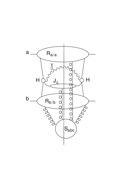
Figure 2: Leading region for prompt photon production near partonic threshold. The vertical line represents the final state, including the photon, $\gamma$, and the recoil jet, $J_{c}$.

The role of the final state jet $J_{c}$ in threshold resummation is well-understood, and has been treated in Refs. [32, 33, 26]. The outgoing jet may interact with soft radiation, through subdiagram $S_{abc}$ in Fig. 2. We may think of the soft function as associated with coherent soft radiation, describing emission and absorption by sources with specified four-velocities and color charges. The role of soft gluon functions encountered in threshold resummation has been extensively studied elsewhere [51]. We will give a formal definition of the fully factorized soft function in subsection 4.3.

There is a potential complication for the joint resummation of the single-photon cross section in the influence of soft radiation on the recoil transverse momentum ${\bf Q}_{T}$ of the photon-$J_{c}$ pair. By analogy to electroweak annihilation, we seek to resum logarithms of $1-\hat{x}_{T}^{2}$ as well as logarithms of the total transverse momentum of the partons involved in the underlying $2\to 2$ hard scattering, ${\bf Q}_{T}$. This transverse momentum is defined relative to the (initial-state) hadronic center-of-mass system, evaluated at fixed observed photon transverse momentum, ${\bf p}_{T}$, in that frame. Referring to Fig. 2, we must ask, however, whether ${\bf Q}_{T}$ is the same on both sides of the cut, i.e., for the amplitude and for its complex conjugate. An imbalance in the relative transverse momenta of the two hard-scatterings would make it necessary to introduce a more complicated convolution than in Eq. (9). Such an imbalance, however, can arise only from the transverse momentum that flows through the soft function $S_{abc}$ between the incoming jet subdiagrams ${\cal R}_{f/f}$ and the outgoing recoil jet $J_{c}$. In the absence of such a flow, the transverse momentum of the final-state jet is a dependent quantity, and does not appear directly in the transverse momentum logarithms. More importantly, a single ${\bf Q}_{T}$ describes the relative transverse momenta of the hard scattering on both sides of the cut.

We must therefore study the flow of transverse momentum through the soft subdiagram. We begin with diagrams that have initial-state interactions only, in which soft gluons, as in electroweak annihilation, couple only to the initial-state jets, ${\cal R}_{a/a}$ and ${\cal R}_{b/b}$ in Fig. 2. The transverse momentum that they carry into the final state must come from the hard scattering, through the initial-state partons, $a$ and $b$, equally in both the amplitude and the complex conjugate amplitude, that is, with the same ${\bf Q}_{T}$ on the two sides of the cut diagram of Fig. 2. At the same time, infrared divergences associated with coherent soft gluons cancel as we sum over different cut diagrams, with different connections of soft gluons to the jet diagrams. In the diagrams necessary to cancel infrared divergences, therefore, the initial-state parton transverse momenta ${\bf k}_{a}$ and ${\bf k}_{b}$ will each vary. Examples are shown in Fig. 3a. This imperfect match means that the cancellation proceeds through plus distributions in ${\bf k}_{a}^{2}$ and ${\bf k}_{b}^{2}$, and can produce logarithms of ${\bf b}$ in the impact parameter space conjugate to ${\bf Q}_{T}$. These purely initial-state interactions can be treated exactly as in Sec. 2 above.

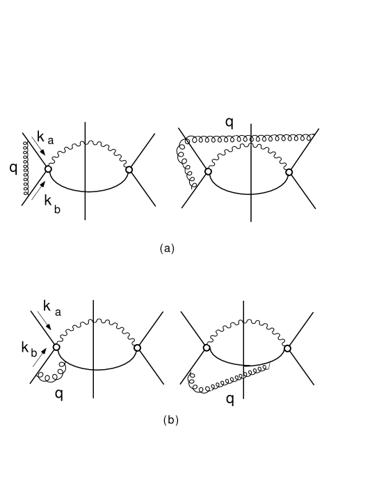
Figure 3: Diagrams that illustrate the cancellation of infrared divergences: (a) initial-state interactions, which require different diagrams, with different parton momenta ${\bf k}_{a}$ and ${\bf k}_{b}$. (b) initial-final-state interference, for which the cancellation proceeds through cuts of a single diagram, at fixed ${\bf k}_{a}$ and ${\bf k}_{b}$.

Consider next soft connections to the final-state jet, including interference between initial- and final-state interactions, as in Fig. 3b, where the soft function $S_{abc}$ now has contributions in which soft radiation is emitted by an initial state line, and absorbed by the final state jet. As usual, we must sum over final states to cancel the infrared divergences associated with this soft radiation. There is, however, a crucial difference between the cancellation of initial-state and initial-final coherent soft radiation. In the case of initial-state radiation, as just described, we must sum over different diagrams to effect the cancellation. Final-state, and initial-final-state interference divergences, however, cancel in the sum over cuts of individual uncut diagrams, as discussed in context of factorization proofs in [50]. Li and Lai also observed that the $k_{T}$-dependence due to final state interactions cancels in the context of prompt photon production [17]. Hence, unlike singularities that arise from purely initial-state interactions, the cancellation of final-state singularities can be effected at fixed transverse momentum for all lines in a cut diagram, in particular, for fixed pair transverse momentum ${\bf Q}_{T}$ of the initial-state partons $a$ and $b$, and hence for the short-distance process in both the amplitude and its complex conjugate. In contrast to initial-state interactions, the transverse-momentum dependence of the final-state soft radiation cancels algebraically, rather than through plus distributions.

It is worth noting that the above result requires that we resum logarithms of the transverse momentum at the short-distance scattering, rather than of the observed photon-jet pair in the final state. In the latter case, the transverse momentum at the short-distance scattering depends on which of the soft gluons attached to the final-state jet are virtual and which are real, and the cancellation of final state infrared divergences reverts from algebra [50] to plus distributions, and may produce logarithms in impact parameter space. When the recoil jet is observed independently, therefore, a somewhat different analysis is necessary, which we shall not carry out here.

To summarize our considerations so far, only the transverse momenta of coherent soft radiation associated with initial-state hard partons must be taken into account in joint resummation. In contrast, final-state and coherent soft radiation linking the outgoing jet with one or both of the incoming jets produces no logarithms in the pair transverse momentum.

The cancellation between the final states in Fig. 3b still requires an integral over energy [1, 4]. For this reason, both initial- and final-state interactions contribute logarithms to threshold resummation. We must incorporate the distinction between initial-state and initial-final interference logarithms into the refactorized convolution that generalizes Eq. (9) for electroweak annihilation to the case of prompt photons. In the next subsection, we show that it is possible to do this by separating purely initial-state soft radiation from initial-final interference, at least to the level of next-to-leading logarithms in both threshold and pair transverse momenta.

4.3. The soft function

To derive an analog of the electroweak annihilation refactorization formula, Eq. (9), for direct photon production, it is necessary to identify a function that summarizes final-state soft gluon radiation. In particular, we want to separate those effects associated with initial-state radiation, which are sensitive to transverse momenta, from those from the final state, which are not. In this subsection, we will construct such a function.

The soft function will be built from nonabelian phase operators, following the discussion of Sec. 2.3 above. We begin by generalizing Eq. (20), which describes the annihilation of a pair of phase operators to a product that corresponds to the color flow [30, 31, 51] at the hard scattering, for the partonic process, $a+b\to\gamma+c$:

$$\left[\,{\cal W}_{abc}(X)\,\right]_{e_{c};e_{b},e_{a}} = \left[\,\Phi^{(c)}_{\beta_{c}}{}(\infty,0;X)\,\right]_{e_{c},d_{c}}\;\left(\,c_{abc}\,\right)_{d_{c};d_{b},d_{a}}$$ (67)

$$\hskip 14.22636pt\times\left[\,\Phi^{(b)}_{\beta_{b}}(0,-\infty;X)\,\right]_{d_{b},e_{b}}\;\left[\,\Phi^{(a)}_{\beta_{a}}(0,-\infty;X)\,\right]_{d_{a},e_{a}}\,.$$

As in Sec. 2.3, we go on construct an eikonal cross section in the form of Eq. (21), at fixed soft-gluon energy, parameterized as $w_{s}Q$, and fixed transverse momentum ${\bf k}$ [30, 34],

$$\sigma^{\rm(eik)}_{abc}(w_{s},Q,{\bf k},\mu,\epsilon) = Q\,\int{d\lambda\over 2\pi}\;{d^{2}{\bf b}\over(2\pi)^{2}}\ {\rm e}^{-i\lambda w_{s}Q+i{\bf b}\cdot{\bf k}}\;$$ (68)

$$\times{1\over C_{A}C_{F}}\,{\rm Tr}\ \langle 0|\,{\rm\bar{T}}\,\left[{\cal W}_{abc}^{\dagger}(0)\right]\,{\rm T}\left[{\cal W}_{abc}(\lambda\hat{n}+{\bf b})\right]\,|0\rangle\,,$$

where the trace is over the external color indices ($e_{i}$) of the operators. In this expression, $\hat{n}$ is the unit vector in the time direction, and we leave the renormalization scale $\mu$ free. The relevant transforms with respect to $w_{s}$ and ${\bf k}$ are Laplace and Fourier, respectively,

$$\bar{\sigma}^{{\rm(eik)}}_{abc}\left({N\mu\over Q},{\bf b}Q,\epsilon\right)=\int_{0}^{\infty}dw_{s}\;{\rm e}^{-Nw_{s}}\,\int{d^{2}{\bf k}}\,{\rm e}^{-i{\bf b}\cdot{\bf k}}\ \sigma^{\rm(eik)}_{abc}(w_{s},Q,{\bf k},\mu,\epsilon)\,.$$ (69)

The soft radiation function for the $a+b\to\gamma+c$ subprocess in prompt photon production is now constructed from $\bar{\sigma}^{{\rm(eik)}}(N,{\bf b})$, by analogy to the soft function $U$ for electroweak annihilation, Eq. (37).

We find the soft function by dividing the transformed eikonal cross section (69) by functions that eliminate double counting with the external jets near partonic threshold: both incoming, and, in this case, outgoing. For the incoming lines, these functions are the $\bar{\cal R}_{a}^{\rm(eik)}(N,{\bf b})$, defined in Eq. (30). Similarly, for the outgoing jet, we identify a new partonic function, which will appear in the refactorization formula, along with its eikonal partner. As we have seen, infrared divergences associated with final state interactions cancel at fixed recoil for the hard scattering. We may therefore treat the outgoing jet inclusively in its transverse momentum. The relevant functions are then the same as those encountered in pure threshold resummation [34]. For example, for a quark jet they may be defined as two-point functions,

$$\tilde{J}_{c}^{\rm(eik)}(N\mu/Q) = \int dw_{c}\;{\rm e}^{-Nw_{c}}\;\int d\sigma\;{\rm e}^{-i(w_{c}Q/\sqrt{2})\sigma}$$

$$\hskip 28.45274pt\times\ {1\over N_{C}}\ {\rm Tr}\langle 0|\Phi^{(q)}_{\beta_{c}}{}^{\dagger}(0)\ \Phi^{(q)}_{\beta_{c}}{}(\sigma\beta_{c})|0\rangle\ \;,$$

$$\tilde{J}_{c}(N\mu/Q,Q/\mu) = \int dw_{c}\;{\rm e}^{-Nw_{c}}\ \int d\lambda d\sigma\;{d^{2}{\bf y}\over(2\pi)^{2}}{\rm e}^{-i(Q/\sqrt{2})\lambda-i(w_{c}Q/\sqrt{2})\sigma}$$ (70)

$$\hskip 14.22636pt\times\ {\pi Q\over\sqrt{2}N_{C}}\;{\rm Tr}\langle 0|q_{c}(0)\;\gamma\cdot\bar{\beta}_{c}\;\bar{q}_{c}(\lambda\bar{\beta}_{c}+\sigma\beta_{c}+{\bf y})|0\rangle$$

$$\equiv \int dw_{c}\;{\rm e}^{-Nw_{c}}\;J_{c}(w_{c},Q)\;,$$

for the eikonal and partonic jet, respectively. In the partonic jet function, $\beta_{c}$ is the light-like velocity vector in the direction of the jet, and $\bar{\beta}_{c}$ is the velocity vector opposite to $\beta_{c}$ in the overall partonic center-of-mass. The matrix elements are evaluated in $n\cdot A=0$ gauge. The traces refer to color and Dirac indices. Outgoing gluon jets may be defined analogously, with operators similar to those used for fragmentation functions [29]. In momentum space, $w_{c}Q^{2}$ is the squared invariant mass of the outgoing jet.

The above reasoning leads to the following generalization of the soft function to prompt photon processes:

$$\bar{S}^{(ab\to\gamma c)}\left({Q\over N\mu},{\bf b}Q,\alpha_{s}(\mu),n\right)={\bar{\sigma}^{{\rm(eik)}}_{abc}\left({Q\over N\mu},{\bf b},\alpha_{s}(\mu),\epsilon\right)\over\bar{\cal R}_{a}^{\rm(eik)}(N\mu/Q,{\bf b}Q,\epsilon)\,\bar{\cal R}_{b}^{\rm(eik)}(N\mu/Q,{\bf b}Q,\epsilon)\,\tilde{J}_{c}^{\rm(eik)}(N\mu/Q)}\,.$$ (71)

As in the case of electroweak annihilation, Eq. (37), this expression is a rewriting of the refactorization of the eikonal cross section into incoming and outgoing jets and soft radiation. Again, the ${\cal R}_{a,b}^{\rm(eik)}$ remove initial-state eikonal radiation from $\hat{\sigma}_{abc}^{\rm(eik)}$, and $\tilde{J}_{c}^{\rm(eik)}(N)$ removes dependence on the outgoing jet. In this form, however, the soft function inherits the gauge dependence implicit in Eq. (71) of the incoming and outgoing jet functions. We can eliminate this dependence, and simplify the overall formalism, by following an observation made in Refs. [30, 51] and employed in [32]. We define a variant soft function in transform space by dividing $\bar{S}$ by a factor $\bar{U}_{i\bar{i}}^{1/2}(N\mu/Q,{\bf b}Q)$ for each of the incoming jets $a$ and $b$, and by $\bar{U}_{c\bar{c}}^{1/2}(N,{\bf 0})$ for the outgoing jet,

$$\bar{S}^{\prime}{}^{(ab\to\gamma c)}\left({Q\over N\mu},{\bf b}Q,\alpha_{s}(\mu)\right) =$$ (72)

$${\bar{S}^{(ab\to\gamma c)}\left({Q\over N\mu},{\bf b}Q,\alpha_{s}(\mu),n\right)\over\bar{U}_{a\bar{a}}^{1/2}(N\mu/Q,{\bf b}Q)\,\bar{U}_{b\bar{b}}^{1/2}(N\mu/Q,{\bf b}Q)\,\bar{U}_{c\bar{c}}^{1/2}(N\mu/Q,{\bf 0})}\,.$$

By shifting factors of $\bar{U}^{1/2}$ from the soft radiation function to the jets in transform space, we produce slightly modified jet functions, of the convolution form

$${\cal R}_{a/a}^{\prime}(x,Q,{\bf k},\epsilon) = \int dwdy\;\delta(w+y-x)\int d{\bf k}_{r}d{\bf k}_{u}\ \delta^{2}({\bf k}_{r}+{\bf k}_{u}+{\bf k})$$

$$\hskip 85.35826pt\times\ {\cal R}_{a/a}(w,Q,{\bf k}_{r},\epsilon)U_{a\bar{a}}^{1/2}(y,Q,{\bf k}_{u})$$

$$= \int_{x}^{1}d\xi\ \phi_{a/a}(\xi,\mu)\,\tilde{c}_{a/a}\left({x\over\xi},{\bf k},Q,\mu\right)+{\cal O}(1/N)\,,$$

$$J^{\prime}_{c}(w_{c},Q) = \int dw^{\prime}dw_{u}\delta(w^{\prime}+w_{u}-w_{c})\ J_{c}(w^{\prime},Q)\;\int d{\bf k}_{u}\;U_{c\bar{c}}^{1/2}(w_{u},{\bf k}_{u})\,,$$ (73)

where in the second equality for ${\cal R}_{a/a}^{\prime}$, $\bar{c}_{a/a}$ is the double inverse transform of the infrared safe function $\bar{c}_{a/a}$ defined in Eq. (34) above.

4.4. Refactorization, recoil and the resummed cross section

The refactorization formula for prompt photon production generalizes the corresponding expression for electroweak annihilation, Eq. (9), by including the outgoing jet function $J_{c}^{\prime}$ in Eq. (73), and the modified soft radiation function $S^{\prime}$, Eq. (72). In transform space the refactorization is in terms of products; in momentum space in terms of convolutions,

$$p_{T}^{3}\;{d\sigma_{ab\to c\gamma}^{({\rm resum})}\over dQ^{2}\,d^{2}{\bf Q}_{T}\,dp_{T}} = \int dx_{a}d^{2}{\bf k}_{a}\,{\cal R}^{\prime}_{a/a}(x_{a},{\bf k}_{a},Q)\;\int dx_{b}d^{2}{\bf k}_{b}\,{\cal R}^{\prime}_{b/b}(x_{b},{\bf k}_{b},Q)$$ (74)

$$\times\;\int dw_{c}\;J^{\prime}_{c}(w_{c},Q)\;\int dw_{s}\,\int d^{2}{\bf k}_{s}\ S^{\prime}{}^{(ab\to\gamma c)}\left(w_{s},Q,{\bf k}_{s},\alpha_{s}(\mu)\right)$$

$$\times\;{1\over S}\ \delta(1-Q^{2}/S-(1-x_{a})-(1-x_{b})-w_{s}-w_{c})\;\delta^{2}\left({\bf Q}_{T}+{\bf k}_{a}+{\bf k}_{b}\right)$$

$$\times\;C_{\delta}^{ab\to\gamma c}(\alpha_{s}(\mu),\tilde{x}_{T}^{2})\;p_{T}^{3}\;{dp_{T}^{\prime}\over dp_{T}}\;{d\hat{\sigma}_{ab\to c\gamma}^{(0)}(\tilde{x}_{T}^{2})\over dp^{\prime}_{T}}\,.$$

Eq. (74) generates, order-by-order in perturbation theory, the same singularities at ${\bf Q}_{T}=0$ as the full cross section, to leading power in $1-Q^{2}/S$. The factor $dp_{T}^{\prime}/dp_{T}$ compensates for the difference in phase space between fixing $p_{T}$ and $p_{T}{}^{\prime}$. The function $C_{\delta}^{(ab\to\gamma c)}=1+{\cal O}(\alpha_{s})$, times the Born cross section, is the perturbative short-distance function, which in the case of prompt photon production (as opposed to electroweak annihilation) depends on $\tilde{x}_{T}^{2}$.  This means that, beyond the lowest order, the short-distance scattering function need not have the same angular dependence as the Born cross section. The short-distance function contains only corrections from (virtual) lines that are off-shell by at least ${\cal O}(p_{T})$. It contains no real-gluon emission, since all radiation has, to leading power in $1-Q^{2}/S$, been absorbed into the long-distance functions ${\cal R}^{\prime}$, $J_{c}^{\prime}$ and $S^{\prime}$. The computation of these short-distance functions is equivalent to the matching conditions of effective field theories.

With $S^{\prime}$ constructed as above, the soft transverse momentum ${\bf k}_{s}$ is associated entirely with final-state interactions, and is not included in the recoil momentum of the hard subprocess. We may therefore integrate over ${\bf k}_{s}$ and redefine

$$S^{\prime}{}^{(ab\to\gamma c)}\left(w_{s},Q,\alpha_{s}(\mu)\right)\equiv\int d^{2}{\bf k}_{s}\ S^{\prime}{}^{(ab\to\gamma c)}\left(w_{s},Q,{\bf k}_{s},\alpha_{s}(\mu)\right)\,,$$ (75)

where on the left we retain the same notation for the function, but omit the transverse argument. Our refactorization formula then simplifies to

$$p_{T}^{3}\;{d\sigma_{ab\to c\gamma}^{({\rm resum})}\over dQ^{2}\,d^{2}{\bf Q}_{T}\,dp_{T}} = \int dx_{a}d^{2}{\bf k}_{a}\,{\cal R}^{\prime}_{a/a}(x_{a},{\bf k}_{a},Q)\;\int dx_{b}d^{2}{\bf k}_{b}\,{\cal R}^{\prime}_{b/b}(x_{b},{\bf k}_{b},Q)$$ (76)

$$\times\;\int dw_{c}\;J^{\prime}_{c}(w_{c},Q)\;\int dw_{s}S^{\prime}{}^{(ab\to\gamma c)}\left(w_{s},Q,\alpha_{s}(\mu)\right)$$

$$\times\;{1\over S}\ \delta(1-Q^{2}/S-(1-x_{a})-(1-x_{b})-w_{s}-w_{c})$$

$$\times\;\delta^{2}\left({\bf Q}_{T}+{\bf k}_{a}+{\bf k}_{b}\right)$$

$$\times\;C_{\delta}^{(ab\to\gamma c)}(\alpha_{s}(\mu),\tilde{x}_{T}^{2})\;p_{T}^{3}\;{dp_{T}^{\prime}\over dp_{T}}\;{d\hat{\sigma}_{ab\to c\gamma}^{(0)}(\tilde{x}_{T}^{2})\over dp^{\prime}_{T}}\,.$$

To simplify the notation further, we also introduce a new function ${\cal F}$, which combines contributions from the final-state jet and soft final-state radiation,

$${\cal F}_{abc}(w_{f})=\int dw_{s}dw_{c}\,S^{\prime}{}^{(ab\to\gamma c)}\left(w_{s},Q,\alpha_{s}(\mu)\right)\;J_{c}^{\prime}(w_{c},Q)\ \delta\left(w_{f}-w_{s}-w_{c}\right)\,.$$ (77)

As described above, this convolution does not involve the recoil transverse momentum. In moment space, Eq. (77) becomes a product

$$\tilde{\cal F}_{abc}(N)=\tilde{S}^{\prime}{}^{(ab\to\gamma c)}\left({Q\over N\mu}\right)\,\tilde{J}_{c}^{\prime}(N)+{\cal O}(1/N)\,.$$ (78)

We will discuss the explicit $N$-dependence from soft gluon radiation and the final-state jet below.

Eq. (76) defines recoil in the prompt photon cross section in much the same way that Eq. (9) defines it for electroweak annihilation. The short distance functions, $C_{\delta}\;d\sigma^{(0)}(\tilde{x}_{T}^{2})/dp_{T}$ include only lines off-shell by ${\cal O}(p_{T}^{\prime}{}^{2})$, and are evaluated at zero relative transverse momenta for initial-state partons. Expansions in the transverse momenta of the incoming partons are to be absorbed into higher orders in $C_{\delta}$. In this convolution form, however, the kinematics of the hard scattering influences the cancellation of singularities at vanishing ${\bf k}_{a}$ and ${\bf k}_{b}$. This procedure has a straightforward interpretation order-by-order. At fixed order, all contributions that are singular at threshold for fixed $Q^{2}$ may be put in the form of Eq. (76). To evaluate the cross section at any fixed order, we would integrate each such contribution over $Q^{2}$ and ${\bf Q}_{T}$, as in Eq. (66), with no further approximations. The result would contain finite corrections resulting from the kinematic linkage of the hard scattering with the cancellation of singularities in transverse momentum. We would then sum to all orders. In the resummed formalism, we simply approximate the short-distance function to ${\cal O}(\alpha_{s})$, sum the singularities to all orders at leading or next-to-leading logarithmic accuracy, and do the $Q^{2}$ and ${\bf Q}_{T}$ integrals last. In the following, we shall derive the consequences of this reorganization of perturbation theory.

We are now ready to return to Eq. (66), and derive the jointly-resummed partonic cross section as an integral of the differential resummed cross section (76) over the hard-scattering scale $Q$ and its relative transverse momentum, ${\bf Q}_{T}$. Changing variables from $Q^{2}$ to $\tilde{x}_{T}^{2}$, we derive

$${p_{T}^{3}d\sigma^{({\rm resum})}_{ab\to\gamma}\over dp_{T}} = \frac{p_{T}^{4}}{8\pi S^{2}}\ \sum_{ij}\;\int_{0}^{1}d\xi_{i}\;d\xi_{j}\;{\phi}_{i/a}(\xi_{i},\mu){\phi}_{j/b}(\xi_{j},\mu)$$ (79)

$$\times\;\int d^{2}{\bf Q}_{T}\;\theta\left(\bar{\mu}-|{\bf Q}_{T}|\right)\;\int_{0}^{1}d\tilde{x}^{2}_{T}\;{|M_{ij}(\tilde{x}^{2}_{T})|^{2}\over\sqrt{1-\tilde{x}_{T}^{2}}}\;C_{\delta}^{(ij\to\gamma k)}(\alpha_{s}(\mu),\tilde{x}_{T}^{2})$$

$$\times\;\int d^{2}{\bf k}_{i}\;d^{2}{\bf k}_{j}\;\delta^{2}\left({\bf Q}_{T}+{\bf k}_{i}+{\bf k}_{j}\right)\,\int_{0}^{\xi_{i}}dx_{i}\,\int_{0}^{\xi_{j}}dx_{j}\,\int_{0}^{1}dx_{f}\,\delta\left(\tilde{x}_{T}^{2}-\left({{p}_{T}^{\prime}{}^{2}\over p_{T}^{2}}\right)\,{x_{T}^{2}\over x_{i}x_{j}(1-x_{f})}\right)$$

$$\times\;\bar{c}_{i/i}\left({x_{i}\over\xi_{i}},{\bf k}_{i},\frac{2p^{\prime}_{T}{}}{\tilde{x}_{T}},\mu\right)\bar{c}_{j/j}\left({x_{j}\over\xi_{j}},{\bf k}_{j},\frac{2p^{\prime}_{T}{}}{\tilde{x}_{T}},\mu\right){\cal F}_{ijk}(x_{f},\tilde{x}_{T}^{2})\,\left({1\over x_{i}x_{j}(1-x_{f})}\right)^{2}\,,$$

where we have used Eq. (73) to isolate the partonic hard-scattering function in $\overline{\rm MS}$ scheme, and Eq. (77) to summarize the contribution of soft and jet radiation in the final state. In the argument of the delta function, we have used Eq. (64) to reexpress the ratio $Q^{2}/S$ as

$${Q^{2}\over S}=\left({p_{T}^{\prime}{}^{2}\over p_{T}^{2}}\right){x_{T}^{2}\over\tilde{x}_{T}^{2}}\,.$$ (80)

In Eq. (79), we have also reexpressed the Born cross sections in terms of the $2\to 2$ invariant amplitudes $M(\tilde{x}_{T}^{2})$, and have used the approximate relation $p_{T}^{\prime}(dp_{T}^{\prime}/dp_{T})=p_{T}$, valid up to a nonsingular term of ${\cal O}({\bf Q}_{T})$, which we neglect.

It is a relatively small step from Eq. (79) to a jointly resummed cross section for hadrons, by replacing partonic by hadronic $\overline{\rm MS}$ distributions,

$${p_{T}^{3}d\sigma^{({\rm resum})}_{AB\to\gamma}\over dp_{T}} = \frac{p_{T}^{4}}{8\pi S^{2}}\ \sum_{ij}\;\int_{0}^{1}d\xi_{i}\;d\xi_{j}\;{\phi}_{i/A}(\xi_{i},\mu){\phi}_{j/B}(\xi_{j},\mu)$$ (81)

$$\times\;\int{d^{2}{\bf Q}_{T}\over(2\pi)^{2}}\;\theta\left(\bar{\mu}-|{\bf Q}_{T}|\right)\;\int_{0}^{1}d\tilde{x}^{2}_{T}\;{|M_{ij}(\tilde{x}^{2}_{T})|^{2}\over\sqrt{1-\tilde{x}_{T}^{2}}}\;C_{\delta}^{(ij\to\gamma k)}(\alpha_{s}(\mu),\tilde{x}_{T}^{2})$$

$$\times\;\int d^{2}{\bf b}\;{\rm e}^{i{\bf b}\cdot{\bf Q}_{T}}\;\left({S\over 2{p}^{\prime}_{T}{}^{2}}\right)\;\int_{0}^{\xi_{i}}dx_{i}\,\int_{0}^{\xi_{j}}dx_{j}\,\int_{0}^{1}dx_{f}\,\delta\left(\tilde{x}_{T}^{2}-\left({{p}_{T}^{\prime}{}^{2}\over p_{T}^{2}}\right)\,{x_{T}^{2}\over x_{i}x_{j}(1-x_{f})}\right)$$

$$\times\;\bar{c}_{i/i}\left({x_{i}\over\xi_{i}},{\bf b},\frac{2p^{\prime}_{T}{}}{\tilde{x}_{T}},\mu\right)\bar{c}_{j/j}\left({x_{j}\over\xi_{j}},{\bf b},\frac{2p^{\prime}_{T}{}}{\tilde{x}_{T}},\mu\right){\cal F}_{ijk}(x_{f},\tilde{x}_{T}^{2})\,\left({1\over x_{i}x_{j}(1-x_{f})}\right)^{2}\,,$$

where we have also replaced the convolution in transverse momenta by a Fourier transform, so that the functions $\bar{c}$ are now in impact parameter space.

Eq. (81) factorizes under $x_{T}^{2}$ moments at large $N$, up to $1/N$ corrections. Thus, following essentially the same steps that led to Eq. (43) for electroweak annihilation, we find the physical cross section as an inverse transform [19],

$${p_{T}^{3}d\sigma^{({\rm resum})}_{AB\to\gamma}\over dp_{T}} = \frac{p_{T}^{4}}{8\pi S^{2}}\ \sum_{ij}\ \int_{\cal C}{dN\over 2\pi i}\;\tilde{\phi}_{i/A}(N,\mu)\tilde{\phi}_{j/B}(N,\mu)$$ (82)

$$\times\int_{0}^{1}d\tilde{x}^{2}_{T}\;\left(\tilde{x}^{2}_{T}\right)^{N}{|M_{ij}(\tilde{x}^{2}_{T})|^{2}\over\sqrt{1-\tilde{x}_{T}^{2}}}\;C_{\delta}^{(ij\to\gamma k)}(\alpha_{s}(\mu),\tilde{x}_{T}^{2})$$

$$\times\int{d^{2}{\bf Q}_{T}\over(2\pi)^{2}}\;\theta\left(\bar{\mu}-|{\bf Q}_{T}|\right)\left(\frac{S}{4|{\bf p}_{T}-{\bf Q}_{T}/2|^{2}}\right)^{N+1}$$

$$\times\;\int d^{2}{\bf b}\;{\rm e}^{i{\bf b}\cdot{\bf Q}_{T}}\;\bar{c}_{i/i}\left(N,{\bf b},\frac{4p^{\prime}_{T}{}^{2}}{\tilde{x}^{2}_{T}},\mu\right)\bar{c}_{j/j}\left(N,{\bf b},\frac{4p^{\prime}_{T}{}^{2}}{\tilde{x}^{2}_{T}},\mu\right)\ \tilde{\cal F}_{ijk}(N,\tilde{x}_{T}^{2})\,.$$

In the $\bar{c}$’s, the impact parameter ${\bf b}$ is conjugate to ${\bf Q}_{T}$ at fixed values of $Q^{2}={4p^{\prime}_{T}{}^{2}}/{\tilde{x}^{2}_{T}}$. In this form, however, each $\bar{c}_{i/i}$ also depends implicitly on ${\bf Q}_{T}$, through $p^{\prime}_{T}{}^{2}$. Explicit forms for the functions $\bar{c}_{i/i}$ have been given in Eq. (57) above. In the next subsection, we will find the $N$-dependence of the final-state function $\cal F$.

4.5. Resummation for the final state

Constructed as in Eq. (71), $\tilde{S}^{\prime}{}^{(ab\to\gamma c)}$ satisfies the same renormalization group equation as the soft functions encountered in heavy quark [30] and jet [34] threshold resummations,

$$\mu{d\over d\mu}\,\ln\tilde{S}^{\prime}{}^{(ab\to\gamma c)}\left({Q\over N\mu},\alpha_{s}(\mu)\right)=-2{\rm Re}\,\Gamma^{(ab\to\gamma c)}_{S^{\prime}}(\alpha_{s}(\mu))\;,$$ (83)

where the anomalous dimension $\Gamma^{(ab\to\gamma c)}_{S^{\prime}}$ is a function of the velocities $\beta_{i}$ associated with the phase lines corresponding to partons $a$, $b$ and $c$. For the special case of prompt photon production, $\Gamma_{S^{\prime}}$ is a number, rather than a matrix, because the short-distance cross section has only one color structure [32, 33]. The solution to (83) is therefore a simple exponential,

$$\tilde{S}^{\prime}{}^{(ab\to\gamma c)}\left({Q\over N\mu},\alpha_{s}(\mu)\right) = \tilde{S}^{\prime}{}^{(ab\to\gamma c)}\left(1,\alpha_{s}(Q/N)\right)$$ (84)

$$\hskip 14.22636pt\times\exp\;\left[\int_{\mu}^{Q/N}{d\mu^{\prime}\over\mu^{\prime}}2{\rm Re}\,\Gamma^{(ab\to\gamma c)}_{S^{\prime}}\left(\alpha_{s}(\mu^{\prime})\right)\right]\,.$$

The logarithm of the soft function, constructed in this fashion, has at most a single logarithm of $N$ per loop, so that by calculating $\Gamma^{(ab\to\gamma c)}_{S^{\prime}}$ to one loop, we determine $S^{\prime}{}^{(ab\to\gamma c)}$ at the level of its leading logarithms, that is, $\alpha_{s}^{L}\ln^{L}N$ in the exponent, while remaining at NLL in the overall cross section.

Figure 4: (a) Diagrams which contribute to the soft anomalous dimension. The crosses on the gluon lines denote the modified propagator given in the text. The remainder of the $A^{0}=0$ gauge propagator cancels the real part of (b).

$\Gamma^{(ab\to\gamma c)}_{S^{\prime}}$ is calculated from the $\overline{\rm MS}$ counterterms for the three diagrams shown in Fig. 4, in which a single gluon is exchanged between pairs of eikonals. The details of these calculations, which are to be carried out in an axial $n\cdot A=0$ gauge, are described in [51]. Many terms cancel, and in Fig. 4a, the additional crosses on the gluon lines denote a slightly modified $A^{0}=0$ gauge propagator:

$${1\over k^{2}}\,\left(\,-g^{\mu\nu}+{\hat{n}^{\mu}k^{\nu}+k^{\mu}\hat{n}^{\nu}\over\hat{n}\cdot k}-{1\over 2}{k^{\mu}k^{\nu}\over(\hat{n}\cdot k)^{2}}\right)\,.$$ (85)

The factor $1/2$ in this expression is specific to the lowest-order calculation. It takes into account the effect of subtracting the factor $U_{a\bar{a}}U_{b\bar{b}}$ implicit in the definition of $c_{a}c_{b}$, Eq. (34). The “missing” terms in Eq. (85) completely cancel the real part of the diagram of Fig. 4b. The resulting anomalous dimension is then

$${\rm Re}\,\Gamma^{(q\bar{q}\to\gamma g)}_{S^{\prime}} = {\alpha_{s}\over 2\pi}\,C_{A}\,\ln\left({tu\over s^{2}}\right)$$

$${\rm Re}\,\Gamma^{(qg\to\gamma g)}_{S^{\prime}} = {\alpha_{s}\over 2\pi}\,\left[\;2C_{F}\,\ln\left({-u\over s}\right)+C_{A}\,\ln\left({t\over u}\right)\;\right]\,,$$ (86)

where $s$, $t$ and $u$ are the invariants for the partonic $2\to 2$ subprocess. These anomalous dimensions are independent of the gauge vector $n^{\mu}$ at one loop [51]. The functions $S^{\prime}{}^{(ab\to\gamma c)}$, defined as the solutions to Eq. (83), with the usual boundary condition $S^{\prime}{}^{(ab\to\gamma c)}(N=0)=1$, are free of initial-state radiation that would be sensitive to recoil at the logarithmic level. They continue to contribute to the threshold phase space through the energy $w_{s}Q$ [30, 34], in a manner described below.

Explicit expressions for $\tilde{S}^{\prime}(N)$ are found from Eqs. (84) and (86) above. The transform of the recoil jet function may be found from Ref. [52], and is given in its most general form by

$$\tilde{J}^{\prime}_{c}(N) = \exp[\,E^{\prime}_{c}(N)\,]$$

$$E^{\prime}_{c}(N) = \int^{1}_{0}dz\frac{z^{N-1}-1}{1-z}\;\left\{\int^{(1-z)}_{(1-z)^{2}}\frac{d\lambda}{\lambda}A_{c}\left[\alpha_{s}(\sqrt{\lambda}Q)\right]\right.$$ (87)

$$\hskip 56.9055pt\left.{}+B^{\prime}_{c}\left[\alpha_{s}(\sqrt{1-z}Q)\right]+B^{\prime\prime}_{c}\left[\alpha_{s}((1-z)Q)\right]\right\}\,,$$

where the $A_{c}$ are given in Eq. (15). In the specific normalization chosen for the recoil jet, $J^{\prime}_{c}$, in Eq. (73) above, $B_{c}^{\prime}{}^{\prime}$ vanishes, while

$$B^{\prime}_{q}=\frac{\alpha_{s}}{\pi}\left(-\frac{3}{4}\right)C_{F}\,,\quad B^{\prime}_{g}=\frac{\alpha_{s}}{\pi}\left(-{\beta_{0}\over 4}\right)\,.$$ (88)

These results, along with Eq. (57) for the functions $\tilde{c}_{i/i}$, specify the explicit NLL resummed cross section as an inverse Mellin moment in Eq. (82). We will give the relevant expressions in Sec. 5. We close this section with a discussion of the additional considerations necessary to include fragmentation effects in the formalism.

4.6. Including fragmentation

For single-particle inclusive hadron production, and even for high-$p_{T}$ photon production, we must supplement the considerations above to include final-state fragmentation. This is relatively easy, since the dynamics of fragmentation factorizes from initial-state, hard virtual, and soft coherent radiation as well as from the final-state corrections associated with the recoiling jet, as illustrated in Fig. 5. The analysis of this section applies to pure threshold resummation (as discussed in [26]) as well as to joint resummation.

The underlying short-distance scattering subprocess is again a $2\to 2$ reaction, but now with two outgoing colored particles, one of which fragments into the observed hadron, which we may take to be a pion (or photon):

$$a(x_{a}p_{a})+b(x_{b}p_{b})\to c+d(P/z)\to\pi(P)+X\,,$$ (89)

where we have exhibited the partons’ momenta. The outgoing jet, $J_{d}$, fragments into the observed hadron ($\pi$). The short-distance scattering involves more than one color flow, the set depending on the flavors of the partons in Eq. (89). At any order in perturbation theory, the color flow in the amplitude and complex conjugate need not be the same. Referring to Fig. 5, and adopting the notation of electroweak annihilation, we represent the (dimensionless) short-distance function as $p_{T}^{3}\;{d\hat{\sigma}_{JI}^{\rm(f)}(\tilde{x}_{T}^{2})/dp^{\prime}_{T}}=h^{*}_{J}\;h_{I}$, where f denotes the $2\to 2$ partonic scattering of Eq. (89). The soft function is built in the same way as for prompt photon production, treating the color tensors $c_{I,J}$ for each color exchange at the hard scattering as an effective local vertex linking phase operators in the flavors of the partons $a\dots d$. The soft function is written as $S_{JI}^{\rm(f)}$. The same arguments regarding the cancellation of recoil effects in the soft function apply to single-hadron inclusive as to prompt photon production. Also, the normalization of the soft function follows Eq. (72) above, for each of the matrix elements of $S^{\rm(f)}_{JI}$, but now with factors $U^{1/2}$ for both outgoing jets. The resulting anomalous dimensions for most relevant flavor flows have been computed in Refs. [30, 51].

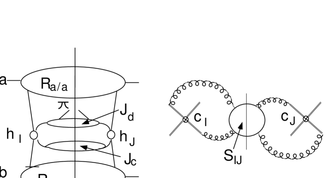
Figure 5: Leading region for a single-particle inclusive cross section in cut diagram form. $c_{I}$ and $c_{J}$ represent color tensors [51].

Near threshold, in the notation of Eqs. (74) and (80), the phase space is slightly modified, relative to the prompt photon case, because the fragmenting jet has invariant mass $q_{d}^{2}\geq 0$, and because the outgoing parton at the hard scattering carries momentum $P/z\geq P$, which shifts the scaling variable $\tilde{x}_{T}$ by a factor $z$. This changes the transverse momentum in the hard-scattering center-of-mass system: ${\bf p}_{T}^{\prime}\to{\bf p}^{\prime}{}^{\prime}_{T}(z)\equiv{\bf p}_{T}/z-{\bf Q}_{T}/2$, which is related to the short-distance scattering and overall invariant masses squared, $Q^{2}$ and $S$, by

$${Q^{2}\over S}=\left({|{\bf p}^{\prime}{}^{\prime}_{T}|^{2}\over|{\bf p}_{T}|^{2}}\right){x_{T}^{2}\over\tilde{x}_{T}^{2}}\sim\left({|{\bf p}^{\prime}_{T}|^{2}\over|{\bf p}_{T}|^{2}}\right){x_{T}^{2}\over z^{2}\tilde{x}_{T}^{2}}\,.$$ (90)

In the second relation we have expanded in $1-z$, and have neglected corrections of the form $(1-z){\bf Q}_{T}$. In place of the argument of the first delta function in Eq. (74) for resummed prompt photon production, we find the following kinematic constraint near partonic threshold for single-particle inclusive cross sections with fragmentation:

$$1 = {Q^{2}\over S}+(1-x_{a})+(1-x_{b})+w_{s}+q_{c}^{2}/S+q_{d}^{2}/S$$ (91)

$$= {|{\bf p}^{\prime}_{T}|^{2}\over|{\bf p}_{T}|^{2}}{x_{T}^{2}\over\tilde{x}_{T}^{2}}+2(1-z)+(1-x_{a})+(1-x_{b})+w_{s}+q_{c}^{2}/S+q_{d}^{2}/S\,,$$

with $x_{T}^{2}$ as in Eq. (59) and $\tilde{x}_{T}^{2}$ as in (63).

The refactorization that generalizes Eq. (74) includes an additional integral over $z$, linked through the restriction (91), and a function that describes the fragmentation of parton $d$ into hadron $\pi(P)$. We parameterize the momentum of parton $d$ as

$$q_{d}^{\mu}={P^{\mu}\over z}+\left({z\;q_{d}^{2}\over 2P\cdot\bar{\beta}_{d}}\right)\,\bar{\beta}_{d}^{\mu}\equiv\frac{P\cdot\bar{\beta}_{d}}{z}\beta_{d}^{\mu}+\frac{zw_{d}Q^{2}}{2P\cdot\bar{\beta}}\,\bar{\beta}_{d}^{\mu}$$ (92)

where $\bar{\beta}_{d}^{\mu}$ is the opposite-directed unit light-cone vector relative to momentum $P^{\mu}=(P\cdot\bar{\beta}_{d})\beta_{d}^{\mu}$, which is itself taken to be lightlike. The second form introduces a dimensionless variable $w_{d}\equiv q^{2}_{d}/S$.

The fragmentation dynamics of the outgoing jet can be described by a function that is quite similar to a standard fragmentation function [29], and to the inclusive jet functions (70) above. As above, we illustrate the case of a quark $q_{f}$, computed in $n\cdot A=0$ gauge,

$$J_{f/f}(w_{d},P,z,\epsilon) = {Q\over 8N_{C}}\sum_{X}\;\int{d\lambda d\sigma\over 2\pi}\ {\rm e}^{-i(P\cdot\bar{\beta}_{d}/z)\lambda-iq_{d}\cdot\beta_{d}\sigma}$$ (93)

$$\hskip 28.45274pt\times\ {\rm Tr}\;\langle 0|\,q_{f}(0)\,|f(P),X\rangle\,\hbox to0.0pt{/\hss}{\bar{\beta}}_{d}\,\langle f(P),X|\bar{q}_{f}(\lambda\beta_{d}+\sigma\bar{\beta}_{d})\,|0\rangle$$

$$= \int_{z}^{1}{d\xi\over\xi}\ e_{f/f}\left({z\over\xi},{w_{d}},P,\mu_{F}\right)\;D_{f/f}(\xi,\mu_{F},\epsilon)\,,$$

with $\mu_{F}$ a factorization scale. In the first, defining, relation, the trace is over both color and Dirac indices. A sum over spins is understood. In the second equality, $D_{f/f}$ is a fragmentation function, which we may define in $\overline{\rm MS}$ factorization scheme. As usual, at partonic threshold, the infrared-safe coefficient function $e_{d/d}$ may be taken diagonal in flavor, up to corrections that vanish as $1/N$ in moment space.

It is convenient to define a final state threshold function by analogy to Eq. (77), as a convolution of the soft function with the recoiling jet,

$${\cal F}_{JI}^{\rm(f)}\left(w_{f}\right)\equiv\frac{1}{S}\int dw_{s}\,dq_{c}^{2}\,\delta\left(w_{f}-w_{s}-q_{c}^{2}/S\right)\ S_{JI}^{\prime}{}^{\rm(f)}\left(w_{s},Q,\mu\right)\;J^{\prime}_{c}(q_{c}^{2})\,.$$ (94)

Laplace moments reduce the convolution to a product,

$$\tilde{\cal F}_{JI}^{\rm(f)}(N) = \int_{0}^{\infty}dw_{f}\;{\rm e}^{-Nw_{f}}\ {\cal F}_{JI}^{\rm(f)}(w_{f})$$ (95)

$$= \tilde{S}_{JI}^{\prime}{}^{\rm(f)}\left({Q\over N\mu},\alpha_{s}(\mu)\right)\;\tilde{J}^{\prime}_{c}(N)\,.$$

It is now straightforward to generalize each of Eqs. (76), (82) and (81), corresponding to refactorization at partonic threshold, and to the jointly-resummed hadronic cross section written as an inverse moment, and in convolution form, respectively. We give below the first two of these generalized expressions explicitly.

The refactorized partonic single-particle inclusive cross section is given by

$$p_{T}^{3}\;{d\sigma_{\rm f}^{({\rm resum})}\over dQ^{2}\,d^{2}{\bf Q}_{T}\,dp_{T}} = \int dx_{a}d^{2}{\bf k}_{a}\,{\cal R}^{\prime}_{a/a}(x_{a},{\bf k}_{a},Q)\;\int dx_{b}d^{2}{\bf k}_{b}\,{\cal R}^{\prime}_{b/b}(x_{b},{\bf k}_{b},Q)$$ (96)

$$\hskip 28.45274pt\times\;\delta^{2}\left({\bf Q}_{T}+{\bf k}_{a}+{\bf k}_{b}\right)\,\int dz\,\int dw_{d}$$

$$\hskip 28.45274pt\times\;\sum_{IJ}\ \int dw_{f}\;{\cal F}_{JI}^{\rm(f)}\left(w_{f}\right)\;p_{T}^{3}\;{dp_{T}^{\prime}\over dp_{T}}\;{d\hat{\sigma}_{JI}^{\rm(f)}(\tilde{x}_{T}^{2})\over dp^{\prime}_{T}}$$

$$\hskip 28.45274pt\times\;\int_{z}^{1}{d\xi\over\xi}\ e_{d/d}\left({z\over\xi},{w_{d}},P,\mu_{F}\right)\;D_{d/d}(\xi,\mu_{F},\epsilon)\;$$

$$\hskip 28.45274pt\times\;{1\over S}\ \delta\left(1-{Q^{2}/S}-(1-x_{a})-(1-x_{b})-w_{f}-w_{d}\right)\;\,,$$

where $\tilde{x}_{T}$ is specified by Eq. (90). As indicated in Eq. (66), the resummed cross section is found by integrating over $Q^{2}$ and ${\bf Q}_{T}$. The form convenient for $x_{T}^{2}$-moments is found by changing variables from $Q^{2}$ to $\tilde{x}_{T}^{2}$. We compute the hard-scattering cross section in moment space, by dividing by perturbative distributions for the incoming partons, and by a perturbative fragmentation function for the parton that fragments into the observed particle.

The resummed hadronic cross section is found by replacing the perturbative distributions and fragmentation function by their hadronic analogs in moment space, and inverting the transform with respect to $x_{T}^{2}$. The result is

$${p_{T}^{3}d\sigma^{({\rm resum})}_{AB\to\gamma}\over dp_{T}} = \frac{p_{T}^{4}}{8\pi S^{2}}\ \sum_{\rm f}\ \int_{\cal C}{dN\over 2\pi i}\;\tilde{\phi}_{a/A}(N,\mu)\tilde{\phi}_{b/B}(N,\mu)\ \tilde{D}_{\pi/d}(2N+3,\mu)$$

$$\times\int_{0}^{1}d\tilde{x}^{2}_{T}\;\left(\tilde{x}^{2}_{T}\right)^{N}{|M^{(\rm f)}_{IJ}(\tilde{x}^{2}_{T},\alpha_{s}(\mu))|^{2}\over\sqrt{1-\tilde{x}_{T}^{2}}}\;C_{\delta}^{\rm(f)}(\alpha_{s}(\mu),\tilde{x}_{T}^{2})$$

$$\times\int{d^{2}{\bf Q}_{T}\over(2\pi)^{2}}\;\Theta\left(\bar{\mu}-|{\bf Q}_{T}|\right)\left(\frac{S}{4|{\bf p}_{T}-{\bf Q}_{T}/2|^{2}}\right)^{N+1}$$

$$\times\int d^{2}{\bf b}\;{\rm e}^{i{\bf b}\cdot{\bf Q}_{T}}\;\bar{c}_{a/a}\left(N,{\bf b},\frac{4p_{T}^{2}}{\tilde{x}^{2}_{T}},\mu\right)\bar{c}_{b/b}\left(N,{\bf b},\frac{4p_{T}^{2}}{\tilde{x}^{2}_{T}},\mu\right)\ \tilde{\cal F}_{JI}^{\rm(f)}(N,\tilde{x}_{T}^{2})\;\tilde{e}_{d/d}\left(2N+3,N,P,\mu_{F}\right)\,,$$

where we define

$$\tilde{e}_{d/d}\left(M,N,P,\mu_{F}\right)\equiv\int dy\,dw_{d}\ {\rm e}^{-M(1-y)-Nw_{d}}\ e_{d/d}\left(y,w_{d},P,\mu_{F}\right)\,.$$ (98)

In Eq. (4.6.), $M^{\rm(f)}_{IJ}$ denotes the projection of the amplitude squared at lowest nonvanishing order on each of the color flows in the amplitude and complex conjugate, and $C_{\delta}^{\rm(f)}$ is the corresponding expansion in $\alpha_{s}$ of the complete hard-scattering function. A similar form was found in Ref. [26] in the context of threshold resummation for the fragmentation component of high-$p_{T}$ photon production. The function $\tilde{e}_{d/d}$ in Eq. (98) is a double moment, with respect to the jet invariant mass squared, $w_{d}Q^{2}$ and the scaling variable, $y$. Its double logarithmic behavior [26], however, is determined entirely by the latter, because in the momentum configurations that give rise to double logarithms, we have $1-y\gg w_{d}$, corresponding to the collinear emission of soft gluons. Finally, we note once again the dependence of the resummed cross section on a cutoff scale $\bar{\mu}$. At this scale, the resummed cross section must be matched to a finite-order, or partially resummed cross section. The investigation of the best implementation of this procedure remains for future work.

5. Exponents at NLL

In this section we apply joint resummation to electroweak annihilation and prompt photon production, and exhibit the relevant exponents to next-to-leading logarithm. For prompt photons, these expressions were the basis of the phenomenological estimates given in Ref. [19]. We reserve for future work the corresponding results for single-particle annihilation including fragmentation, since they will require slightly more elaborate calculations involving color mixing at the hard scattering [30, 51].

5.1. Electroweak annihilation

Starting from Eq. (56), we can identify an explicit expression for the resummed electroweak annihilation cross section that is accurate to NLL in both $N$ and $b$ [19]. We recall first that the exponent $D_{ab}$ in (56) contributes only at NNLL. For the NLL exponent $E_{ab}$, we have used for guidance the NLL approximation to threshold resummation introduced in Ref. [26]. Our expression for the perturbative exponent $E_{ab}^{\rm PT}$ in Eq. (56) is

$$E_{ab}^{\rm PT}(N,b,Q,Q) = \int_{(b/c_{1}+\bar{N}/Q)^{-1}}^{Q}{d\mu^{\prime}\over\mu^{\prime}}\;\left[\,A_{a}(\alpha_{s}(\mu^{\prime}))+A_{b}(\alpha_{s}(\mu^{\prime}))\,\right]\,\;2\ln{\bar{N}\mu^{\prime}\over Q}\,,$$ (99)

where as above, we define $\bar{N}=N{\rm e}^{\gamma_{E}}$. Eq. (99) approaches the normal forms of $Q_{T}$-resummation (in $b$-space) as $b\to\infty$ at fixed $N$, and of threshold resummation for $N\to\infty$ at fixed $b$. We have introduced an explicit dimensionless scale $c_{1}$ into the $b$-dependence of the lower limit in the first integral. In Eq. (99), the factorization scale, set to $\mu_{F}=Q$ in the upper limit of the integral, replaces the conventional upper limit $c_{2}Q$ in the $Q_{T}$-resummation formalism [8, 9].

Following the format of [26], we find the following closed expression for $E_{a\bar{a}}^{\rm PT}$, accurate to NLL in both $N$ and $b$,

$$E_{a\bar{a}}^{\rm PT}(N,b,Q,\mu_{F})=\frac{2}{\alpha_{s}(\mu)}h_{a}^{(0)}(\lambda,\beta)+2h_{a}^{(1)}(\lambda,\beta,Q,\mu,\mu_{F})\;,$$ (100)

where for $a=q$ or $g$ we define

$$h_{a}^{(0)}(\lambda,\beta) = \frac{A_{a}^{(1)}}{2\pi b_{0}^{2}}\left[2\beta+(1-2\lambda)\ln(1-2\beta)\right]\,,$$ (101)

and

$$h_{a}^{(1)}(\lambda,\beta,Q,\mu,\mu_{F}) = \frac{A_{a}^{(1)}b_{1}}{2\pi b_{0}^{3}}\left[\frac{1}{2}\ln^{2}(1-2\beta)+\frac{1-2\lambda}{1-2\beta}(2\beta+\ln(1-2\beta))\right]$$ (102)

$$+ \frac{1}{2\pi b_{0}}\left(-\frac{A_{a}^{(2)}}{\pi b_{0}}+A_{a}^{(1)}\ln\left(\frac{Q^{2}}{\mu^{2}}\right)\right)\left[2\beta\frac{1-2\lambda}{1-2\beta}+\ln(1-2\beta)\right]$$

$$- \frac{A_{a}^{(1)}}{\pi b_{0}}\lambda\ln\left(\frac{Q^{2}}{\mu_{F}^{2}}\right)\;,$$

in terms of moment variables,

$$\lambda = b_{0}\alpha_{s}(\mu)\ln\left(\bar{N}\right)\;,$$

$$\beta = b_{0}\alpha_{s}(\mu)\ln\left(\bar{N}+bQ/c_{1}\right)\,.$$ (103)

The coefficients $A_{a}^{(1)}$ and $A_{a}^{(2)}$ in Eqs. (101) and (102) have been given in Eq. (15). The last term on the right-hand side of Eq. (102) is the contribution at NLL of the first exponent of Eq. (56), including the anomalous dimensions. The beta function coefficients in these expressions are given by

$$b_{0} = \frac{11C_{A}-4T_{R}N_{F}}{12\pi}\,,$$

$$b_{1} = \frac{17C_{A}^{2}-10C_{A}T_{R}N_{F}-6C_{F}T_{R}N_{F}}{24\pi^{2}}\,.$$ (104)

We recall that Eq. (56) was derived choosing the renormalization scale as $Q$, the mass of the produced boson. In the expressions immediately above, $\mu_{F}$ is the factorization scale, while the argument $\mu$ denotes the renormalization scale dependence that arises when the scale of $\alpha_{s}$ is shifted from $Q$ to $\mu$.

Using these results in Eq. (56), we derive doubly-resummed expressions for the production of W, Z and Higgs at measured ${\bf Q}_{T}$, through electroweak annihilation, accurate to NLL in both transforms. Compared to existing $Q_{T}$-resummation formalisms [20, 21], we anticipate modest changes associated with the additional threshold resummation, especially for the W and Z, when their mass is far below collider energies, as at the Tevatron. Nevertheless, we expect a decreased sensitivity to the choice of factorization scale [25, 26, 31, 47, 48, 49]. At the same time, it may be of interest to study the $b$-space integral in (56) in the “minimal-principal value” prescription introduced in Ref. [19]. We shall not pursue these phenomenological implications here, however.

In addition to a perturbative exponent, we expect that nonperturbative contributions, of the sort familiar from $Q_{T}$-resummation, will be phenomenologically important whenever $Q_{T}\ll Q$ [8, 9, 20, 21]. As noted above, the form of power corrections associated with the running coupling may be inferred from Eqs. (53)-(55), with the result that only even powers in $Q^{-1}$ and $b$ are required [22, 24].

5.2. Prompt photons

We now turn to the prompt photon cross section, and show how the NLL resummed cross section, already studied in a preliminary fashion in Ref. [19], is derived. We start with Eq. (82), which expresses the resummed cross section in terms of doubly-transformed initial-state coefficient functions $\bar{c}$, given in Eq. (57), and final-state functions ${\cal F}$, specified by Eqs. (78), (84) and (87). All logarithms of $b$ and $N$ exponentiate, and we find the form

$${p_{T}^{3}d\sigma^{({\rm resum})}_{AB\to\gamma}\over dp_{T}} = \sum_{ij}\frac{p_{T}^{4}}{8\pi S^{2}}\int_{\cal C}{dN\over 2\pi i}\;\tilde{\phi}_{i/A}(N,\mu_{F})\tilde{\phi}_{j/B}(N,\mu_{F})$$ (105)

$$\hskip 14.22636pt\times\;\int_{0}^{1}d\tilde{x}^{2}_{T}\left(\tilde{x}^{2}_{T}\right)^{N}\;{|M_{ij}(\tilde{x}^{2}_{T})|^{2}\over\sqrt{1-\tilde{x}_{T}^{2}}}\,\;C_{\delta}^{(ij\to\gamma k)}(\alpha_{s}(\mu),\tilde{x}_{T}^{2})$$

$$\hskip 28.45274pt\times\int{d^{2}{\bf Q}_{T}\over(2\pi)^{2}}\;\Theta\left(\bar{\mu}-Q_{T}\right)\left(\frac{S}{4{\bf p}_{T}^{\prime}{}^{2}}\right)^{N+1}$$

$$\hskip 42.67912pt\times\int d^{2}{\bf b}\,{\rm e}^{i{\bf b}\cdot{\bf Q}_{T}}\,\exp\left[E_{ij\to\gamma k}\left(N,b,\frac{4p_{T}^{2}}{\tilde{x}^{2}_{T}},\mu_{F}\right)\right]\,.$$

The final factor in this expression, the inverse transform of the exponential, was described as a “profile” function in Ref. [19], and was denoted $P_{ij}(N,{\bf Q}_{T},Q,\mu)$.

The exponential moment dependence at NLL is given explicitly by

$$E_{ij\rightarrow\gamma k}^{\rm PT}(N,b,Q,\mu_{F}) = H_{i}(N,b,Q,\mu_{F})+H_{j}(N,b,Q,\mu_{F})+F_{k}(N,Q)+G_{ijk}(N)\,.$$ (106)

Here the contributions from the initial state jets in $\bar{c}_{i/i}$ are computed from Eq. (99), and are contained in the functions

$$H_{a}(N,b,Q,\mu_{F}) = \frac{1}{\alpha_{s}(\mu)}h^{(0)}_{a}(\lambda,\beta)+h^{(1)}_{a}(\lambda,\beta,Q,\mu,\mu_{F})\,,$$ (107)

with the $h^{(i)}_{a}$ given above in Eq. (102). Contributions in $\tilde{\cal F}_{ijk}$ from the final state jets are the LL and NLL functions

$$F_{a}(N,Q) \equiv \frac{1}{\alpha_{s}(\mu)}f^{(0)}_{a}(\lambda)+f^{(1)}_{a}(\lambda,Q,\mu)\,,$$ (108)

while those in $\tilde{\cal F}_{ijk}$ from the soft functions, are NLL only,

$$G_{abc}(N) \equiv g^{(1)}_{abc}(\lambda)\,.$$ (109)

The new functions $f_{a}^{(i)}$ are found from Eqs. (87) and (88), while the $g_{abc}^{(1)}$ are computed following Eqs. (84) and (86), with the results:

$$f^{(0)}_{a}(\lambda) = 2h^{(0)}_{a}(\lambda/2,\lambda/2)-h^{(0)}_{a}(\lambda,\lambda)\;,$$ (110)

$$f^{(1)}_{a}(\lambda,Q,\mu) = 2h^{(1)}_{a}(\lambda/2,\lambda/2,Q,\mu,Q)-h^{(1)}_{a}(\lambda,\lambda,Q,\mu,Q)$$ (111)

$$+ \frac{A_{a}^{(1)}\ln 2}{\pi b_{0}}\left(\ln(1-2\lambda)-\ln(1-\lambda)\right)-\frac{B_{a}^{(1)}}{\pi b_{0}}\ln(1-\lambda)\;,$$

$$g^{(1)}_{q\bar{q}g}(\lambda) = \frac{C_{A}}{2\pi b_{0}}\ln(1-2\lambda)\ln\left(\frac{tu}{s^{2}}\right)\;,$$ (112)

$$g^{(1)}_{qgq}(\lambda) = \frac{1}{\pi b_{0}}\ln(1-2\lambda)\left[C_{F}\ln\left(\frac{-u}{s}\right)+\frac{1}{2}C_{A}\ln\left(\frac{t}{u}\right)\right]\,,$$ (113)

where the coefficients $A^{(1)}_{a}$ and $B^{(1)}_{a}$ have been defined in Eqs. (15) and (16), respectively. These formulas were employed in Ref. [19] to test the sensitivity of the inclusive prompt photon cross section to joint resummation.

Again, to the perturbative expressions, nonperturbative corrections must in general be added. For prompt photons, we do not yet have all-orders expressions of the full generality of Eqs. (53)-(55) for electroweak annihilation, so we cannot yet conclude that all nonperturbative corrections are of even powers in $b$ and $N$. We consider this the most likely scenario, however, and in Ref. [19], the significant role of a modest nonperturbative term proportional to $b^{2}$ in the exponent was highlighted. Clearly, this issue bears further study.

5.3. Recoil and enhancement

The jointly-resummed electroweak annihilation cross section, Eq. (56), differs from $b$-space formalisms for $Q_{T}$-resummation [8, 20] in the inclusion of threshold logarithms at leading power in the Mellin moment variable $N$. At NLL, these corrections are included through the modified lower limit in the exponent, Eq. (99), which stabilizes the exponent to an integration range $Q/N<\mu^{\prime}<Q$ at $b=0$. This limit gives exactly the threshold resummed exponent for the $Q_{T}$-integrated cross section [5, 6].

In view of the above, we see that, in the $\mu^{\prime}$ integral in the exponent, Eq. (99), the effects of $Q_{T}$-resummation and of threshold resummation are additive. This feature may be understood from the distinct origins of threshold and transverse momentum logarithms. The logarithms of $N$ in threshold resummation, which enhance the cross section, come primarily from subtracting negative corrections to the perturbative parton distributions in the construction of the hard-scattering function in the $\overline{\rm MS}$ (or other) scheme [5]. These subtractions produce enhancements because virtual corrections suppress the denominator of Eq. (4) at the edge of phase space, i.e., at large $N$. The logarithms of $b$, however, are associated with real-gluon emission, in the numerator of Eq. (4), the partonic cross section. They are negative in the exponent, because they cancel the divergent lower limit of the virtual $\mu^{\prime}$ integral in Eq. (99). Notice that the integrand changes sign at $\mu^{\prime}=Q/\bar{N}$, which is the dividing line between threshold and transverse momentum dependence. Very roughly speaking, it is possible to resum threshold and transverse momentum logarithms simultaneously because they come from “different” gluons: gluons from the parton distributions for the former and from the unsubtracted partonic cross section for the latter. In essence, when recoil is taken into account, the Sudakov suppression associated with large values of $b$ in (99) does not cancel the threshold enhancement, but redistributes it over a range of partonic invariant masses and momentum transfers at the hard scattering.

In the jointly-resummed prompt photon cross section, Eq. (105), the explicit enhancement of the integrand is associated with the inclusion of recoil, relative to the threshold-resummed cross section. The recoil allows $\tilde{x}_{T}^{2}<\hat{x}_{T}^{2}$ for $p_{T}{}^{\prime}<p_{T}$, even while the full partonic invariant $\hat{s}=\xi_{1}\xi_{2}S$ is bounded from below by $4p_{T}^{2}$. In moment form, Eq. (82), this enhancement appears through the factor $(S/4p_{T}^{\prime}{}^{2})^{N}\geq(S/4p_{T}^{2})^{N}$. Eq. (105) reduces to the inclusive threshold-resummed cross section in Ref. [26] if we neglect recoil, that is, if we set $b$ to zero in the functions $c_{i/i}$, or at NLL, the exponent $E_{ij}$ in Eq. (106). Then, the exponent reverts to its form in threshold resummation, and the $b$ integral gives a delta function, which eliminates the ${\bf Q}_{T}$ integral, and freezes ${\bf p}_{T}^{\prime}={\bf p}_{T}$.

6. Conclusions

We have described a joint resummation procedure for threshold and transverse momentum singularities. The resummation organizes a well-defined set of corrections to single-particle and electroweak annihilation cross sections at measured transverse momentum, to all orders in perturbation theory. Although the arguments for specific applications are somewhat involved, the basic observation is relatively simple: for those contributions that are singular at partonic threshold, the transverse momentum, $Q_{T}$, of the short-distance scattering can be identified meaningfully. The factorization properties of perturbation theory near partonic threshold allow us to control logarithms simultaneously in $Q_{T}$ and the relevant threshold variable, $1-z$, for electroweak annihilation, or $1-\hat{x}_{T}^{2}$ for single-particle inclusive (1PI) cross sections. For electroweak annihilation cross sections, $Q_{T}$ may be identified with the observed final-state boson. For high-$p_{T}$ 1PI cross sections, $Q_{T}$ must be integrated to derive the hard-scattering function in the formalism of collinear factorization. The integral over singular distributions in $Q_{T}$ leaves behind finite remainders that modify, and may enhance, the predictions of threshold resummation.

Joint resummation extends our control over a class of effects that can have an important phenomenological influence. At the same time, the resummed expressions afford new insights into nonperturbative power corrections in hard-scattering cross sections, which may be competitive with resummed perturbation theory, or even overshadow it. A preliminary study points to the importance of both high orders in perturbation theory and of nonperturbative effects in prompt photon production at fixed target energies [19].

For electroweak annihilation at measured $Q_{T}\ll Q$, the gap between existing formalisms that resum in transverse momentum, and the joint resummation described here, should be relatively easy to close. Such an application would produce, we conjecture, a decrease in sensitivity to the factorization scale.

Work remains to make our joint resummation formalism a tool for phenomenological predictions in 1PI cross sections. From a numerical point of view, the resummed expressions involve extra integrals compared even to threshold resummation, so purely computational considerations make it more challenging to implement. Perhaps more significantly, it will be necessary to develop an appropriate matching formalism for large recoil. Nevertheless, we believe that the joint resummation formalism sheds valuable light on the reliability of perturbative calculations in hadronic scattering, and on the influence of nonperturbative effects.

Acknowledgements

We have benefited from conversations with many of our colleagues on the issues discussed in this paper. We would like to thank in particular S. Catani, J.C. Collins, M. Fontannaz, J. Huston, N. Kidonakis, G. Korchemsky, M. Mangano, P. Nason, J. Owens, W.K. Tung, and M. Zielinski for helpful comments that have influenced this work.

The work of G.S. and W.V. was supported in part by the National Science Foundation, grant PHY9722101. G.S. acknowledges the hospitality of Brookhaven National Laboratory. The work of E.L. is part of the research program of the Foundation for Fundamental Research of Matter (FOM) and the National Organization for Scientific Research (NWO). W.V. is grateful to RIKEN, Brookhaven National Laboratory and the U.S. Department of Energy (contract number DE-AC02-98CH10886) for providing the facilities essential for the completion of this work.

Appendix A Status of the Refactorizations

Specific arguments for the refactorized cross section, Eq. (6) for threshold resummation were given in Ref. [34]. The $Q_{T}$-refactored expression, Eq. (5) was analyzed in some detail at one loop in Ref. [35], although explicit arguments for its validity to all orders have not, to our knowledge, appeared in the literature. Eq. (9) is new to this paper. In fact, we believe that all three of these refactorized cross sections, Eqs. (5), (6) and (9) are on a theoretical footing similar to that of collinear factorization, Eq. (1), but, of course, with different corrections as indicated above. We summarize below the ingredients of general factorization proofs for these relations, modeled after the arguments for collinear factorization given in Refs. [1, 4] and summarized recently in Ref. [53]. The following reasoning applies explicitly to electroweak annihilation cross sections; the extension to single-particle inclusive cross sections is straightforward [50].

A1. Leading regions and cut diagrams

Each of the functions in the refactorized expressions for electroweak annihilation, Eqs. (5), (6) and (9), corresponds to one of the subdiagrams in Fig. 1, which represents a general leading region, in the terminology of Ref. [1]. A leading region in momentum space is one that gives rise to a contribution to the cross section that is leading power in the hard momentum $Q$. In general, leading regions can be classified by a set of on-shell virtual lines, whose vanishing denominators produce logarithmic corrections. In the following, an on-shell momentum is one whose invariant mass is much less than $Q$, and a soft momentum means one all of whose components are much less than $Q$ in the specified leading region [1].

Fig. 1 is in cut diagram notation, in which $C$ represents a particular final state, with a graphical contribution to the amplitude on the left of $C$, and a contribution to the complex conjugate amplitude on the right of $C$. In this notation, the cross section is a sum over all cuts $C$ of forward-scattering diagrams $G$, consistent with the specified final state. In this case, all relevant final states contain an electroweak vector boson $V$, with momentum $Q^{\mu}$. In Fig. 1, the subdiagrams $J_{A}$, $J_{B}$, $U$ and $H$ include, respectively, on-shell lines with momenta collinear to $p_{A}$ (to be absorbed into ${\cal P}_{a/a}$, $\psi_{a/a}$ or ${\cal R}_{a/a}$), lines with on-shell momenta parallel to $p_{B}$ (to ${\cal P}_{b/b}$, $\psi_{b/b}$ or ${\cal R}_{b/b}$), lines with soft momenta (to $U$), and lines off-shell by order $Q$ (to $H$).

Following the notation of Ref. [1], we represent the contribution from region $L$ of graph $G$ to the cross section as

$$G_{L} = \sum_{C}\int{dk_{A}^{+}\over 2\pi}\,{dk_{B}^{-}\over 2\pi}\;H^{(C)}\left(k_{A}^{+},k_{B}^{-}\right)\ \prod_{\ell}\int{d^{4}q_{\ell}\over(2\pi)^{4}}\;\prod_{j}\int{d^{4}\bar{q}_{j}\over(2\pi)^{4}}\ J_{A}^{(C)}\left(k_{A}^{+},q_{\ell}^{\alpha}\right)^{\{\mu_{1}\dots\mu_{n}\}}$$ (114)

$$\quad\times U^{(C)}\left(q_{\ell}^{\alpha},\bar{q}_{j}^{\beta}\right)_{\{\mu_{1}\dots\nu_{1}\dots\}}\ J_{B}^{(C)}\left(k_{B}^{-},\bar{q}_{j}^{\beta}\right)^{\{\nu_{1}\dots\nu_{n}\}}\,.$$

In this expression, we have suppressed the flavor labels ($a$ and $b$ in Eq. (1) and so on), and the corresponding Lorentz indices, that link the jets with the hard scattering. Eq. (114) is a representation of the most general leading-power contribution to the cross section $d\sigma/d^{4}Q$, considered as an integral in the space of loop and final-state momenta. We shall argue that for each such leading region $L$, $G_{L}$ may be rewritten as in Eq. (5), (6) or (9), up to the corrections indicated in those expressions. For this discussion, it is convenient to introduce the lightlike vectors $v^{\mu}$ and $u^{\mu}$, in the directions of the incoming momenta $p_{a}$ and $p_{b}$, according to

$$v^{\mu}={p_{a}^{\mu}\over p_{a}^{+}}=\delta_{\mu+}\,,\quad u^{\mu}={p_{b}^{\mu}\over p_{b}^{-}}=\delta_{\mu-}\,.$$ (115)

Already at the first step in our factorization argument, Eq. (114), we have made the approximation that the short-distance function $H(k_{A}^{+},k_{B}^{-})$ depends on the large light-cone components of the quarks that annihilate to produce the electroweak vector boson. In particular, we identify $(k_{A}^{+}/p_{a}^{+})=x_{a}$ and $(k_{B}^{-}/p_{b}^{-})=x_{b}$ in Eq. (1). We know of no other approximation that can be extended beyond lowest order to formulate the short-distance function in a consistent fashion, as a collinear-finite quantity [1]. Thus, we neglect transverse momenta in the calculation of $H$. This implies that in our factorized cross section, as in Eq. (5), the measured transverse momentum, $Q_{T}$ does not appear in the short-distance function directly, but only through its kinematic linkage (“recoil”) with the total final-state transverse momenta of the jets $J$, and of the soft subdiagram $U$. Notice that the short distance function $H$ in Eq. (114) need not be identical to the partonic hard scattering function $\hat{\sigma}$, which will in general absorb infrared-safe corrections from $U$.

A1.1. The soft approximation and the eikonal function

The desired factorized expression for each case discussed above reduces to an identity, if we make the following substitutions for the jet functions $J^{(C)}_{A}$ and $J^{(C)}_{B}$,

$$J_{A}^{(C)}\left(k_{A}^{+},q_{\ell}^{\alpha}\right)^{\{\mu_{1}\dots\mu_{n}\}} \to J_{A}^{(C)}\left(k_{A}^{+},(q_{\ell}\cdot v)u^{\alpha}\right)^{\{\xi_{1}\dots\xi_{n}\}}u_{\xi_{1}}\dots u_{\xi_{n}}v^{\mu_{1}}\dots v^{\mu_{n}}$$

$$J_{B}^{(C)}\left(k_{B}^{-},\bar{q}_{j}^{\beta}\right)^{\{\nu_{1}\dots\nu_{n}\}} \to J_{B}^{(C)}\left(k_{B}^{-},(\bar{q}_{j}\cdot u)v^{\beta}\right)^{\{\lambda_{1}\dots\lambda_{n}\}}v_{\lambda_{a}}\dots v_{\lambda_{n}}u^{\nu_{1}}\dots u^{\nu_{n}}\,.$$ (116)

These substitutions are the “soft approximation” [1]. In the soft approximation, the momenta and polarizations of all soft gluons connected to $J_{A}$ are approximated by their minus components, that is, the components moving opposite to the direction of lines in the jet. Similarly, for $J_{B}$, only plus components are kept. Notice that although the transverse components of soft momenta are neglected in the jet functions, no approximation is made in the soft function itself.

Once the soft approximations (116) have been carried out, the decomposition of $G_{L}$, Eq. (114), into the appropriate convolutions in transverse momentum and light-cone or energy fraction, requires only that we sum over all connections of gluons from the soft diagrams $U$ to the corresponding jet subdiagrams. The graphical Ward identities of the theory ensure this result, illustrated by Fig. 6 [4]. After the sum over diagrams, the coupling of the soft gluons to jets is replaced by their coupling to eikonal lines, as in Eq. (11), in the directions of the jet momenta, which serve as sources for the gluons in the functions $U$. The Ward identities, which are essentially algebraic, also do not require an integral over soft-gluon momenta, which may be treated as fixed. The use of Ward identities is thus consistent with the restrictions on final-state momenta necessary to define cross sections at observed transverse momenta or near threshold.

Figure 6: (a) Gluons attached to jet $J_{A}$ in the soft approximation, indicated by the dashed line. Color indices $d$ and $e$ are to be contracted with the hard scattering. (b) Result of the Ward identity discussed in the text, in which the jet is replaced by an eikonal (double) line with velocity vector, $v^{\mu}$. Note the color trace on the remaining jet functions, normalized by $d_{a}$, the dimension of the color representation of parton $a$.

A1.2. Justification of the soft approximation

We have now seen that a refactorization appropriate to each of our theorems is assured if the soft approximation can be justified. What must therefore be verified is the accuracy of the soft approximation, as it is used in each factorized or refactorized cross section. As discussed, for example, in Ref. [1], the soft approximation fails, on a graph-by-graph basis, for $J_{A}^{(C)}$ whenever $q_{\ell}^{-}\ll q_{\ell,T}$ for any one of the soft lines that connect $J_{A}^{(C)}$ to $U$, and in $J_{B}^{(C)}$ whenever $\bar{q}_{j}^{\,+}\ll\bar{q}_{j,T}$ for one of the lines that connect $J_{B}^{(C)}$ with $U$. The central step in the proof of collinear factorization [4] is to show that all regions where the soft approximation fails cancel in the sum over final states. Equivalently, we must show that the $q_{\ell}^{-}$ integrals linked to $J^{(C)}_{A}$, considered as contour integrals in the complex plane, are not pinched between coalescing singularities with $q_{\ell}^{-}\ll q_{\ell,T}$. For a fixed final state, however, it is easy to identify such pinches, between poles in the upper half-plane from the Feynman denominators of “spectator” lines, which carry large plus momenta into the final state, and poles in the lower half-plane from the denominators of “active” lines, which carry plus momenta into the electroweak annihilation [54, 55]. The former may be thought of as characteristic of final-state interactions, and the latter of initial-state interactions. After the sum over final states, however, final-state interactions cancel, and all remaining singularities in $q_{\ell}^{-}$ from the function $J_{A}$ are in the lower half-plane. As a result, after the sum, the $q_{\ell}^{-}$ integrals are no longer pinched in the dangerous region, and the soft approximation may be carried out.

For collinear factorization, Eq. (1), the cancellation of final state interactions is verified once the internal minus momentum integrals internal to jet $J_{A}$, as well as the internal plus momentum integrals of the remainder of the diagram, are carried out. Details can be found in Ref. [4]; here we shall only need the result that no other integrals are necessary. We must verify that corresponding arguments apply to the $Q_{T}$, threshold and joint refactorized cross sections.

A1.3. $Q_{T}$ refactorization

An essential feature of the cancellation of final-state interactions in the collinear-factorized cross section is that it requires integrals over light-cone momenta only [4]. The cancellation is therefore consistent with fixed transverse momenta. The new feature of the $Q_{T}$-refactorized Eq. (5), relative to the collinear-factorized cross section, Eq. (1), is simply that in the former the total transverse momentum of the soft and jet functions is frozen at $-Q_{T}$. The arguments for factorization as in Eq. (1) are therefore adequate for refactorization as in Eq. (5), where $Q_{T}$ is the total transverse momentum carried by quanta that are absorbed by the short distance function $|H|^{2}$ in Eq. (114).

Eq. (5) refers to a cross section in which the observed final-state momentum is that of a single vector boson only, with all real QCD radiation incorporated into the jets or soft function. In general, the short distance function, $|H|^{2}$, like the jet and soft functions, includes corrections associated with QCD radiation into the final state. The structure of the leading regions in Eq. (114), however, ensures that these corrections are not singular when the total transverse momentum of the extra, “hard” QCD radiation vanishes. By construction, singular behavior is entirely in the jets and soft function. As a result, such regions, although of leading power in $Q^{2}$, are not singular as a power at $Q_{T}=0$, when $Q_{T}$ is the vector boson momentum [9, 35]. These nonsingular contributions, which begin at next-to-leading order, are absorbed into the correction $Y_{\rm kt}$ in the $Q_{T}$-refactorized cross section, Eq. (5).

A1.4. Threshold refactorization

The situation for threshold resummation is a bit more subtle. In this case, we want to fix the energy of radiation from the jets and soft function in the hard-scattering center-of-mass frame. This clearly puts restrictions on the light-cone momentum integrals needed to ensure the cancellation of final state interactions. Near threshold, however, all radiation into the final state, including the radiation within the jets, is soft compared to $Q$, because near threshold the total energy of final state radiation is of order $(1-\tau)Q$, with $\tau=Q^{2}/S$. All radiation, including “spectator” gluons in the jets may thus be absorbed into the soft function $U$ in Eq. (114). Corrections to this result are less singular by a power at $\tau=1$ than the, leading, $1/(1-\tau)$ behavior in perturbation theory. The jet subdiagrams that remain after this factorization are purely virtual, with only “active” lines, whose energies flow into the hard scattering [5]. In this case, as pointed out in Sec. 3.2 of Ref. [34], the same mechanism for the cancellation of final-state interactions in collinear factorization, Eq. (1), ensures that the soft function near threshold is free of overlapping soft-collinear logarithms, even when the light-cone integrals are restricted. Collinear singularities are present in the soft subdiagram, which is now the eikonal cross section discussed above, and they factorize in the usual way, as in Eq. (37) above (integrated over $k_{T}$).

We can now reorganize the cross section in moment space to derive Eq. (6). We remove factorizing, purely collinear singularities from $U$ by multiplying and dividing the eikonal cross section by eikonal jet functions $\psi_{f}^{({\rm eik})}$, corresponding to the incoming partons, and defined by analogy to Eq. (22), in the appropriate (Laplace) transform space. The ratio of the soft function to eikonal jets in transform space, as in Eq. (37), is free of collinear singularities altogether. The eikonal jets combine with the virtual remainders from the original factorization to form the functions $\psi$ at fixed energy, near threshold, as in Eq. (6).

We expect there to be singular but integrable remainders in the soft function, after the sum over final state interactions. These remainders are precisely the logarithms associated with the soft function, $U$ [34]. Corrections resulting from the factorization of final-state radiation into $U$, which are ${\cal O}\left([1-\tau]^{0}\right)$, are absorbed into $Y_{\rm th}$ in Eq. (6), and begin at one loop.

A1.5. Joint refactorization

The step from the threshold-refactorized expression (6), to the jointly refactorized Eq. (9) is essentially equivalent to the step from collinear factorization to the $Q_{T}$-refactorized form (5). The extra ingredient is again to fix transverse momenta for the soft radiation and the jets, a condition that we have already argued is consistent with the cancellation of final-state interactions, and hence with the validity of the soft approximation.

Of course, as emphasized in Refs. [1, 4], complete factorization proofs should rest on arguments based upon systematic subtraction procedures. This level of sophistication is still to be attained in hadronic scattering cross sections. Nevertheless, we consider the arguments outlined above to be adequate to justify an analysis based on the refactorization theorems in Secs. 2 and 4.

Appendix B One-loop parton distributions and refactorization

In this appendix we present for illustration, at one-loop accuracy, the various generalized distributions of section 2.3. To keep the presentation brief, we will only present results for quark distributions. We begin with the familiar distributions, defined at fixed ‘plus’-component of their momentum, and then turn to those at fixed energy. The latter, with transverse momentum fixed also, are then used to verify the joint refactorization (9) to one loop for electroweak annihilation. Illustrations of joint refactorization for the one-loop prompt photon cross section will be given elsewhere.

B1. Quark distribution at fixed light-cone momentum fraction

We give first the one-loop partonic light-cone distribution (10) in $n\cdot A=A^{+}=0$, $n^{2}=0$ gauge. The familiar result is [56, 57] :

$$\phi_{q/q}(x,\mu,\epsilon)=\delta(1-x)-\left(\frac{1}{\epsilon}+\ln(4\pi)-\gamma_{E}\right)\frac{\alpha_{s}(\mu)}{2\pi}\,C_{F}\left[\frac{1+x^{2}}{(1-x)_{+}}+\frac{3}{2}\,\delta(1-x)\right]\;.$$ (117)

B2. Quark distribution at fixed light-cone fraction and transverse momentum ${\bf k}$

Next we compute ${\cal P}_{q/q}(x,{\bf k},\mu,\epsilon)$, Eq. (17), in $n\cdot A=0$ gauge with $n^{2}\neq 0$. For simplicity, we choose ${\bf n}_{T}=0$. One finds

$${\cal P}_{q/q}(x,{\bf k},\mu,\epsilon) = \delta(1-x)\,\delta^{D-2}({\bf k})\;\left[1+\psi^{(1),V}_{q/q}(x,2p\cdot n,\epsilon)\right]$$ (118)

$$+\;\frac{\alpha_{s}(\mu)C_{F}}{2\pi^{2}}\,\left(4\pi^{2}\mu^{2}\right)^{\epsilon}\,\left\{\frac{1-x}{{\bf k}^{2}}\left[1-\epsilon+\frac{2x\,\nu}{{\bf k}^{2}+(1-x)^{2}\nu}\right]-\frac{2\nu(1-x)}{({\bf k}^{2}+(1-x)^{2}\nu)^{2}}\right\}\;,$$

with $\psi^{(1),V}_{q/q}$ the same function of the gauge vector $n^{\mu}$ given below for the one-loop virtual correction to $\psi_{q/q}$, and where $\nu=(2p\cdot n)^{2}/|n^{2}|$. It is not difficult to check that

$$\int{\rm d}^{d-2}{\bf k}\,{\cal P}_{q/q}(x,{\bf k},\mu,\epsilon) = \frac{\pi^{1-\epsilon}}{\Gamma(1-\epsilon)}\int_{0}^{\mu^{2}}d{\bf k}^{2}\left({\bf k}^{2}\right)^{-\epsilon}\,{\cal P}_{q/q}(x,{\bf k},\mu,\epsilon)$$ (119)

$$= \phi_{q/q}(x,\mu,\epsilon)\;+\;{\rm finite}\;,$$

i.e., that the singularities in ${\cal P}_{q/q}$ match those of $\phi$, up to finite ($n$- and $\mu$-dependent) remainders.

B3. Quark distribution at fixed energy

For the one-loop energy distribution (18), the computation is described in detail in Ref. [5]. We work in $n\cdot A=0,\,n^{\mu}=\delta^{\mu 0}$ gauge and treat the $1/(n\cdot k)$ terms in the gluon propagator in principal value prescription. The result is

$$\psi_{q/q}(x,2p_{0},\epsilon)=\delta(1-x)+\psi^{(1),R}_{q/q}(x,2p_{0},\epsilon)+\psi^{(1),V}_{q/q}(x,2p_{0},\epsilon)\,,$$ (120)

where $p_{0}=Q/2$, and the real and virtual contributions are given by

$$\psi^{(1),R}_{q/q}(x,2p_{0},\epsilon) = \frac{\alpha_{s}(\mu)C_{F}}{2\pi}\,\left(\frac{4\pi\mu^{2}}{\nu}\right)^{\epsilon}\,\frac{\Gamma(2-\epsilon)}{\Gamma(2-2\epsilon)}\left(\frac{-1}{\epsilon}\right)\,\left[\frac{1+x^{2}-\epsilon(1-x)^{2}}{(1-x)^{1+2\epsilon}}\right]\,,$$ (121)

$$\psi^{(1),V}_{q/q}(x,2p_{0},\epsilon) = -\frac{\alpha_{s}(\mu)C_{F}}{\pi}\,\delta(1-x)\Bigg{\{}\left(\frac{4\pi\mu^{2}}{\nu}\right)^{\epsilon}\,\left(\frac{1}{2\epsilon^{2}}\right)\left(\frac{1-\epsilon}{1-2\epsilon}\right)\Gamma(1-\epsilon)\Gamma(1+2\epsilon)$$ (122)

$$\times\;{\rm Re}\left[\frac{1}{2}\left({\rm sign}(n^{2})\right)^{\epsilon}+\frac{1}{2}\left({\rm sign}(n^{2})\,e^{-2\pi\,i}\right)^{\epsilon}\right]+\frac{3}{4}\left(\frac{1}{\epsilon}+\ln(4\pi)-\gamma_{E}\right)\Bigg{\}}\,,$$

where again $\nu=(2p\cdot n)^{2}/|n^{2}|$. $\psi^{(1)}_{\bar{q}/\bar{q}}$ is identical. The counterterm contribution to $\psi^{(1),V}_{q/q}$ results from $\overline{\rm MS}$ fermion wavefunction renormalization in the $n\cdot A=0$ gauge, and the double pole in $\epsilon$ reflects an overlapping soft and collinear divergence. The expansion in $\epsilon$ of (120) reads

$$\psi_{q/q}(x,2p_{0},\epsilon) = \delta(1-x)+\left(\frac{\alpha_{s}C_{F}}{\pi}\right)\Biggl{\{}-\frac{1}{2}\left(\frac{1}{\epsilon}+\ln(4\pi)-\gamma_{E}\right)\,\Bigg{[}\frac{1+x^{2}}{(1-x)_{+}}+\frac{3}{2}\,\delta(1-x)\Bigg{]}$$ (123)

$$+2\left[{\ln(1-x)\over 1-x}\right]_{+}-\left[{1\over 1-x}\right]_{+}-\ln\left({\mu^{2}\over\nu}\right)\left[{1\over 1-x}\right]_{+}+\frac{\pi^{2}}{6}\,\delta(1-x)\,\Biggr{\}}\;,$$

plus non-singular terms. Note at ${\cal O}(\epsilon^{0})$ the appearance of the double-logarithmic plus-distribution $\left[\ln(1-x)/(1-x)\right]_{+}$, which is a remnant of the $1/\epsilon^{2}$ cancellation between real and virtual contributions.

B4. Quark distribution at fixed energy and transverse momentum

The one-loop result for the distribution ${\cal R}_{q/q}(x,{\bf k},2p_{0},\epsilon)$ in Eq. (19) is

$${\cal R}_{q/q}(x,{\bf k},2p_{0},\epsilon) = \delta(1-x)\,\delta^{D-2}({\bf k})+{\cal R}^{(1),R}_{q/q}(x,{\bf k},2p_{0},\epsilon)+{\cal R}^{(1),V}_{q/q}(x,{\bf k},2p_{0},\epsilon)\;,$$ (124)

where

$${\cal R}^{(1),R}_{q/q}(x,{\bf k},2p_{0},\epsilon) = {\cal F}(x,{\bf k},2p_{0},\epsilon)\,P_{qq}^{\epsilon}(x)\,\left[\frac{1}{{\bf k}^{2}}-\frac{2}{(2p_{0})^{2}\,(1-x)^{2}}\right]\,,$$ (125)

$${\cal R}^{(1),V}_{q/q}(x,{\bf k},2p_{0},\epsilon) = \delta^{D-2}({\bf k})\psi^{(1),V}_{q/q}(x,2p_{0},\epsilon)\;.$$ (126)

In these expressions, we define

$${\cal F}(x,{\bf k},2p_{0},\epsilon) = \frac{\alpha_{s}C_{F}}{2\pi^{2}}\left(4\pi^{2}\mu^{2}\right)^{\epsilon}\left(1-\frac{4{\bf k}^{2}}{(1-x)^{2}(2p_{0})^{2}}\right)^{-1/2}\,,$$

$$P_{qq}^{\epsilon}(x) = \frac{1+x^{2}-\epsilon(1-x)^{2}}{1-x}\,.$$ (127)

${\cal R}^{(1)}_{\bar{q}/\bar{q}}$ is identical to ${\cal R}^{(1)}_{q/q}$. Consistency requires that

$$\int{\rm d}^{d-2}{\bf k}\,{\cal R}^{(1),i}_{q/q}(x,{\bf k},2p_{0},\epsilon) = \frac{\pi^{1-\epsilon}}{\Gamma(1-\epsilon)}\,\int_{0}^{p_{0}^{2}(1-x)^{2}}d{\bf k}^{2}\,({\bf k}^{2})^{-\epsilon}\,{\cal R}^{(1),i}_{q/q}(x,{\bf k},2p_{0},\epsilon)$$ (128)

$$= \psi^{(1),i}_{q/q}(x,2p_{0},\epsilon),\;\;\;i=R,V\;,$$

which is straightforward to verify. Note that in ${\cal R}$ the double-logarithmic singularities in $1-x$ and ${\bf k}$ are generated by the term

$$\int_{0}^{p_{0}^{2}(1-x)^{2}}d{\bf k}^{2}({\bf k}^{2})^{-1-\epsilon}\frac{1}{1-x}\left(1-\frac{{\bf k}^{2}}{(1-x)^{2}p_{0}^{2}}\right)^{-1/2}\,.$$ (129)

B5. Drell-Yan cross section

The lowest order cross section for the reaction

$$q(p_{1})+\bar{q}(p_{2})\rightarrow\gamma^{*}(q)$$ (130)

reads in $D=4-2\epsilon$ dimensions

$$\frac{d\sigma_{q\bar{q}}}{dQ^{2}d^{D-2}{\bf Q}_{T}}=\frac{4\pi\alpha^{2}}{3N_{C}s\,Q^{2}}(1-\epsilon)\,\delta\left(1-\frac{Q^{2}}{s}\right)\,\delta^{D-2}({\bf Q}_{T})\equiv\sigma_{0}\,\delta(1-z)\,\delta^{D-2}({\bf Q}_{T})\,.$$ (131)

The one-gluon radiative correction to this cross section, resulting from the reaction

$$q(p_{1})+\bar{q}(p_{2})\rightarrow\gamma^{*}(q)+g(k)\,,$$ (132)

is straightforwardly computed, using for example the expressions given in [58]. In terms of the quantities defined in (B4.), the result is written compactly as

$$\frac{d^{2}\sigma_{q\bar{q}}^{(1),R}(z,Q^{2},{\bf Q}_{T})}{dQ^{2}\,d^{D-2}{\bf Q}_{T}} = 2\,\sigma_{0}{\cal F}(z,{\bf Q}_{T},Q/\sqrt{z},\epsilon)\;\left[\frac{1}{Q_{T}^{2}}P_{qq}^{\epsilon}(z)-\frac{2z}{(1-z)Q^{2}}\right]\;,$$ (133)

with $P_{qq}^{\epsilon}$ given in (B4.). One can easily verify that upon integration over $d^{D-2}{\bf Q}_{T}$ this expression gives the real-emission correction to the inclusive Drell-Yan cross section given in Eq. (88) of [58].

B6. Joint refactorization at one loop

Let us now illustrate the refactorization of the Drell-Yan cross section in Eq. (9) at one loop. We will see that its singularities in ${\bf Q}_{T}$ and $1-z$ are accounted for by the distributions ${\cal R}_{i/i},\,i=q,\bar{q}$, and the soft function $U_{q\bar{q}}$.

At one loop, the right hand side of Eq. (9) expands into a sum of the one-loop expressions for its factors. Virtual corrections in Eq. (9) are exactly equivalent to those of Eq. (6) in threshold resummation [5]. Thus, we restrict ourselves to the real contributions, and check that the hard-scattering function found by expanding (9) to one loop:

$$\sigma_{0}\,h^{\rm(j)(1)}_{q\bar{q}} = {d\sigma^{(1),R}_{q\bar{q}}\over dQ^{2}d^{D-2}{\bf Q}_{T}}(z,Q^{2},{\bf Q}_{T})$$ (134)

$$-\sigma_{0}\,\left[{\cal R}^{(1),R}_{q/q}(z,{\bf Q}_{T},Q/\sqrt{z},\epsilon)+{\cal R}^{(1),R}_{\bar{q}/\bar{q}}(z,{\bf Q}_{T},Q/\sqrt{z},\epsilon)+U^{(1),R}_{q\bar{q}}(1-z,{\bf Q}_{T})\right]\;,$$

is free of singularities at ${\bf Q}_{T}=0$ and (after ${\bf Q}_{T}$ integration) at $1-z=0$. The soft function $U_{q\bar{q}}^{(1),R}$ may be found from Eq. (37). At one loop, it is quite simple to determine, because only the interference graphs contribute in the ratio, and even in these diagrams only the $k^{\mu}k^{\nu}/(n\cdot k)^{2}$ term in the gluon polarization tensor survives. The result is:

$$U^{(1),R}_{q\bar{q}}\left(1-z,{\bf Q}_{T}\right)=\;{\cal F}(z,{\bf Q}_{T},Q/\sqrt{z},\epsilon)\;{8\over Q^{2}(1-z)^{3}}\;.$$ (135)

Using Eqs. (124), (133) and (135), we then find

$$\sigma_{0}\,h^{\rm(j)(1)}_{q\bar{q}}=-\sigma_{0}\,{\cal F}(z,{\bf Q}_{T},Q/\sqrt{z},\epsilon)\;\frac{8(1+z)}{Q^{2}(1-z)^{2}}\;.$$ (136)

This is the desired behavior, because, when integrated over ${\bf Q}_{T}$, the result is nonsingular as $z\to 1$ (see the discussion after Eq. (9)).

References

- [1] J.C. Collins, D.E. Soper, and G. Sterman, in Perturbative Quantum Chromodynamics, ed. A.H. Mueller (World Scientific, Singapore, 1989).
-
[2]
W.L. van Neerven, Pramana 55 (2000) 101,
hep-ph/0003043;
Z. Bern, L. Dixon, D.A. Kosower, JHEP 0001 (2000) 027, hep-ph/0001001. - [3] T. Matsuura, S.C. van der Marck, and W.L. van Neerven, Phys. Lett. B211 (1988) 171; Nucl. Phys. B319 (1989) 570; T. Matsuura, R. Hamberg, and W.L. van Neerven, Nucl. Phys. B345 (1990) 331; Nucl. Phys. B359 (1991) 343; W.L. van Neerven and E.B. Zijlstra, Nucl. Phys. B382 (1992) 11.
-
[4]
J.C. Collins, D.E. Soper, and G. Sterman,
Nucl. Phys. B261 (1985) 104;
B308 (1988) 833;
G.T. Bodwin, Phys. Rev. D31 (1985) 2616, D34 (1986) 3932(E). - [5] G. Sterman, Nucl. Phys. B281 (1987) 310.
- [6] S. Catani and L. Trentadue, Nucl. Phys. B327 (1989) 323, B353 (1991) 183.
- [7] N. Kidonakis, Int. J. Mod. Phys. A15 (2000) 1245, hep-ph/9902484.
-
[8]
Yu.L. Dokshitzer, D.I. D’Yakonov, and S.I. Troyan,
Phys. Lett. 79B (1978) 269;
G. Parisi and R. Petronzio, Nucl. Phys. B154 (1979) 427;
G. Altarelli, R.K. Ellis, M. Greco, and G. Martinelli, Nucl. Phys. B246 (1984) 12;
C.T.H. Davies and W.J. Stirling, Nucl. Phys. B244 (1984) 337;
C.T.H. Davies, B.R. Webber, and W.J. Stirling, Nucl. Phys. B256 (1985) 413;
P.B. Arnold and R.P. Kauffman, Nucl. Phys. B349 (1991) 381. -
[9]
J.C. Collins and D.E. Soper, Nucl. Phys. B193 (1981) 381,
B213 (1983) 545(E);
J.C. Collins, D.E. Soper, and G. Sterman, Nucl. Phys. B250 (1985) 199. - [10] J.F. Owens, Rev. Mod. Phys. 59 (1987) 465.
-
[11]
F. Abe et al., CDF Collab., Phys. Rev. Lett. 73 (1994) 2662;
74 (1995) 1891(E);
S. Kuhlmann, CDF Collab., Nucl. Phys. Proc. Suppl. 79 (1999) 241;
G. Ballocchi et al., UA6 Collab., Phys. Lett. B436 (1998) 222;
L. Apanasevich et al., E706 Collab., Phys. Rev. Lett. 81 (1998) 2642, hep-ex/9711017. - [12] J. Huston et al., Phys. Rev. D51 (1995) 6139, hep-ph/9501230.
-
[13]
H. Baer and M. Hall Reno, Phys. Rev. D54 (1996) 2017, hep-ph/9603209;
L. Apanasevich et al., Phys. Rev. D59 (1999) 074007, hep-ph/9808467. - [14] A.D. Martin, R.G. Roberts, W.J. Stirling, and R.S. Thorne, Eur. Phys. J. C4 (1998) 463, hep-ph/9803445.
- [15] M.A. Kimber, A.D. Martin, and M.G. Ryskin, Eur. Phys. J. C12 (2000) 655, hep-ph/9911379.
-
[16]
P. Aurenche, M. Fontannaz, J.Ph. Guillet, B. Kniehl,
E. Pilon, and M. Werlen, Eur. Phys. J. C9 (1999) 107, hep-ph/9811382;
P. Aurenche, M. Fontannaz, J.Ph. Guillet, B. Kniehl, and M. Werlen, Eur. Phys. J. C13 (2000) 347, hep-ph/9910252. - [17] H.-L. Lai and H.-n. Li, Phys. Rev. D58 (1998) 114020, hep-ph/9802414.
- [18] H.-n. Li, Phys. Lett. B454 (1999) 328, hep-ph/9812363.
- [19] E. Laenen, G. Sterman, and W. Vogelsang, Phys. Rev. Lett. 84 (2000) 4296, hep-ph/0002078.
-
[20]
G. Ladinsky and C.-P. Yuan, Phys. Rev. D 50 (1994) 4239;
F. Landry, R. Brock, G. Ladinsky, and C.P. Yuan, Phys. Rev. D63 (2001) 013004, hep-ph/9905391. -
[21]
R.K. Ellis and S. Veseli, Nucl. Phys. B511 (1998) 649, hep-ph/9706526;
S. Frixione, P. Nason, and G. Ridolfi, Nucl. Phys. B542 (1999) 311, hep-ph/9809367;
A. Kulesza and W.J. Stirling, Nucl. Phys. B555 (1999) 279, hep-ph/9902234, JHEP 0001 (2000) 016, hep-ph/9909271;
J.W. Qiu and X. Zhang, hep-ph/0012058, hep-ph/0012348. - [22] H. Contopanagos and G. Sterman, Nucl. Phys. B419 (1994) 77, hep-ph/9310313.
-
[23]
B.R. Webber, Phys. Lett. B339 (1994) 148, hep-ph/9408222;
G.P. Korchemsky and G. Sterman, Nucl. Phys. B437 (1995) 415, hep-ph/9411211;
Yu. L. Dokshitzer and B.R. Webber, Phys. Lett. B352 (1994) 451, hep-ph/9504219;
R. Akhoury and V. Zakharov, Phys. Lett. B357 (1995) 646, hep-ph/9504248;
V.M. Braun, talk given at 30th Rencontres de Moriond, hep-ph/9505317;
G. Grunberg Phys. Lett. B349 (1995) 469. -
[24]
M. Beneke and V. Braun, Nucl. Phys. B454 (1995) 253, hep-ph/9506452;
Yu.L. Dokshitzer, G. Marchesini, and B.R. Webber, Nucl. Phys. B469 (1996) 93, hep-ph/9512336;
G. Sterman and W. Vogelsang, hep-ph/9910371;
A. Guffanti and G.E. Smye, hep-ph/0007190. - [25] S. Catani, M.L. Mangano, P. Nason, and L. Trentadue, Nucl. Phys. B478 (1996) 273, hep-ph/9604351.
- [26] S. Catani, M.L. Mangano, P. Nason, C. Oleari, and W. Vogelsang, JHEP 9903 (1999) 025, hep-ph/9903436.
- [27] H. Contopanagos, E. Laenen, and G. Sterman, Nucl. Phys. B484 (1997) 303, hep-ph/9604313.
- [28] V. Del Duca and N. Kidonakis, Phys. Lett. B480 (2000) 87, hep-ph/9911460.
- [29] J.C. Collins, D.E. Soper, Nucl. Phys. B194 (1982) 445.
- [30] N. Kidonakis and G. Sterman, Nucl. Phys. B505 (1997) 321, hep-ph/9705234.
- [31] R. Bonciani, S. Catani, M.L. Mangano, and Paolo Nason, Nucl. Phys. B529 (1998) 424, hep-ph/9801375.
- [32] E. Laenen, G. Oderda, and G. Sterman, Phys. Lett. B438 (1998) 173, hep-ph/9806467.
- [33] S. Catani, M.L. Mangano, and P. Nason, JHEP 9807 (1998) 024, hep-ph/9806484.
- [34] N. Kidonakis, G. Oderda, and G. Sterman, Nucl. Phys. B525 (1998) 299, hep-ph/9801268.
- [35] J.C. Collins, D.E. Soper, and G. Sterman, Nucl. Phys. B223 (1983) 381.
-
[36]
D. de Florian and M. Grazzini,
Phys. Rev. Lett. 85 (2000) 4678;
S. Catani, D. de Florian, and M. Grazzini, hep-ph/0008184. - [37] G. Korchemsky, Mod. Phys. Lett. A4 (1989) 1257.
- [38] S. Albino and R.D. Ball, hep-ph/0011133.
- [39] J. Kodaira and L. Trentadue, Nucl. Phys. B112 (1982) 66.
- [40] G.P. Korchemsky and A.V. Radyushkin, Phys. Lett. B171 (1986) 459.
- [41] G.P. Korchemsky and G. Sterman, Nucl. Phys. B437 (1995) 415, hep-ph/9411211.
- [42] J.C. Collins, in Perturbative Quantum Chromodynamics, ed. A.H. Mueller (World Scientific, Singapore, 1989).
- [43] J.G.M. Gatheral, Phys. Lett. B133 (1983) 90.
- [44] S. Catani, L. Trentadue, G. Turnock, and B.R. Webber, Nucl. Phys. B407 (1993) 3.
- [45] G. Sterman, in: Perturbative quantum chromodynamics, proc. of Tallahassee conference (1981), AIP Conference Proceedings, eds. D. W. Duke and J. F. Owens, p.22.
- [46] J. Frenkel and J.C. Taylor, Nucl. Phys. B246 (1984) 231.
-
[47]
E.L. Berger and H. Contopanagos, Phys. Rev.
D57 (1998) 253, hep-ph/9706206;
N. Kidonakis and R. Vogt, Phys. Rev. D59 (1999) 074014, hep-ph/9806526. - [48] N. Kidonakis and J. Owens, Phys. Rev. D61 (2000) 094004, hep-ph/9912388.
- [49] N. Kidonakis and J. Owens, hep-ph/0007268.
- [50] S.B. Libby and G. Sterman, Phys. Rev. D18 (1978) 3252.
- [51] N. Kidonakis, G. Oderda, and G. Sterman, Nucl. Phys. B531 (1998) 365, hep-ph/9803241.
- [52] G. Sterman and W. Vogelsang, hep-ph/0011289.
- [53] J.C. Collins, D.E. Soper, and G. Sterman, Phys. Lett. B434 (1998) 184, hep-ph/9806234.
- [54] J.C. Collins and G. Sterman, Nucl. Phys. B185 (1981) 172.
- [55] G. Bodwin, S.J. Brodsky, and G.P. Lepage, Phys. Rev. Lett. 47 (1981) 1799.
-
[56]
G. Heinrich and Z. Kunszt, Nucl. Phys. B519 (1998) 405,
hep-ph/9708334;
A. Bassetto, G. Heinrich, Z. Kunszt, and W. Vogelsang, Phys. Rev. D 58, 094020 (1998), hep-ph/9805283. - [57] G. Curci, W. Furmanski, and R. Petronzio, Nucl. Phys. B175 (1980) 27.
- [58] G. Altarelli, R.K. Ellis, and G. Martinelli, Nucl. Phys. B157 (1979) 461.