Abstract

I give a short presentation of the theoretical prediction of $\varepsilon^{\prime}/\varepsilon$. Short distance and especially long distance aspects of the computation is discussed. I consentrate on the general framework and the chiral quark model approach, while other approaches are also shortly presented. Because of the intrinsic uncertainties of the long-distance computations, it is unlikely that new physics effects can be disentangled from the standard model prediction.

1 Introduction

The physical neutral kaons $K_{S}$ and $K_{L}$ decay predominantly into two and three pions, respectively. The final states of two and three pions are even and odd under a $CP$ transformation, respectively Therefore, it was natural to think of $K_{S,L}$ as eigenstates of $CP$ -symmetry. But in 1964 the $CP$ -violating decay mode $K_{L}\rightarrow 2\pi$ was discovered. This shows that $K_{S,L}$ are linear combinations of the $CP$ -parity eigenstates $\sim(K^{0}\pm\bar{K}^{0})$ :

$$K_{S,L}\;\simeq\;\left[(1+\varepsilon)K^{0}\pm(1-\varepsilon)\bar{K}^{0}\right]/\sqrt{2}\;\;;$$ (1)

where $|\varepsilon|=(2.266\pm 0.017)\times 10^{-3}$.

While $\varepsilon$ is determined by $CP$ -violation in the $\Delta S=2$ transition
$K^{0}\leftrightarrow\overline{K^{0}}$, $CP$ -violation can also proceed directly in the decays of $K^{0}$ or $\overline{K^{0}}$ in two pions (the $\varepsilon^{\prime}$ effect), expressed by the parameters:

$$\eta_{ab}\equiv\frac{\langle\pi^{a}\pi^{b}|{\cal L}_{W}|K_{L}\rangle}{\langle\pi^{a}\pi^{b}|{\cal L}_{W}|K_{S}\rangle}\;\;;\qquad\eta_{00}\simeq\varepsilon-2\varepsilon^{\prime}\;,\quad\eta_{+-}\simeq\varepsilon+\varepsilon^{\prime}\;,$$ (2)

where ${\cal L}_{W}$ is the $\Delta S=1$ weak lagrangian.

In the Standard Model (SM), $\varepsilon$ and $\varepsilon^{\prime}$ are proportional to the same complex quantity in the Cabibbo-Kobayashi-Maskawa (CKM) quark mixing matrix. In models beyond the SM there might be different sources of $CP$ -violation. It is therefore of great importance to establish the experimental value of $\varepsilon^{\prime}$ and discuss its theoretical value within the SM and beyond.

In this presentation, I will consentrate on qualitative aspects. For technical details I refer to reviews [1, 2, 3, 4] and recent papers [5, 6] which also contains the most important references on the subject.

2 Effective Theory for $\Delta S=1$ Non-leptonic Decays

Theoretically, the amplitudes for $K\rightarrow 2\pi$ depend on different energy scales from the top quark mass down to the masses of the light $u,d$- quarks. In such cases, one often uses effective theories [7]. In this case one constructs an effective quark level Lagrangian

$${\cal L}_{W}=\sum_{i}C_{i}(\mu)\;Q_{i}(\mu)\;,$$ (3)

where all information of the short distance (SD) loop effects above a renormalization scale $\mu$ is contained in some (Wilson) coefficients $C_{i}$. These depend on the masses of the $W,Z$-bosons, the heavy quark masses ($m_{q}>\mu$) and moreover on $\Lambda_{QCD}$ and the renormalization scheme. The $Q_{i}$’s are quark operators, typically containing products of two quark currents. A priori, a huge number of operators are involved, depending on the chosen $\mu$.

To obtain a physical amplitude, one has to calculate the hadronic matrix elements of the quark operators $Q_{i}$ within some non-perturbative framework. This is the long distance (LD) part of the calculation. Unfortunately, lattice gauge theory results are difficult to obtain for some operators. Therefore models and assumptions are often used. Using quark models, $\mu$ is usually taken below the charm quark mass. Then the $Q_{i}$’s contain only the lightest three quarks $u,d,s$, and the dominating operators are considered to be ten operators of dimension 6 (see, however, [8]).

For the low-energy sector containing the three light quarks only, there is a well defined effective theory, chiral perturbation theory ($\chi PT$), having the basic symmetries of QCD. One can try to match these theories by bosonizing the quark operators $Q_{i}$:

$$Q_{i}\rightarrow\sum_{j}F_{ij}\;\hat{{\cal L}}_{j}\;\;,$$ (4)

where $F_{ij}$ are quantities which have to be calculated with non-perturbative methods (including quark models). The $\hat{{\cal L}}_{j}$’s are chiral lagrangian terms, (involving $\pi,K,\eta$), to be discussed in the subsections 2-4. Knowing the bosonization in (4), we could calculate the various $K\rightarrow 2\pi,3\pi$ amplitudes from a $\Delta S=1$ chiral lagrangian

$${\cal L}_{W}(\chi PT)=\sum_{j}G_{j}\;\hat{{\cal L}}_{j}\;;\qquad G_{j}=\sum_{j}C_{i}\;F_{ij}\;.$$ (5)

The challenge within such an approach is that the coefficients should be calculated (and matched) in a region where both the SD and LD calculations are valid. Notice that in pure chiral perturbation theory the $\hat{{\cal L}}_{j}$ ’s are known from symmetry requirements, while the coefficients $G_{j}$ has to be determined from experiment.

A starting point in many calculations has been the factorization hypothesis in cases where the quark operators contain a product of two currents, say. This hypothesis (also named “vacuum saturation approximation” (VSA)) is easy to handle because the matrix elements of currents are known. But corrections to VSA are in general large.

2.1 The Quark Effective Lagrangian and the Wilson Coefficients

The $\Delta S=1$ quark effective lagrangian at a scale $\mu<m_{c}$ can be written as in (3) with

$$C_{i}(\mu)=-\frac{G_{F}}{\sqrt{2}}\Bigl{[}\lambda_{u}\,z_{i}(\mu)+\lambda_{t}\,y_{i}(\mu)\Bigr{]}\;.$$ (6)

Here $G_{F}$ is the Fermi coupling, the functions $z_{i}(\mu)$ and $y_{i}(\mu)$ are the $CP$ -conserving and -violating parts of the coefficients, and $\lambda_{q}=V_{qd}\,V^{*}_{qs}$ (for $q=u,t$) are the CKM factors. The numerical values of $z_{i}$ and $y_{i}$ are of order one down to $10^{-4}$, and can be found in the litterature. The standard basis (for $\mu<m_{c}$) includes ten operators. We display four, which are important for the $\Delta I=1/2$ rule ($Q_{1,2,6}$) and $\varepsilon^{\prime}/\varepsilon$ ($Q_{6,8}$):

$$Q_{1}=4\,(\overline{s}_{L}\gamma^{\mu}d_{L})\;\,(\overline{u}_{L}\gamma_{\mu}u_{L})\;\;, \,Q_{6}=-8\sum_{q}\,(\overline{s}_{L}q_{R})\;\,(\overline{q}_{R}d_{L})\,,$$

$$Q_{2}=4\,(\overline{s}_{L}\gamma^{\mu}u_{L})\;\,(\overline{u}_{L}\gamma_{\mu}d_{L})\;\;, \,Q_{8}=-12\sum_{q}\hat{e}_{q}\;(\overline{s}_{L}q_{R})\;\,(\overline{q}_{R}d_{L})\,,$$ (7)

where $\hat{e}_{q}$ are the quark charges ($\hat{e}_{u}=2/3$, $\hat{e}_{d}=\hat{e}_{s}=-1/3$), and $q_{L,R}$ are the left- and right-handed projections of the quark fields. Within this basis the Wilson coefficients are calculated to the order $\alpha_{s}^{2}$ and $\alpha_{s}\,\alpha_{em}$ [9, 10], and it is now a basic element used by all groups estimating $\varepsilon^{\prime}/\varepsilon$ .

Figure 1.  : $W$-exchange corresponding to $Q_{2}$, and Penguin diagram(s)

Within the SM, $Q_{2}$ is induced by $W$-exchange at the tree level (see Fig. 1, left). Switching on QCD, $Q_{1}$ is induced by one loop corrections to $Q_{2}$. The rest of the operators are induced by the penguin diagrams (see Fig. 1, right) and their higher order loop corrections, $Q_{3-6}$ by gluon ($G$) exchange and $Q_{7-10}$ by photon ($\gamma$) or $Z$ exchange (also box diagrams with exchange of two $W$’s enter).

Other possible operators of dimension 5 or 6 exist, but give small contributions within the SM [11, 12]. However, it has been stated that higher dimensional operators will become relevant[13] if the renormalization (separation) scale $\mu$ is chosen to low[8].

The $\Delta S=2$ case (involving one relevant quark operator only) is treated along similar lines. Note that an analysis of the $\Delta S=2$ $K$- $\bar{K}$ mixing determines the CP-violating parameter Im $\lambda_{t}$ in the SM.

2.2 Chiral Perturbation Theory ($\chi PT$)

The chiral lagrangian and chiral perturbation theory provide a faithful representation of the light ($u,d,s$ quark) sector of the SM after the quark and gluon degrees of freedom have been integrated out. The form of this effective field theory and all its possible terms are determined by $SU_{L}(3)\times SU_{R}(3)$ chiral invariance and Lorentz invariance. Terms which explicitly break chiral invariance are introduced in terms of the quark mass matrix ${\cal M}=\mbox{diag}[m_{u},m_{d},m_{s}]=\cal{M}^{\dagger}$. The lowest order strong chiral lagrangian is

$${\cal L}_{\rm strong}^{(2)}=\frac{f^{2}}{4}\mathop{\mbox{Tr }}\,\left(D_{\mu}\Sigma D^{\mu}\Sigma^{{\dagger}}\right)+\frac{f^{2}}{2}B_{0}\mathop{\mbox{Tr }}\,\left({\cal M}\Sigma^{{\dagger}}+\Sigma{\cal M}^{{\dagger}}\right)\,.$$ (8)

The parameter $B_{0}$ is defined by $\langle\bar{q}_{i}q_{j}\rangle=-f^{2}B_{0}\delta_{ij}$, where

$$(m_{s}+m_{d})\langle\bar{q}q\rangle=-f_{K}^{2}m_{K}^{2}\;,\qquad(m_{u}+m_{d})\langle\bar{q}q\rangle=-f_{\pi}^{2}m_{\pi}^{2}\;,$$ (9)

in the PCAC limit. The $SU_{L}(3)\times SU_{R}(3)$ field

$$\Sigma\equiv\exp\left(\frac{2i}{f}\,\Pi(x)\right)$$ (10)

contains the pseudoscalar octet (the would-be Goldstone bosons $\pi$, $K$, $\eta$) $\Pi(x)=\sum_{a}\lambda^{a}\pi^{a}(x)/2$, $(a=1,\ldots\,8)$. The coupling $f$ is, to lowest order, identified with the pion decay constant $f_{\pi}$ (and equal to $f_{K}$ before chiral loops are introduced); it defines a characteristic scale $\Lambda_{\chi}\equiv 2\pi\sqrt{6/N_{c}}\,f\,\simeq$ 0.8 GeV, at which chiral symmetry breaks down. When the matrix $\Sigma$ is expanded in powers of $f^{-1}$, the lowest order term is the free Klein-Gordon lagrangian for the pseudoscalar particles.

To next-to-leading order there are ten terms and with coefficients $L_{i}$ to be determined experimentally or by means of some model. Some of them play an important role in the physics of $\varepsilon^{\prime}/\varepsilon$ . As an example, we display the $L_{5}$ and $L_{8}$ terms in ${\cal L}_{\rm strong}^{(4)}$ governing much of the penguin physics:

$${\cal L}_{\rm strong}^{(4)}\;=\;.....\;+\,L_{5}\,B_{0}\,\mathop{\mbox{Tr }}\,\left[D_{\mu}\Sigma D^{\mu}\Sigma^{{\dagger}}\left({\cal M}\Sigma^{{\dagger}}+\Sigma{\cal M}^{{\dagger}}\right)\right]\,+.....$$

$$+\,L_{8}\,B_{0}\,\mathop{\mbox{Tr }}\,\left[{\cal M}^{{\dagger}}\Sigma{\cal M}^{{\dagger}}\Sigma+{\cal M}\Sigma^{{\dagger}}{\cal M}\Sigma^{{\dagger}}\right]\,+\,......$$ (11)

2.3 Bosonization of Currents and Densities

Using factorization (VSA) of currents and densities in the four quark operators $Q_{2}$ and $Q_{6}$ (as typical examples), one obtains

$$\langle\pi^{+}\pi^{-}|Q_{2}|K^{0}\rangle=-\,\langle\pi^{-}|\overline{u}\gamma^{\mu}\gamma_{5}d|0\rangle\langle\pi^{+}|\overline{s}\gamma_{\mu}\,u|K^{0}\rangle\;,\hskip 56.9055pt$$ (12)

$$\langle\pi^{+}\pi^{-}|Q_{6}|K^{0}\rangle\;=\;2\,\langle\pi^{-}|\overline{u}\gamma_{5}d|0\rangle\langle\pi^{+}|\overline{s}u|K^{0}\rangle\,-\,2\langle\pi^{+}\pi^{-}|\overline{d}d|0\rangle\langle 0|\overline{s}\gamma_{5}d|K^{0}\rangle$$

$$+2\,\left[\langle 0|\overline{s}s|0\rangle\,-\,\langle 0|\overline{d}d|0\rangle\right]\,\langle\pi^{+}\pi^{-}|\overline{s}\gamma_{5}d|K^{0}\rangle\;,\hskip 56.9055pt$$ (13)

where the matrix elements of the densities $\overline{s}\gamma_{5}u$ and $\overline{s}d$ might be obtained from PCAC from matrix elements of (vector and axial) currents. Let us stress that there is no theoretical underpinning for the VSA; it is just a convenient reference point which is equivalent to retaining terms of $O(1/N_{c})$ in the $1/N_{c}$-expansion, $N_{c}$ being the number of colours.

From (8) and (11) we find the bosonized currents and densities:

$$\overline{q}_{L}^{j}\gamma^{\mu}q_{L}^{i}\;\rightarrow-i\frac{f^{2}}{2}\left[\Sigma^{{\dagger}}D^{\mu}\Sigma\right]^{ij}\;,\hskip 56.9055pt$$ (14)

$$\overline{q}_{L}^{j}q_{R}^{i}\;\rightarrow-2B_{0}\left[\frac{f^{2}}{4}\Sigma\,+\,L_{5}\,\Sigma D^{\mu}\Sigma^{{\dagger}}D^{\mu}\Sigma\;+\;2L_{8}\,\Sigma{\cal M}^{{\dagger}}\Sigma\right]^{ij}$$ (15)

where $i,j$ are flavour indices ($u,d,s$).

Using Fierz transformations and properties of the $SU(3)_{c}$ colour matrices $T^{a}$, the operator $Q_{1}$ (and similar for other operators) can be rewritten

$$Q_{1}\;=\;\frac{1}{N_{c}}\,Q_{2}+8\;(\overline{s}_{L}\,\gamma^{\mu}\,T^{a}\,u_{L}\,)\;(\overline{u}_{L}\,T^{a}\,\gamma_{\mu}\,d_{L}\,)\;.$$ (16)

The last term in (16) corresponds to colour exchange between two currents and is genuinely non-factorizable.

2.4 The Weak Chiral Lagrangian

The $\Delta S=1$ chiral lagrangian at $O(p^{2})$ might be written as nine terms, of which we explicitely display four:

$${\cal L}^{(2)}_{\Delta S=1}= G_{LR}^{(0)}(Q_{7,8})\mathop{\mbox{Tr }}\,\left(\lambda^{3}_{2}\Sigma^{{\dagger}}\lambda^{1}_{1}\Sigma\right)\;+\;G_{\underline{8}}(Q_{3-10})\mathop{\mbox{Tr }}\,\left(\lambda^{3}_{2}D_{\mu}\Sigma^{{\dagger}}D^{\mu}\Sigma\right)$$ (17)

$$+ G_{LR}^{(m)}(Q_{7,8})\ \left[\mathop{\mbox{Tr }}\,\left(\lambda^{3}_{2}\Sigma^{\dagger}\lambda_{1}^{1}\Sigma{\cal M}^{\dagger}\Sigma\right)+\mathop{\mbox{Tr }}\,\left(\lambda_{1}^{1}\Sigma\lambda^{3}_{2}\Sigma^{\dagger}{\cal M}\Sigma^{\dagger}\right)\right]$$

$$+ G_{LL}^{a}(Q_{1,2,9,10})\,\mathop{\mbox{Tr }}\,\left(\lambda^{3}_{1}\Sigma^{{\dagger}}D_{\mu}\Sigma\right)\mathop{\mbox{Tr }}\,\left(\lambda^{1}_{2}\Sigma^{{\dagger}}D^{\mu}\Sigma\right)\;+\,...\,,$$

where $\lambda^{i}_{j}$ are combinations of Gell-Mann $SU(3)$ flavour matrices defined by $(\lambda^{i}_{j})_{lk}=\delta_{il}\delta_{jk}$ and $\Sigma$ is defined in eq. (10). In (17) we have indicated the quark operators from which the $G_{j}$’s the get their contrubution.

In the leading order in $1/N_{c}$ the two most important contributions to $\varepsilon^{\prime}/\varepsilon$ might be found by using (3, 14, 15).

$$G_{\underline{8}}(Q_{6})=-24\frac{\langle\bar{q}q\rangle^{2}L_{5}}{f^{2}}\,C_{6}\;,\qquad G^{(0)}_{LR}(Q_{8})=-3\langle\bar{q}q\rangle^{2}\,C_{8}\;.$$ (18)

3 Theoretical Predictions

The generic amplitude for $K^{0}$ to decay into two pions is

$$\langle(\pi\pi)_{(I)}|{\cal L}_{W}|K^{0}\rangle = -iA_{I}\,\exp\>(i\,\delta_{I})\;,$$ (19)

where the phases $\delta_{I}$ come from the pion final-state interactions (FSI). The decay of $\bar{K}^{0}$ is given by the same expression, except that $A_{I}$ is replaced by its complex conjugate $A_{I}^{*}$. The phase is the same according to Watsons theorem. The smallness of $\omega\equiv(\mathop{\mbox{Re}}A_{2}/\mathop{\mbox{Re}}A_{0})\simeq 1/22.2$ is the $\Delta I=1/2$ rule of $K\to\pi\pi$ decays. Any approach used to predict $\varepsilon^{\prime}/\varepsilon$ should also reproduce this important selection rule. $\varepsilon^{\prime}/\varepsilon$ can be written

$$\frac{\varepsilon^{\prime}}{\varepsilon}=\frac{G_{F}}{2\left|\epsilon\right|\mathop{\mbox{Re}}{A_{0}}}\>\mbox{Im}\,\lambda_{t}\>\>\left[\omega\,\Pi_{0}-\Pi_{2}\right]\;,$$ (20)

where, referring to the $\Delta S=1$ quark lagrangian of eq. (3),

$$\Pi_{I}=\frac{1}{\cos\delta_{I}}\sum_{i}y_{i}\,\mathop{\mbox{Re}}\langle(\pi\pi)_{(I=0,2)}|Q_{i}|K^{0}\rangle$$ (21)

for isospin $I=0,2$ for the pions. For $\Pi_{0}$, there is also an isospin breaking factor $(1-\Omega_{IB})$ attached to the right hand side of (21). The value 0.25 was used for $\Omega_{IB}$. Recent analysis give shifted values (see refs. 33-36 in [6]).

Notice that $\omega\,\Pi_{0}$ (dominated by $Q_{6}$) has the same sign and is, within the VSA, almost of the same order of magnitude as $\Pi_{2}$ (dominated by $Q_{8}$). Still, $Q_{6}$ gives the biggest contribution to $\varepsilon^{\prime}/\varepsilon$ . For instance, the $Q_{6}$ contribution is enhanced by chiral loops.

Notice also the explicit presence of the final-state-interaction phases in eq. (21). Their presence is a consequence of writing the absolute values of the amplitudes in term of their dispersive parts. A fit from the experimental data gives $\delta_{0}\simeq 37^{0}$ and $\delta_{2}\simeq-7^{0}$, in agreement with $\chi PT$. FSI therefore enhances the $I=0$ over the $I=2$ amplitude by about 20%. (This effect is not explicitly included in some existing estimates.)

3.1 The Chiral Quark Model ($\chi QM$)

This model has the following term added to the QCD lagrangian [14]:

$${\cal{L}}_{\chi\mbox{\scriptsize QM}}=-M\left(\overline{q}_{R}\;\Sigma q_{L}+\overline{q}_{L}\;\Sigma^{\dagger}q_{R}\right)\,,$$ (22)

which introduces meson-quark couplings. The quantity $M$ is intepreted as the constituent quark mass, appearing because of chiral symmetry breaking.

Within the $\chi QM$, the matrix elements in (12, 13) are evaluated to $O(p^{4})$ within the model. The current matrix elements of lowest order are well known, and the $\chi$QM version of these (given by divergent quark loops), are in agreement with these by construction. Futhermore, the $L_{i}$’s of (11) can be calculated, for instance

$$L_{5}=-\frac{f^{4}}{8{\langle\bar{q}q\rangle}}\frac{1}{M}\left(1-6\frac{M^{2}}{\Lambda_{\chi}^{2}}\right)\,.$$ (23)

The model has a “rotated picture”, where the term ${\cal{L}}_{\chi QM}$ in (22) is transformed into a pure mass term $-M\overline{\chi}\chi$ for rotated ”constituent quark fields” $\chi_{L}=\xi q_{L}$ and $\chi_{R}=\xi^{\dagger}q_{R}$, where $\xi\,\cdot\,\xi=\Sigma$. The meson-quark couplings in this rotated picture arise from the kinetic part of the constituent quark lagrangian. These interactions can be described in terms of vector and axial vector fields coupled to the constituent quark fields The axial field, being invariant under local chiral transformations, is given by

$$2i{\cal{A}}_{\mu}\,=\,\xi^{\dagger}\,\partial_{\mu}\xi\;-\;\xi\,\partial_{\mu}\,\xi^{\dagger}\,=\,-\xi^{\dagger}(D^{\mu}\Sigma)\xi^{\dagger}\;=\;\xi(D_{\mu}\Sigma^{\dagger})\xi\,.$$ (24)

Using (24), the strong chiral lagrangian $O(p^{2})$ can be understood as two axial fields ${\cal{A}}_{\mu}$ coupled to a quark loop, giving ${\cal L}^{(2)}_{s}\,\sim\,\mathop{\mbox{Tr }}\,\Bigl{[}{\cal{A}}_{\mu}\,{\cal{A}}^{\mu}\Bigr{]}$. The QCD current mass lagrangian can be transformed to the form

$${\cal{L}}_{cm}\,=\,-\,\overline{\chi}\left(\widetilde{M}_{q}^{V}\,+\,\gamma_{5}\,\widetilde{M}_{q}^{A}\right)\chi\;,\quad\widetilde{M}_{q}^{V,A}\;\equiv\;\frac{1}{2}\left(\xi^{\dagger}\,{\cal{M}}_{q}\xi^{\dagger}\,\pm\,\xi\,{\cal{M}}_{q}^{\dagger}\,\xi\right)\,\,.$$ (25)

Similarly, a lefthanded current can be written ($\lambda^{X}$ is a SU(3) flavour matrix)

$$\bar{q}_{L}\gamma^{\mu}\lambda^{X}q_{L}\,=\,\,\bar{\chi}_{L}\gamma^{\mu}\Lambda^{X}\,\chi_{L}\;;\qquad\Lambda^{X}\,\equiv\,\xi\lambda^{X}\,\xi^{\dagger}$$ (26)

By coupling the fields ${\cal{A}}_{\mu},\,\widetilde{M}_{q}^{V,A},\,\Lambda^{X}$ to quark loops, the chiral lagrangians in sect. 2.2-4, and higher order terms can be calculated.

Within the $\chi QM$ one can include soft gluon contributions corresponding to the nonfactoralizable term in (16). One calculates soft gluon emision from the two coloured currents, and identify the product of two gluon field tensors with the gluon condensate $<G^{2}>$. As an example [15, 16]:

$$G_{LL}^{a}(Q_{1})=\frac{1}{N_{c}}\;f_{\pi}^{4}\,\left(1-\delta_{G}\right)\;\;,\qquad\delta_{G}\equiv N_{c}\,\frac{<\alpha_{s}GG/\pi>}{32\pi^{2}f^{4}}\;.$$ (27)

The hadronic matrix elements of $Q_{i}$ in (21) to $O(p^{4})$ has three terms:

i) A three level term obtained from the $O(p^{2})$ chiral lagrangian (17).

ii) The chiral loops contributions from (17), being $O(p^{4})$ .

iii) $O(p^{4})$ terms obtained by calculating the matrix elements in (12,13) up to $O(p^{4})$ (as we did in [16, 17, 18, 6]), or equivalently, one may calculate the $G_{i}$’s of the $O(p^{4})$ weak lagrangian.

The hadronic matrix elements have a scale dependence from the chiral loops which is mathched to the one in the Wilson coefficients at the scale $\mu=\Lambda_{\chi}\simeq 0.8$ GeV. We find [17] that the $\Delta I=1/2$ rule is well reproduced for the reasonable values (see also [15]. Notice that $\delta_{G}\simeq 2$.)

$$M\simeq 200\mbox{MeV}\,,\quad\langle\alpha_{s}GG/\pi\rangle\simeq\left(330\mbox{MeV}\right)^{4}\,,\quad\langle\bar{q}q\rangle\simeq\left(-240\mbox{MeV}\right)^{3}\;.$$ (28)

These are used as input to estimate $\varepsilon^{\prime}/\varepsilon$ , and we got [18] a result close to the one which later became the world average $\mathop{\mbox{Re}}\>\varepsilon^{\prime}/\varepsilon=(19\pm 2.4)\times 10^{-4}\;$, based on results from 1992 at CERN and FNAL, and the last years run at FNAL (KTeV) [19] and CERN (NA48) [20]. Our (“Trieste group”) estimate is shown together with other theoretical estimates in Fig. 2. For precice statements about numerical values, I refer to the cited papers.

The strength of our approach [16, 17, 18] is that all contributions are calculated systematically up to $O(p^{4})$ in the chiral expansion. The weakness is its model dependence, which it shares more or less with other estimates. A matching of SD and LD calculations at $\mu\simeq$ 0.8 GeV has been questioned. Still, the obtained numerical stability in the matching is good.

3.2 Other Approaches

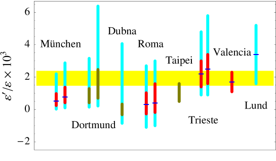
Figure 2.  : Summary of theoretical estimates for $\varepsilon^{\prime}/\varepsilon$ . The dark (light) range corresponds to Gaussian (flat) scanning of the uncertainties. The gray horisontal band is the average experimental result.

• München[5]: The $\Delta I=1/2$ rule is fitted (at $\mu=m_{c}$). Unfortunately, this does not give (enough) information about the matrix elements of $Q_{6,8}$. These are varied around their leading $1/N_{c}$ values.

• Roma[21]: This is the only first principle estimate. Some matrix elements have been calculated, but unfortunately not that of $Q_{6}$, which is varied by 100% around its VSA value. Also the “penguin contractions” of $Q_{1,2}$ needed to explain the $\Delta I=1/2$ rule are difficult to obtain.

• Dortmund [22]: The quark operators are matched (between 600 and 900 MeV) directly to their corresponding chiral loops with a quadratic cut-off, carefully identified with the renormalization scale.

• Dubna[23]: Uses extended Nambu Jona-Lasinio (ENJL) models and chiral loops regularized by the heat kernel. It is found that chiral loops to $O(p^{6})$ have sizeable absorptive parts bur rather small real parts.

• Taipei[24]: Uses “generalized factorization” where scheme dependence is absorbed in effective Wilson coefficients. Non-factorizable contribtions in (16,27) are represented by a phenomenological parameter.

• Valencia[25]: Special attention is put on FSI effects. A dispersion relation is used, and the analysis confirms the importance of chiral loops.

• Lund[26]: A EJNL framework including axial and vector resonances. Care is taken to match LD and SD calculations. A sizeable enhancement of the $Q_{6}$ contribution is found, which predicts $\varepsilon^{\prime}/\varepsilon$ on the high side.

Also, an estimate using a linear sigma model [27] shows enhancement of the $Q_{6}$ matrix element, but its hard to explain the $\Delta I=1/2$ rule and $\varepsilon^{\prime}/\varepsilon$ at the same time within this approach.

4 Conclusions

All groups have to a certain extent used assumptions and models. Still, most estimates are roughly in the right ballpark, as seen from Fig. 2. Given the hadronic uncertainties, it will be hard to disentangle new physics from the SM predictions.

*   *   *

I thank the organizers of this meeting, and my collaborators S. Bertolini and M. Fabbrichesi.

References

- [1] Winstein,B and Wolfenstein, L. (1993) Rev. Mod. Phys. 65, 1113-1148.
-
[2]
E. de Rafael, E. (1994) in CP Violation and the Limits of the
Standard Model,
Benjamin/Cummings Publ. -
[3]
Buchalla, G., Buras, A.J. and Lautenbacher, M.E. (1996)
Rev. Mod. Phys. 68, 1125-1144. -
[4]
Bertolini, S., Eeg, J.O., Fabbrichesi, M.
(2000) Rev. Mod. Phys. 72, 65-93;
e-Print Archive: hep-ph/9802405. - [5] Bosch, S. et al. (1999) Nucl. Phys. B565 3-37.
-
[6]
Bertolini, S., Eeg, J.O., Fabbrichesi, M. (2000),
e-Print Archive: hep-ph/0002234;
Bertolini, S. (2000), hep-ph/0007137; Fabbrichesi, M. (2000), hep-ph/0009321. -
[7]
Se for example: Pich, A. (1998) in
Probing the Standard Model of Particle Interactions,
Les Houches Summer School, France, 28 Jul - 5 Sep 1997;
e-Print Archive: hep-ph/9806303. - [8] Cirigliano, V., Donoghue, J.F. and Golowich, E. (2000) hep-ph/0007196.
- [9] Buras, A.J., Jamin, M. and Lautenbacher, M.E. (1993) Nucl. Phys. B400, 75-102.
-
[10]
Ciuchini, M.,Franco, E., Martinelli, G. and Reina, L. (1994)
Nucl. Phys. B415, 403-462. - [11] Bertolini, S., Eeg, J.O., Fabbrichesi, M. (1995) Nucl. Phys. B449, 197-225.
- [12] Bergan, A.E. and Eeg, J.O. (1997), Phys. Lett. B390, 420-426.
-
[13]
Penin, A.A. and Pivovarov, A.A. (1994) Phys.Rev D49, 265-268;
Melsom, J. (1997) Z. Phys. C75, 471-476. - [14] See refs. [11,12,15-18] and references therein.
- [15] Pich, A. and de Rafael, E. (1991) Nucl. Phys. B358, 311-382.
-
[16]
Antonelli, V., Bertolini, S., Eeg, J.O., Fabbrichesi, M. and Lashin, E.I.
(1996)
Nucl. Phys. B469, 143-180. -
[17]
Bertolini, S., Eeg, J.O., Fabbrichesi, M. and Lashin, E.I. (1998)
Nucl. Phys. B514, 63-92. -
[18]
Bertolini, S., Eeg, J.O., Fabbrichesi, M. and Lashin, E.I. (1998)
Nucl. Phys. B514, 93-112. - [19] Alavi-Harati, A. et al (1999) Phys. Rev. Lett. 83, 22-27.
- [20] Fanti, V. et al. (1999) Phys. Lett. B465, 335-348.
- [21] Ciuchini, M. et al. (2000) Nucl. Phys. B573, 201-222.
- [22] Hambye, T. et al. (2000) Nucl. Phys. B564, 391-429.
- [23] Be’lkov, A.A. et al hep-ph/9907335.
- [24] Cheng, H.-Y., (1999) hep-ph/9911202.
- [25] Pallante, E. and Pich, A. (2000) Phys. Rev. Lett 84, 2568-2571.
- [26] Bijnens,J. and Prades, J. (2000) hep-ph/0005189.
- [27] Keum, Y.Y., Nierste, U. and Sanda, A. (1999) Phys. Lett. B457, 157-162.