Abstract

It is argued that the gluon density introduced by A.Mueller [5] in relation to the saturation phenomenon is different from the standardly defined one, which turned out to have a soliton-like form in the numerical calculations. It is shown that A.Mueller’s densities obtained from the latter possess the same saturation properties as originally predicted.

1 Introduction

The idea of parton saturation in large nuclei has recently obtained much attention [1-5]. In particular A.Mueller has discussed in [5] the behaviour of the quark and gluon densities for different values of momenta in a large nucleus. In his treatment the interaction of the probing current and the nucleons of the target was taken in the Glauber form, with the parton-nucleon amplitude taken in the two-gluon exchange approximation. The evolution of the gluonic distribution in $x$ has not been studied. The result of these study is that the behaviour of both the quark and gluonic distribution in the momentum $l$ is determined by a cerain critical ”saturation momentum” defined as

$$Q^{2}_{s}=c\frac{8\pi^{2}\alpha_{s}N_{c}}{N_{c}^{2}-1}AT(b),$$ (1)

with $T(b)$ the standard nuclear profile function and $c$ essentially a constant. At high momenta $l^{2}>>Q_{s}^{2}$ the distributions retain their perturbative form

$${d\big{(}xq(x,Q^{2})\big{)}\over d^{2}bd^{2}\ell}={N_{c}\over 6\pi^{4}}\ {Q_{s}^{2}\over\ell^{2}}\$$ (2)

and

$${d\big{(}xG(x,Q^{2})\big{)}\over d^{2}bd^{2}\ell}={N_{c}^{2}-1\over 4\pi^{4}}{Q_{s}^{2}\over\ell^{2}}\ln\frac{1}{x}\ \ \ \ {\rm for}\ \ \ell^{2}>>Q_{s}^{2}.$$ (3)

for the quark and gluon distributions respectively. However as the momentum $l$ diminishes both distributions do not infinitely grow (as would follow from (2) and (3)) but saturate at a certain finite value. In fact at $l^{2}<<Q_{s}^{2}$ A.Mueller found

$${d\big{(}xq(x,Q^{2})\big{)}\over d^{2}bd^{2}\ell}={N_{c}\over 2\pi^{4}}$$ (4)

and

$${d\big{(}xG(x,Q^{2})\big{)}\over d^{2}bd^{2}\ell}\approx{N_{c}^{2}-1\over 4\pi^{4}}\ln\frac{1}{x}\ \ \ {\rm for}\ \ \ell^{2}<<Q_{s}^{2}.$$ (5)

Independently of the saturation problem, in the last year the interaction of a probe with a large nucleus at small $x$ was studied in the perturbative QCD with reggeized gluons. It reduces to summing fan diagrams constructed of BFKL pomerons with a splitting triple Pomeron vertex [6-9]. In [9] the resulting equation was solved numerically, which enabled us to calculate the corresponding gluon distribution. Its features turned out to be somewhat different from what has been found by A.Mueller. Although at large $l$ the gluonic distribution indeed falls down similarly to the perturbative result and to what has been found in [5], it also falls down to zero at small $l^{2}$. The form of the found gluonic distribution as a function of $\log\ l$ is close to a Gaussian with a constant height and a center moving with a constant velocity to higher $l$ as the rapidity $y$ increases . Thus in the $(\log\ l,y)$ space the gluonic density turns out to be a soliton wave.

This unexpected behaviour of the gluonic density caused some mistrust due to the seemingly sound base of the analytic derivation of A.Mueller and a purely numerical character of the calculations in [9]. Here we intend to study the reasons for the difference of these results.

One might think that this difference is due to a complicated gluonic interaction introduced in the approach pursued in our numerical calculation and absent in the picture of A.Mueller. However the answer seems to be much simpler: the gluonic densities studied in both papers are in fact different quantities. While the gluonic density numerically calculated in [9] is more or less standard, the one introduced by A.Mueller is a new quantity. We show that for this latter density our numerical results indeed lead to the same saturation as in [5]. Moreover, A.Mueller’s quark density found from our solitonic gluon density also exhibits the same saturation properties as found in [5].

Besides showing that there is no contradiction between [5] and [9] at all, this confirms that the gluonic interaction at small $x$ and the resulting very sophisticated dynamical picture do not actually influence the saturation properties of A.Mueller’s densities, as conjectured in [5].

Of course there remains a question, which is the “correct” parton density. As we argue in the last section, we beleive that the densities introduced by A.Mueller do not in general describe partonic distributions in the target.

2 Gluonic distributions: standard and of A.Mueller

We begin with the definition of the gluonic density adopted in our numerical calculations, which we call ”standard”. It can be taken from the standard expression for the structure function of the nucleus in its terms (see e.g [10 ])

$$F_{2}(x,Q^{2})=\frac{4\alpha_{s}Q^{2}}{\pi^{2}N_{c}e^{2}}\int d^{2}bd^{2}r[\rho_{T}(r)+\rho_{L}(r)]f(x,r,b),$$ (6)

where $\rho_{T,L}$ are the transverse and longitudinal colour densities created by the incoming photon and $f$ is expressed via the double density of gluons in momentum and impact parameter:

$$f(x,r,b)=\int\frac{d^{2}k}{(2\pi)^{2}k^{2}}\frac{d\big{(}xG(x,k^{2},b)\big{)}}{d^{2}bdk^{2}}\left(1-e^{-ikr}\right)\left(1-e^{ikr}\right).$$ (7)

In [9] it was found that, up to a factor, fuction $f$ coincides with a sum of BFKL fan diagrams $\Phi$

$$f(x,r,b)=\frac{N_{c}}{2\pi^{3}\alpha_{s}}\Phi(x,r,b).$$ (8)

Taking a Fourier transform of (7) and neglecting the term proportional to $\delta^{2}(k)$ we obtained

$$\frac{d\big{(}xG(x,k^{2},b)\big{)}}{d^{2}bdk^{2}}=\frac{N_{c}}{2\pi^{2}\alpha_{s}}k^{2}\nabla_{k}^{2}\phi(x,k,b)\equiv\frac{N_{c}}{2\pi^{2}\alpha_{s}}h(x,k,b),$$ (9)

where in the coordinate space

$$\phi(x,r,b)=\frac{\Phi(x,r,b)}{2\pi r^{2}}.$$ (10)

Function $\phi$ was found in [9] by numerical solution of the BFKL fan diagram equation. Applying $k^{2}\nabla_{k}^{2}$ to it we found the gluon density. As mentioned in the Introduction, at any given rapidity the density turned out to have the same, roughly Gaussian, shape in variable $\xi=\ln k$, centered at the point $\xi=\xi_{0}(y)$, which moves to the right with a nearly constant velocity. Approximately the distribution can be described by

$$h(k)=h_{0}e^{-a(\xi-\xi_{0}(y))^{2}},$$ (11)

where $h_{0}$ and $a$ are practically independent of $y$ and $\xi_{0}(y)$ linearly grows with it:

$$h_{0}\simeq 0.3,\ \ \xi_{0}(y)=c+0.222\ln A+2.23\frac{\alpha_{s}N_{c}}{\pi}y.$$ (12)

It can be shown that it is normalized according to

$$\int_{0}^{\infty}\frac{dk}{k}h(y,k,b)=1,$$ (13)

which condition relates $a$ and $h_{0}$. The starting position of the center $c$ depends on the initial distribution at small rapidities.

Evidently at a given value of $k$ the density always remains limited, irrespective of the form of the initial distribution (and on the atomic number $A$, in particular). In this sense we have saturation as discussed in [1-5]. However with the growth of $y$ the strongly peaked density moves away toward higher values of $k$ so that the density at a fixed point tends to zero at high values of rapidity. We thus find “supersaturation”: with $y\rightarrow\infty$ the gluon density at an arbitrary finite momentum tends to zero.

Now we pass to the gluon density introduced by A.Mueller. He related it to a particular process, analogous to the $\gamma^{*}$-target scattering, in which the electromagnetic current is changed to a “gluonic” current

$$j(x)=-{1\over 4}F_{\mu\nu}^{i}F_{\mu\nu}^{i}.$$ (14)

This current generates a colourless pair of gluons, which according to [5] interact with the target very much in the same way as a $q\bar{q}$ pair generated by the electromagnetic current (see Fig. 1, diagrams $b$ and $c$). The gluon density is then defined as a contribution to the cross-section from a given value of the transverse momentum $l$ of the struck gluon on the left part of the diagrams.

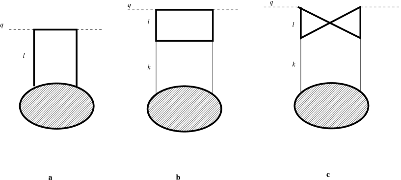
Figure 1: Interaction of a probe with the target. Thick lines show partons (gluons or quarks) directly coupled to the probe. Thin lines show exchanged gluons.

For the case when the target is just a nucleon, in the limit $Q^{2}\rightarrow\infty$ and in the single gluon exchange exchange approximation, A.Mueller found for his density, which we denote $xG_{M}(x,Q^{2},l^{2})$ (it generally depends on two different momenta):

$${d\big{(}xG_{M}(x,Q^{2},\ell^{2})\big{)}\over d^{2}\ell}={\alpha N_{c}\over 2\pi^{5}}\ \int_{x\ell^{2}/Q^{2}}^{\ell^{2}/Q^{2}}{dz\over z}\ {d^{2}r_{1}d^{2}r_{2}\over r_{1}^{2}r_{2}^{2}}\ e^{-i{\ell}\cdot(r_{1}-r_{2})}({2(r_{1}r_{2})^{2}\over r_{1}^{2}r_{2}^{2}}-1)$$

$$\cdot(1+e^{-i{}{k}\cdot({}r_{1}-{}r_{2})}-e^{-i{}{k}\cdot{}r_{1}}-e^{i{}{k}\cdot{}r_{2}}){d^{2}k\over k^{2}}\ {d\big{(}xG(x,k^{2})\big{)}\over dk^{2}}.$$ (15)

On the right-hand side there appeared $xG(x,k^{2})$, which is just the standard gluonic density. In the approximations made in deriving (15) it does not depend on $x$, nor the whole expression depends on $Q^{2}$. As a result, the gluon density defined by (15) also depends on only one momentum squared $\ell^{2}$ and superficially looks similar to the standard gluon density. But in fact it is a different quantity (factor $\alpha_{s}$ in front of (15) is already sufficient to see it). Its physical meaning has been explained before: it is a probability to find one of the struck gluons (the left one in the Fig. 1) with momentum $\ell$. Later we shall discuss to what extent this quantity probes the gluon distribution in the nucleon.

We see that once the standard $xG$ is known, the density $xG_{M}$ can be found directly from Eq. (15). This exersize is done in the next section.

3 The soliton density and saturation

The first thing to do is to generalize $xG_{M}$ to the nucleus target. Having in mind the fan diagram picture for the interaction of a probe with the nucleus, on the one hand, and the scattering process considered by A.Mueller to define his density, on the other, all we have to do is to change the standard density $xG$ on the right- hand side of Eq. (15) to the same quantity for the nucleus:

$${d\big{(}xG_{M}(x,Q^{2},\ell^{2},b)\big{)}\over{d^{2}bd^{2}\ell}}={\alpha N_{c}\over 2\pi^{5}}\ \int_{x\ell^{2}/Q^{2}}^{\ell^{2}/Q^{2}}{dz\over z}\ {d^{2}r_{1}d^{2}r_{2}\over r_{1}^{2}r_{2}^{2}}\ e^{-i\ell\cdot(r_{1}-r_{2})}({2(r_{1}r_{2})^{2}\over r_{1}^{2}r_{2}^{2}}-1)$$

$$\cdot(1+e^{-ik\cdot(r_{1}-r_{2})}-e^{-i{k}\cdot r_{1}}-e^{i{k}\cdot r_{2}}){d^{2}k\over k^{2}}\ {d\big{(}xG\big{)}\over{d^{2}bdk^{2}}}.$$ (16)

Here we suppresed all evident arguments in $G$ on the right-hand side. This will be also often done in the following when the arguments are obvious.

We want to calculate this expression taking for $d(xG)/d^{2}bdk^{2}$ the solitonic gluon distribution in a nucleus obtained by our numerical studies. In principle this can be done rigorously, by numerical integration. However, since we are interested in the qualitative features of the saturation behaviour, we shall adopt here a simpler approach. We shall use the fact that at large rapidities the solitonic distribution is strongly peaked at the momena determined by

$$k_{0}=e^{\xi_{0}}\sim A^{2/9}\exp\left(2.23\frac{N_{c}\alpha_{s}}{\pi}y\right)$$ (17)

(which are very high already at reasonable $y$ for not very small $\alpha_{s}$). This momentum will play the role of Mueller’s saturation momentum $Q_{s}$. Assuming that $k_{0}^{2}<<Q^{2}$ one can take all the integrand out of the integral over $k$ at point $k=k_{0}$ except for the density factor. The latter, integrated over $k^{2}$ gives $N_{c}/(2\alpha_{s}\pi^{2})$ according to (9) and the normalization condition (13). So we are left with the expression

$${d\big{(}xG_{M}\big{)}\over{d^{2}bd^{2}\ell}}={N_{c}^{2}\over 4\pi^{7}}\ln\frac{1}{x}\int d\phi\ {d^{2}r_{1}d^{2}r_{2}\over r_{1}^{2}r_{2}^{2}}\ e^{-i\ell\cdot(r_{1}-r_{2})}({2(r_{1}r_{2})^{2}\over r_{1}^{2}r_{2}^{2}}-1)$$

$$\cdot(1+e^{-i{}{k}\cdot({}r_{1}-{}r_{2})}-e^{-i{}{k}\cdot{}r_{1}}-e^{i{}{k},\cdot{}r_{2}})$$ (18)

where one should take $k=k_{0}n$ with a two dimensional unit vector $n$.

Calculation of the integrals over $r_{1}$ and $r_{2}$ is simplified by using the identity

$$\frac{1}{r_{1}^{2}r_{2}^{2}}\left(\frac{2(r_{1}r_{2})^{2}}{r_{1}^{2}r_{2}^{2}}-1\right)=\frac{1}{2}(\nabla_{1}\nabla_{2})^{2}\ln r_{1}\ln r_{2}.$$ (19)

One obtains

$${d\big{(}xG_{M}\big{)}\over{d^{2}bd^{2}\ell}}={N_{c}^{2}\over 8\pi^{7}}\ln\frac{1}{x}\int d\phi\Big{[}X(l,l)+X(l+k,l+k)-2X(l+k,l)\Big{]},$$ (20)

where

$$X(l_{1},l_{2})=\int d^{2}r_{1}d^{2}r_{2}e^{il_{1}r_{1}+il_{2}r_{2}}(\nabla_{1}\nabla_{2})^{2}\ln r_{1}\ln r_{2}=4\pi^{2}\frac{(l_{1}l_{2})^{2}}{l_{1}^{2}l_{2}^{2}}.$$ (21)

This leads to

$${d\big{(}xG_{M}\big{)}\over{d^{2}bd^{2}\ell}}={N_{c}^{2}\over\pi^{5}}\ \ln\frac{1}{x}\int d\phi\frac{l^{2}k_{0}^{2}-(lk)^{2}}{l^{2}(l+k)^{2}}.$$ (22)

Let us consider the two limiting cases studied in [5]. If $l>>k_{0}$ then one finds from (22)

$${d(xG_{M})\over{d^{2}bd^{2}\ell}}={N_{c}^{2}\over\pi^{4}}\ \frac{k_{0}^{2}}{l^{2}}\ln\frac{1}{x}.$$ (23)

In the opposite case $l^{2}<<k_{0}^{2}$ we find

$${d(xG_{M})\over{d^{2}bd^{2}\ell}}={N_{c}^{2}\over\pi^{4}}\ \ln\frac{1}{x}$$ (24)

This behaviour is identical with (3) and (5) (for $N_{c}>>1$ and except for factor 4 in (24)).

So Mueller’s density indeed saturates to a finite value at small $l^{2}$ irrespective of the dynamical picture. The standard density however behaves very differently and for a heavy nucleus goes to zero at any fixed value of $l$ as the rapidity gets large enough.

4 The quark density from the soliton gluonic density

Following [5] and similarly to the gluon case, one may introduce a quark distribution depending on two momenta squared $xq_{M}(x,Q^{2},\ell^{2})$, as a contribution from the left struck quark to the cross-section corresponding to diagrams $b$ and $c$ in Fig. 1. In the two-gluon exchange approximation for the interaction, this quantity again results independent of $Q^{2}$ at high virtualities. We postpone discussion of the relation of this limiting distribution in $\ell$, $xq_{M}(x,\ell^{2})$ to the standard quark density as a function of $Q^{2}$, $xq(x,Q^{2})$, until the last section. Here we shall consider the properties of $xq_{M}(x,\ell^{2})$ which follow from the found standard gluon distribution in a large nucleus.

The definition of $xq_{M}(x,Q^{2},\ell^{2})$ is very similar to that of (15). For a single nucleon as a target A.Mueller found:

$${d\big{(}xq(x,Q^{2},\ell^{2})\big{)}\over d^{2}\ell}={\alpha Q^{2}\over 4\pi^{3}}\int_{0}^{1}dz[z^{2}+(1-z)^{2}]\left(\frac{\ell^{2}}{\ell^{2}+\epsilon^{2}}-{(\ell,\ell+k)\over{(\ell^{2}+\epsilon^{2})[(\ell+k)^{2}+\epsilon^{2}]}}\right){d^{2}k\over k^{2}}\ {dxG\over dk^{2}},$$ (25)

where

$$\epsilon^{2}=Q^{2}z(1-z).$$ (26)

As one observes, the quark density $xq_{M}$ is again defined via the standard gluon density.

For the nucleus target, as explained before, all we have to do is to take the corresponing nuclear density on the right-hand side of (25):

$${d\big{(}xq_{M}\big{)}\over d^{2}bd^{2}\ell}={\alpha Q^{2}\over 4\pi^{3}}\int_{0}^{1}dz[z^{2}+(1-z)^{2}]\left(\frac{\ell^{2}}{\ell^{2}+\epsilon^{2}}-{(\ell,\ell+k)\over{(\ell^{2}+\epsilon^{2})[(\ell+k)^{2}+\epsilon^{2}]}}\right){d^{2}k\over k^{2}}\ {dxG\over d^{2}bdk^{2}}.$$ (27)

At high $Q^{2}$ evidently only small $z$ or $1-z$ contribute. Then integrating over $\epsilon^{2}\simeq Q^{2}z$ we find

$${d\big{(}xq_{M}\big{)}\over d^{2}bd^{2}\ell}={\alpha\over 2\pi^{3}}\int{d^{2}k\over k^{2}}\ {dxG\over d^{2}bdk^{2}}\left(1-\frac{(l,l+k)}{(l+k)^{2}-l^{2}}\ln\frac{(l+k)^{2}}{l^{2}}\right).$$ (28)

Let us take for $xG$ the soliton-like gluon density found in [9]. As before we take all smooth functions out of the integral over $k$ and afterwards integrate over $k$ using (13). We obtain

$${d\big{(}xq_{M}\big{)}\over{d^{2}bd^{2}\ell}}={N_{c}\over 4\pi^{5}}\int d\phi\Big{[}1-\frac{(l,l+k)}{(l+k)^{2}-l^{2}}\ln\frac{(l+k)^{2}}{l^{2}}\Big{]}$$ (29)

where $k=k_{0}n$ as in the preceding section.

Again we shall concentrate on the two limiting cases. If $l>>k_{0}$ using

$$\frac{1}{(l+k)^{2}-l^{2}}\ln\frac{(l+k)^{2}}{l^{2}}\simeq\frac{1}{l^{2}}\Big{(}1-\frac{1}{2}\frac{2(lk)+k^{2}}{l^{2}}+\frac{4}{3}\frac{(lk)^{2}}{l^{4}}\Big{)}$$

and integrating over the angle $\phi$ we get

$${d\big{(}xq_{M}\big{)}\over{d^{2}bd^{2}\ell}}={N_{c}\over 6\pi^{4}}\frac{k_{0}^{2}}{l^{2}}.$$ (30)

In the opposite case $l^{2}<<k_{0}$ the second term in the bracket of (29) does not contribute and we get

$${d\big{(}xq_{M}\big{)}\over{d^{2}bd^{2}\ell}}={N_{c}\over 2\pi^{4}}.$$ (31)

This behaviour exactly coincides with A.Mueller results (2) and (4).

5 Discussion

As we have seen, there are in fact two different gluon densities, which exhibit different behaviour as functions of momenta. The standard one defined via Eq (7) has a soliton-like behaviour and vanishes at any given $\ell$ as $y\rightarrow\infty$. The other, defined in [5], saturates at small momenta to a finite value, which turns out to be universal in the sense that it does not depend on the complexity of the interaction mechanism. Which of the two densities is the “correct” one?

The definition of the standard gluon density via Eq. (7) seems to us perfectly adequate. Its validity is clear from the inspection of the diagrams $b$ and $c$ of the Fig. 1 corresponding to (7). The lower gluonic blob, to which the quark loop is coupled, has to be integrated over the “-” component of the 4-momentum k (in a system, in which the target has momentum with a large “+” component). Evidently ihe blob then represents just the gluonic density at a given “time” $x_{+}$.

Interpretation of Mueller’s density, in contrast, is not so obvious. First, in the presence of the interference diagram $c$ of Fig. 1, one may hardly say that the contribution from the left struck gluon to the cross-section probes the gluon distribution in the target. In the interference diagram the right struck gluon has a different transverse momentum $\ell+k$, so that the interpretation of the whole contribution as a gluon density is doubtful. Then it is not clear why the lowest order diagram Fig. 1$a$ has not been included. Finally, in the BFKL kinematics the virtual gluons tend to reggeize. One then expects that the interference digram can be neglected and diagram Fig. 1$b$ will be absorbed into $a$ to form a BFKL pomeron coupled to the target. So in the end one will find only the diagram Fig. 1$a$, which leads to the standard gluon density as defined through Eq. (7).

The same doubts refer to the quark density in the definition of A.Mueller. Again, so long as one cannot neglect the interference diagram, the interpretation of the contribution to the cross-section from the left struck quark with a given momentum as a quark density of the target does not seem possible. True, in the DGLAP kinematics, with finite $x$ , the interference diagram can indeed be neglected, substituted by the requirement that $\ell^{2}<<Q^{2}$. However then one has the transverse momentum ordering and the density found from Eq. (25) would be trivial (see [5], Eq. (14)). In the BFKL regime, at small $x$, the virtual quarks also tend to reggeize and the contribution from digram Fig. 1$c$ hopefully becomes neglegible as compared to $a$ and $b$, which actually become identical. Then the interpretation of (25) as the quark density may aquire sense. However to calculate it one should couple the found gluonic distribution to a reggeized quark. We leave this problem for future studies.

6 References

1. L.V. Gribov, E.M. Levin and M.G. Ryskin, Phys.Rep.100 (1983)1.

2. A.H. Mueller, Nucl.Phys.B335 (1990) 115.

3. J.Jalilian-Marian, A. Kovner, L.McLerran and H. Weigert, Phys.Rev.D55 (1997) 5414.

4. Yu. V. Kovchegov and A.H. Mueller, Nucl.Phys.B529 (1998) 451.

5. A.H.Mueller, hep-ph/9904404

6. I.Balitsky, hep-ph/9706411; Nucl. Phys. B463 (1996) 99.

7. Yu. Kovchegov, Phys. Rev D60 (1999) 034008;
preprint CERN-TH/99-166 (hep-ph/9905214).

8.E.Levin and K.Tuchin, preprint DESY 99-108, TAUP 2592-99 (hep-ph/9908317).

9. M.A.Braun, Eur.Phys. J. C16 (2000) 337-348.

10. M.A.Braun, Eur. Phys. J C6 (1999) 343.