1 Introduction

Quark and gluon fields are the basic objects of Quantum Chromodynamics (QCD), the theory of strong interactions. On the other hand, the objects observable in experiment are hadrons, which are built up from quarks and gluons. There is still no analytical description of the mechanism of confinement which relates hadron properties to the quark and gluon degrees of freedom. In hard scattering processes, instead, we parameterise the non-perturbative information in terms of hadronic matrix elements of quark and gluon field operators. Universality of the matrix elements assures that once they have been measured in a hard process, the results can be plugged into the calculation of observables for other hard processes.

In the description of inclusive and exclusive hard processes the hadronic matrix elements of quark and gluon fields generally are of two distinct types:

• In inclusive hard processes the hadron state expectation values, i.e., diagonal matrix elements, of bi-local combinations of field operators at a light-like distance are conveniently expressed in terms of parton distribution functions (PDFs) [1]. At leading order in a twist expansion the PDFs acquire a simple intuitive interpretation in the context of light-cone (LC) quantisation, provided a light-cone gauge, for instance $A^{+}=0$, is used. In that case, the PDFs give the probability to find a parton inside a hadron, carrying the plus-component fraction $x$ of the hadron’s momentum $p$. Projections on definite helicity or transverse spin eigenstates of the partons reveal information on their preferences to be aligned or anti-aligned relative to the spin of the parent hadron. The polarised quark PDFs, like the helicity distribution $\Delta q(x)$ or the transverse spin distribution $\delta q(x)$, thus have an interpretation as differences of probabilities.

• The other type of hadronic matrix elements of quark and gluon fields is involved in the description of hadron form factors at large momentum transfers. They are defined from matrix elements of local combinations of quark field operators. In contrast to the above mentioned matrix elements of the inclusive processes, the matrix elements involved in the definition of form factors are non-diagonal in initial and final state, which are characterised by different momenta.

The interest in the connection between hard inclusive and exclusive reactions has recently been renewed in the context of the so-called skewed parton distributions (SPDs) [2, 3, 4] which have been shown to play a decisive role in the understanding of deeply virtual exclusive reactions, Compton scattering [4, 5] and electroproduction of mesons [6]. The SPDs, defined as non-diagonal hadronic matrix elements of bi-local products of quark and gluon field operators, are functions of the momentum fraction variable $\bar{x}$, the skewedness parameter $\xi$, and the squared momentum transfer $t$ (see Sect. 2 for definitions). They represent generalisations of the two types of hadronic matrix elements mentioned above and are, in so far, hybrid objects which combine properties of ordinary PDFs and of form factors. In fact, the close connection of these quantities becomes manifest in reduction formulas: PDFs are the forward limits of the SPDs, while form factors are moments of them.

In a recent publication [7] we have obtained a representation of quark SPDs in the regions $\xi<|\bar{x}|<1$ in terms of light-cone wave function (LCWF) overlaps. This representation can be viewed as a generalisation of the famous Drell-Yan formula [8] for electromagnetic form factors. It also includes the LCWF representation of the PDFs [9] as a limiting case. The purpose of the present article is to present the derivation of the overlap representation for SPDs in detail within the framework of the light-cone (LC) quantisation. We will generalise our previous result [7] to the entire kinematical region, $-1<\bar{x}<1$, and extend it to the gluonic sector.

The paper is organised as follows: In Sect. 2 we recall a few basic facts of LC quantisation, discuss the Fock state decomposition of hadronic states, and introduce the relevant kinematical definitions. The derivation of the overlap representation for the unpolarised quark SPDs is presented in some detail in Sect. 3. The case of polarised quark SPDs and the extension to the case of gluons is discussed in Sect. 4. Sect. 5 is devoted to the discussion of general properties of the overlap representation, and Sect. 6 to phenomenological applications. We conclude the article with a summary (Sect. 7). In an appendix we will present some useful formulas in order to facilitate the comparison with other conventions in the definition of SPDs.

2 Fock state decomposition

In this Section, after giving some necessary definitions for field operators and parton states, we discuss the Fock state decomposition of a hadronic state, a crucial step towards an overlap representation of SPDs. We will use the component notation $z^{\mu}=\left[z^{+},z^{-},{\bf z}_{\perp}\right]$ for any four-vector $z$ with the LC components $z^{\pm}=(z^{0}\pm z^{3})/\sqrt{2}$ and the transverse part ${\bf z}_{\perp}=(z^{1},z^{2})$. We will work in the framework of LC quantisation in the $A^{+}=0$ gauge. At given light-cone time, say $z^{+}=0$, the independent dynamical fields are the so-called “good” LC components of the fields, namely $\phi_{q}^{\,c}\equiv P_{+}\psi_{q}^{\,c}$ for quarks of flavour $q$ and colour $c$ (where the projectors acting on the Dirac field $\psi_{q}^{\,c}$ are defined by $P_{\pm}=\frac{1}{2}\gamma^{\mp}\gamma^{\pm}$) and the transverse components of the gluon potential $A_{\alpha}^{\,c}$ (where $\alpha\in\{1,2\}$ is a transverse index and $c$ again denotes colour). The independent dynamical fields have Fourier expansions in momentum space (see e.g. [9], Appendix II)

$$\phi_{q}^{\,c}(z^{-},{\bf z}_{\perp}) = \int\frac{{\rm d}k^{+}\,{\rm d}^{2}{\bf k}_{\perp}}{k^{+}\,16\pi^{3}}\,\Theta(k^{+})\;\sum_{\mu}\;$$ (1)

$$\bigg{\{}\phantom{{}+{}}b_{q}(w)\;u_{+}(w)\;\exp\left({}-i\,k^{+}z^{-}+i\,{\bf k}_{\perp}\cdot{\bf z}_{\perp})\right)$$

$$\phantom{\bigg{\{}}{{}+{}}d_{q}^{\,\dagger}(w)\,v_{+}(w)\;\exp\left({}+i\,k^{+}z^{-}-i\,{\bf k}_{\perp}\cdot{\bf z}_{\perp})\right)\bigg{\}}$$

for the free quark field, and ($\alpha\in\{1,2\}$)

$$A_{\alpha}^{\,c}(z^{-},{\bf z}_{\perp}) = \int\frac{{\rm d}k^{+}\,{\rm d}^{2}{\bf k}_{\perp}}{k^{+}\,16\pi^{3}}\,\Theta(k^{+})\;\sum_{\mu}$$ (2)

$$\bigg{\{}\phantom{{}+{}}a^{\phantom{.}}(w)\;\epsilon_{\alpha}(w)\;\exp\left({}-i\,k^{+}z^{-}+i\,{\bf k}_{\perp}\cdot{\bf z}_{\perp}\right)$$

$$\phantom{\bigg{\{}}{{}+{}}a^{\,\dagger}(w)\,\epsilon^{*}_{\alpha}(w)\;\exp\left({}+i\,k^{+}z^{-}-i\,{\bf k}_{\perp}\cdot{\bf z}_{\perp}\right)\bigg{\}}\>.$$

for the free gluon field, where $\Theta(k^{+})$ denotes the usual step function. We use a collective notation for the dependence on the plus and transverse parton momentum components, the helicity, and the colour in the form

$$w=(k^{+},{\bf k}_{\perp},\mu,c)\>.$$ (3)

The operators $b$ and $d^{\dagger}$ are the annihilator of the “good” component of the quark fields and the creator of the “good” component of the antifields, respectively, and $u_{+}(w)\equiv P_{+}\,u(w)$ and $v_{+}(w)\equiv P_{+}\,v(w)$ are the projections of the usual quark and antiquark spinors. $a$ and $a^{\dagger}$ are the annihilation and creation operators for transverse gluons, and $\epsilon_{\alpha}(w)$ is a transverse component of the gluon polarisation vector. The operators fulfil the anticommutation relations

$$\left\{b_{q^{\prime}}^{\phantom{.}}(w^{\prime}),b_{q}^{\,\dagger}(w)\right\} = \left\{d_{q^{\prime}}^{\phantom{.}}(w^{\prime}),d_{q}^{\,\dagger}(w)\right\}$$ (4)

$$= 16\pi^{3}\;k^{+}\;\delta(k^{\prime\,+}-k^{+})\;\delta^{(2)}\left({\bf k}^{\prime}_{\perp}-{\bf k}_{\perp}\right)\;\delta_{q^{\prime}q}\;\delta_{\mu^{\prime}\mu}\;\delta_{c^{\prime}c}\>,$$

and the gluon operators $a$ and $a^{\dagger}$ satisfy the commutation relation

$$\left[a^{\phantom{.}}(w^{\prime}),a^{\,\dagger}(w)\right]=16\pi^{3}\;k^{+}\;\delta(k^{\prime\,+}-k^{+})\;\delta^{(2)}\left({\bf k}^{\prime}_{\perp}-{\bf k}_{\perp}\right)\;\delta_{\mu^{\prime}\mu}\;\delta_{c^{\prime}c}\>.$$ (5)

Key ingredient in our derivation of the overlap representation is the Fock state decomposition [9], i.e., the replacement of a hadron state by a superposition of partonic Fock states containing free quanta of the “good” LC components of (anti)quark and gluon fields. Single-parton, quark, antiquark or gluon, momentum eigenstates are created by $b^{\dagger}$, $d^{\dagger}$ and $a^{\dagger}$ acting on the perturbative vacuum,

$$|q;w\rangle = b_{q}^{\dagger}(w)\,|0\rangle\>,$$

$$|\bar{q};w\rangle = d_{q}^{\dagger}(w)\,|0\rangle\>,$$

$$|g;w\rangle = a^{\dagger}(w)\,|0\rangle\>,$$ (6)

and the (anti)commutation relations (4) and (5) translate into the normalisation of these states,

$$\langle s^{\prime};w^{\prime}|s;w\rangle=16\pi^{3}\,k^{+}\,\delta(k^{\prime\,+}-k^{+})\,\delta^{(2)}\left({\bf k}^{\prime}_{\perp}-{\bf k}^{\phantom{.}}_{\perp}\right)\delta_{s^{\prime}s}\;\;\delta_{\mu^{\prime}\mu}\;\delta_{c^{\prime}c}$$ (7)

for partons $s$, $s^{\prime}$ of any kind. A hadronic state characterised by the momentum $p$ and helicity $\lambda$ is written as

$$\left|H;p,\lambda\right\rangle=\sum_{N,\beta}\int[{\rm d}x]_{N}[{\rm d}^{2}{\bf k}_{\perp}]_{N}\;\Psi_{N,\beta}^{\lambda}(r)\;\left|N,\beta;k_{1},\ldots,k_{N}\right\rangle\>,$$ (8)

where $\Psi_{N,\beta}^{\lambda}(r)$ is the momentum LCWF of the $N$-parton Fock state $|N,\beta;k_{1},\ldots,k_{N}\rangle$. The index $\beta$ labels its parton composition, and the helicity and colour of each parton.

Apart from their discrete quantum numbers (flavour, helicity, colour) the partons are characterised by their momenta $k_{i}=\left[\;k_{i}^{+}\;,\;k_{i}^{-}\;,\;{\bf k}_{\perp i}\;\right]$. The LCWFs, on the other hand, do not depend on the momentum of the hadron, but only on the momentum coordinates of the partons relative to the hadron momentum. In other words, the centre of mass motion can be separated from the relative motion of the partons [10]. The arguments of the LCWF, namely $x_{i}\equiv k_{i}^{+}/p^{+}$ and the transverse momenta ${\bf k}_{\perp i}$, can most easily be identified in reference frames where the hadron has zero transverse momentum. We call such frames “hadron-frames” and use again a collective notation

$$r_{i}=(x_{i},{\bf k}_{\perp i})$$ (9)

and $\Psi_{N,\beta}^{\lambda}(r)=\Psi_{N,\beta}^{\lambda}(r_{1},\ldots,r_{N})$ for the arguments of the LCWFs. An $N$-parton state is defined as

$$\left|N,\beta;k_{1},\ldots,k_{N}\right\rangle=\frac{1}{\sqrt{f_{N,\beta}}}\,\prod_{i}\frac{b_{q_{i}}^{\,\dagger}(w_{i})}{\sqrt{x_{i}}}\;\;\prod_{j}\frac{d_{q_{j}}^{\,\dagger}(w_{j})}{\sqrt{x_{j}}}\;\;\prod_{l}\frac{a^{\,\dagger}(w_{l})}{\sqrt{x_{l}}}\;|0\rangle\>.$$ (10)

Owing to the (anti)commutation relations (4) and (5) the states $|N,\beta;k_{1},\ldots,k_{N}\rangle$ are completely (anti)symmetric under exchange of the momenta $k_{i}$ of gluons (quarks) with identical discrete quantum numbers. Without loss of generality we can thus take the wave functions $\Psi_{N,\beta}^{\lambda}(r)$ to have the same (anti)symmetry under permutations of the corresponding momenta $r_{i}$. The normalisation constant $f_{N,\beta}$ in (10) contains a factor $n!$ for each subset of $n$ partons whose discrete quantum numbers are identical, so that one has

$$\Psi_{N,\beta^{\prime}}^{*\,\lambda}(r^{\prime})\,\Psi_{N,\beta}^{\lambda}(r)\;\left\langle N^{\prime},\beta^{\prime};k^{\prime}_{1},\ldots,k^{\prime}_{N^{\prime}}\right.\left|N,\beta;k_{1}^{\phantom{.}},\ldots,k^{\phantom{.}}_{N}\right\rangle$$ (11)

$$= |\Psi_{N,\beta}^{\lambda}(r)|^{2}\;\delta_{N^{\prime}N}\,\delta_{\beta^{\prime}\beta}\;\prod_{i=1}^{N}16\pi^{3}\,k^{+}_{i}\,\delta(k^{\prime+}_{i}-k^{+}_{i})\,\delta^{(2)}\left({\bf k}^{\prime}_{\perp i}-{\bf k}^{\phantom{.}}_{\perp i}\right)\>.$$

The Kronecker symbol $\delta_{\beta^{\prime}\beta}$ implies that one does not introduce different labels $\beta$ for states whose assignment of discrete quantum numbers for the individual partons only differs by a permutation. Finally, the hadron states are normalised as

$$\left\langle H;p^{\prime},\lambda^{\prime}\right.\left|H;p,\lambda\right\rangle=16\pi^{3}\,p^{+}\,\delta(p^{\prime+}-p^{+})\,\delta^{(2)}\left({\bf p}^{\prime}_{\perp}-{\bf p}^{\phantom{.}}_{\perp}\right)\;\delta_{\lambda^{\prime}\lambda}\>,$$ (12)

with

$$\sum_{N,\beta}\int[{\rm d}x]_{N}[{\rm d}^{2}{\bf k}_{\perp}]_{N}\;|\Psi_{N,\beta}^{\lambda}(r)|^{2}=1\>.$$ (13)

The integration measures in Eqs. (8) and (13) are defined by

$$[{\rm d}x]_{N} \equiv \prod_{i=1}^{N}{\rm d}x_{i}\;\delta\!\left(1-\sum_{i=1}^{N}x_{i}\right)\>,$$ (14)

$${}[{\rm d}^{2}{\bf k}_{\perp}]_{N} \equiv \frac{1}{(16\pi^{3})^{N-1}}\,\prod_{i=1}^{N}{\rm d}^{2}{\bf k}_{\perp}{}_{i}\;\delta^{(2)}\!\left(\sum_{i=1}^{N}{\bf k}_{\perp}{}_{i}-\bf{p}_{\perp}\right)\>.$$ (15)

We remark that the parton states (10) do not refer to a specific hadron, rather they are characterised by a set $\beta$ of flavour, helicity and colour quantum numbers. Their coupling to a colour singlet hadron with definite quantum numbers such as isospin is incorporated in the LCWFs $\Psi_{N,\beta}^{\lambda}(r)$. Many of them are zero, and several of the non-zero ones are related to each other. The three-quark (valence) Fock state of the nucleon, for instance, has only one independent LCWF for all configurations where the quark helicities add up to the helicity of the nucleon [11]. For higher Fock states there are in general several independent LCWFs.

An alternative and frequently used method is to use parton states that are colour neutral and already have the appropriate quantum numbers of the hadron. These parton states are linear combinations of our states (10). The LCWFs in this method correspond to the independent ones of our coupling scheme, up to a normalisation factor. The label $\beta$ is restricted correspondingly. As we will see below, our method has advantages in the central region, $-\xi<\bar{x}<\xi$, while it is equivalent in the other regions of $\bar{x}$.

Since hadrons are not massless, we need to specify the helicity states appearing in the Fock state decomposition (8). To this end we briefly review its construction. One introduces the wave functions $\Psi_{N,\beta}^{\lambda}(r)$ by first writing down (8) for a state with ${\bf p}_{\perp}=0$, i.e., in a “hadron frame”. There, helicity states $|H;p,\lambda\rangle$ are defined in the usual way, the spin direction being aligned or antialigned with the hadron momentum. One then obtains the Fock state decomposition for a hadron with nonzero ${\bf p}_{\perp}$ by applying to the states on both sides of (8) a “transverse boost” (see e.g. [9]), i.e., a transformation that leaves the plus component of any four-vector $z$ unchanged. It involves the parameters $b^{+}$ and ${\bf b}_{\perp}$ and reads

$$\left[\;z^{+}\;,\;z^{-}\;,\;{\bf z}_{\perp}\;\right]\qquad\longrightarrow\qquad\left[\;z^{+}\;,\;z^{-}-\frac{{\bf z}_{\perp}\cdot{\bf b}_{\perp}}{b^{+}}+\frac{z^{+}\,{\bf b}_{\perp}^{\,2}}{2\,(b^{+})^{2}}\;,\;{\bf z}_{\perp}-\frac{z^{+}}{b^{+}}\,{\bf b}_{\perp}\;\right]\>.$$ (16)

This transformation relates the parton momenta in the frame where ${\bf p}_{\perp}\neq 0$ with those, $r_{i}$, in the hadron frame. It also specifies the spin state of the hadron. One easily sees that its covariant spin vector reads

$$\frac{\lambda}{m}\,\left[\;p^{+}\;,\;\frac{{\bf p}_{\perp}^{2}-m^{2}}{2p^{+}}\;,\;{\bf p}_{\perp}\;\right]$$ (17)

and, as remarked in [7], is a linear combination of the four-vectors $p$ and $\left[\;0\;,\;1\;,\;{\bf 0}_{\perp}\;\right]$. In the limit $m=0$, the light-cone helicity states so defined coincide with the usual helicity states. With finite $m$ they do not: for ${\bf p}_{\perp}\neq 0$ they are not eigenstates of the angular momentum operator along their direction of motion, unless one goes to the infinite-momentum frame [12]. Explicit spinor representations can e.g. be found in [9].

Let us now take a look at the hadron momenta involved in the definitions of SPDs. The initial and final hadron states are characterised by the momenta $p$ and $p^{\,\prime}$. In order to parameterise them we define the average momentum

$$\bar{p}=\frac{1}{2}\,(p+p^{\,\prime})\>,$$ (18)

choose the three-momentum ${{\bf\bar{p}}}$ to be along the ${\bf e}_{\,3}$-axis (see Fig. 1), and write in light-cone components

$$p = \left[\;(1+\xi)\bar{p}^{\,+}\;,\;\frac{m^{2}+{\bf\Delta}_{\perp}^{2}/4}{2(1+\xi)\,\bar{p}^{\,+}}\;,\;-\frac{{\bf\Delta}_{\perp}}{2}\;\right]\>,$$

$$p^{\,\prime} = \left[\;(1-\xi)\,\bar{p}^{\,+}\;,\;\frac{m^{2}+{\bf\Delta}_{\perp}^{2}/4}{2(1-\xi)\,\bar{p}^{\,+}}\;,\;+\frac{{\bf\Delta}_{\perp}}{2}\;\right]$$ (19)

with the transverse vector ${\bf\Delta}_{\perp}$, the plus momentum $\bar{p}^{\,+}$, and the skewedness parameter

$$\xi=\frac{(p-p^{\,\prime})^{+}}{(p+p^{\,\prime})^{+}}\>,$$ (20)

which describes the change in plus momentum. The momentum transfer takes the form

$$\Delta=p^{\,\prime}-p=\left[\;-2\xi\,\bar{p}^{\,+}\;,\;\frac{\xi(m^{2}+{\bf\Delta}_{\perp}^{2}/4)}{(1-\xi^{2})\bar{p}^{\,+}}\;,\;{\bf\Delta}_{\perp}\;\right]\>,$$ (21)

and with the parameterisation (2) its square reads

$$t=\Delta^{2}=-\frac{4\,\xi^{2}\,m^{2}+{\bf\Delta}_{\perp}^{2}}{1-\xi^{2}}\>.$$ (22)

Notice that the positivity of ${\bf\Delta}_{\perp}^{2}$ implies a minimal value

$$-t_{0}=\frac{4\xi^{2}m^{2}}{1-\xi^{2}}$$ (23)

for $-t$ at given $\xi$, which translates into a maximum allowed $\xi$ at given $t$.

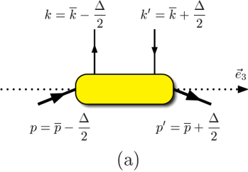
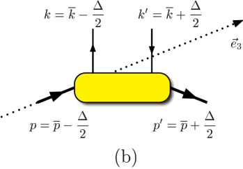
Figure 1: Illustration of two common choices to fix the longitudinal direction in the definition of the non-diagonal hadronic matrix element which defines skewed parton distributions. The flow of momenta is indicated on the lines.

As shown in Fig. 1(a) the parton emitted by the hadron has the momentum $k$, and the one absorbed has momentum $k^{\prime}$. The average parton momentum $\bar{k}$ is defined as $(k+k^{\prime})/2$, in analogy to (18), and correspondingly a momentum fraction $\bar{x}=\bar{k}^{+}/\bar{p}^{+}$ is introduced. This is Ji’s variable $x$ [3].

In an alternative parametrisation of the hadron momenta frequently found in the literature (see for instance [4]), the three-momentum of the incoming proton is chosen to lie along the ${\bf e}_{\,3}$-axis. In Fig. 1 the two different choices are illustrated. We will present our results formulated in terms of the alternative set of kinematical variables in the Appendix.

3 The unpolarised skewed quark distribution

We now turn to the derivation of the overlap representation for leading-twist SPDs. For definiteness let us consider the case of unpolarised quarks inside protons. Thus, we investigate the proton matrix element of the plus component of a flavour-diagonal bi-local quark field operator summed over colour. The generalisation to other hadrons is straightforward. Following Ji [3], we define the SPDs $H^{q}(\bar{x},\xi;t)$ and $E^{q}(\bar{x},\xi;t)$ for a quark of flavour $q$ by

$${\cal H}_{\lambda^{\prime}\lambda}^{q} \equiv \frac{1}{2\sqrt{1-\xi^{2}}}\;\sum_{c}\int\frac{{\rm d}z^{-}}{2\pi}\;e^{i\,\bar{x}\,\bar{p}^{\,+}z^{-}}\;\langle p^{\,\prime},\lambda^{\prime}|\,\overline{\psi}_{q}^{\,c}(-\bar{z}/2)\,\gamma^{+}\,\psi_{q}^{\,c}(\bar{z}/2)\,|p,\lambda\rangle$$ (24)

$$= \frac{\overline{u}(p^{\,\prime},\lambda^{\prime})\gamma^{+}u(p,\lambda)}{2\bar{p}^{\,+}\sqrt{1-\xi^{2}}}\;H^{q}(\bar{x},\xi;t)+\frac{\overline{u}(p^{\,\prime},\lambda^{\prime}){i\sigma^{+\alpha}\Delta_{\alpha}}u(p,\lambda)}{4m\,\bar{p}^{\,+}\sqrt{1-\xi^{2}}}\;E^{q}(\bar{x},\xi;t)$$

where $\lambda$, $\lambda^{\prime}$ denote the proton helicities, and $\bar{z}$ is a shorthand notation for $[0,z^{-},{\bf 0_{\perp}}]$. The link operator normally needed to render the definition (24) gauge-invariant does not appear because we choose the gauge $A^{+}=0$, which together with an integration path along the minus direction reduces the link operator to unity. With the phase conventions of the Brodsky-Lepage light-cone spinors [9] we find for the different proton helicity combinations

$${\cal H}^{q}_{++}=\phantom{-(}{\cal H}^{q}_{--}\phantom{)^{*}} = H^{q}-\frac{\xi^{2}}{1-\xi^{2}}\,E^{q}\>,$$

$${\cal H}^{q}_{-+}=-({\cal H}^{q}_{+-})^{*} = \eta\,\frac{\sqrt{t_{0}-t}}{2m}\,\frac{1}{\sqrt{1-\xi^{2}}}\,E^{q}$$ (25)

with $t_{0}$ defined in Eq. (23) and a phase factor reading

$$\eta=\frac{\Delta^{1}+i\Delta^{2}}{|{\bf\Delta}_{\perp}|}$$ (26)

for proton momenta of the form (2). In a general reference frame $\Delta^{\alpha}$ in Eq. (26) is to be replaced with $\Delta^{\alpha}-(\Delta^{+}/\bar{p}^{\,+})\,\bar{p}^{\,\alpha}$. Evaluating ${\cal H}_{\lambda^{\prime}\lambda}^{q}$ for both proton helicity flip and non-flip, one obtains the usual SPDs for quark flavour $q$, $H^{q}$ and $E^{q}$. We remark in passing that the LCWFs for proton helicity states with opposite helicity are related through a reflection about the $x$-$z$ plane [11].

A key point in our derivation of an overlap formula is the well-known observation that the bi-local quark field operator in the definition (24) can be written as a density operator in terms of the “good” LC components (see e.g. [13])

$$\overline{\psi}{}_{q}^{\,c}(-\bar{z}/2)\,\gamma^{+}\,\psi_{q}^{\,c}(\bar{z}/2)=\sqrt{2}\;\phi_{q}^{\,c\,\dagger}(-\bar{z}/2)\,\phi_{q}^{\,c}(\bar{z}/2).$$ (27)

Inserting the momentum space expansion (1) of the fields, one obtains for the Fourier transform occurring in (24)

$$\sum_{c}\int\frac{{\rm d}z^{-}}{2\pi}\;e^{i\,\bar{x}\,\bar{p}^{\,+}z^{-}}\;\overline{\psi}{}_{q}^{\,c}(-\bar{z}/2)\,\gamma^{+}\,\psi_{q}^{\,c}(\bar{z}/2)$$ (28)

$$= 2\,\int\frac{{\rm d}k^{\prime+}\,{\rm d}^{2}{\bf k}^{\prime}_{\perp}}{k^{\prime+}\,16\pi^{3}}\,\Theta(k^{\prime+})\;\int\frac{{\rm d}k^{+}\,{\rm d}^{2}{\bf k}_{\perp}}{k^{+}\,16\pi^{3}}\,\Theta(k^{+})\;\sum_{\mu,\mu^{\prime},c,c^{\prime}}\;\delta_{c^{\prime}c}$$

$$\Big{\{}\>\>\;\delta(2\bar{x}\bar{p}^{+}-k^{\prime+}-k^{+})\;b_{q}^{\dagger}(w^{\prime})\,b_{q}^{\phantom{\dagger}}(w)\,u_{+}^{\dagger}(w^{\prime})\,u_{+}(w)$$

$${}+\delta(2\bar{x}\bar{p}^{+}+k^{\prime+}+k^{+})\;d_{q}^{\phantom{\dagger}}(w^{\prime})\,d_{q}^{\dagger}(w)\,v_{+}^{\dagger}(w^{\prime})\,v_{+}(w)\phantom{\Big{\}}}$$

$${}+\delta(2\bar{x}\bar{p}^{+}+k^{\prime+}-k^{+})\;d_{q}^{\phantom{\dagger}}(w^{\prime})\,b_{q}^{\phantom{\dagger}}(w)\,v_{+}^{\dagger}(w^{\prime})\,u_{+}(w)\phantom{\Big{\}}}$$

$${}+\delta(2\bar{x}\bar{p}^{+}-k^{\prime+}+k^{+})\;b_{q}^{\dagger}(w^{\prime})\,d_{q}^{\dagger}(w)\,u_{+}^{\dagger}(w^{\prime})\,v_{+}(w)\;\Big{\}}\>,$$

a form that readily allows one to interpret the SPDs in the parton picture [14]. Which of the four terms in (28) contributes to the matrix element in (24) is determined by the positivity conditions $k^{+}\geq 0$ and $k^{\prime+}\geq 0$ for the parton momenta, together with momentum conservation, which imposes $k^{+}-k^{\prime+}=p^{+}-p^{\prime\,+}=2\xi\bar{p}^{\,+}$. For definiteness we consider the case $\xi>0$ in the following, which is relevant for the applications of the SPDs in hard processes that have so far been considered in the literature. In the region $\xi<\bar{x}<1$ the SPDs describe the emission of a quark from the nucleon with momentum fraction $\bar{x}+\xi$ and its reabsorption with $\bar{x}-\xi$. In the region $-1<\bar{x}<-\xi$ one has the emission of an antiquark from the nucleon with momentum fraction $-(\bar{x}+\xi)$ and its reabsorption with $-(\bar{x}-\xi)$. In the third region $-\xi<\bar{x}<\xi$, however, the nucleon emits a quark-antiquark pair. We will discuss the three cases separately; first we focus on the region $\xi<\bar{x}<1$ (see Fig.2). The last term in (28), going with $b^{\dagger}(w^{\prime})\,d^{\dagger}(w)$ and describing the absorption of a quark-antiquark pair, does not contribute for $\xi>0$.

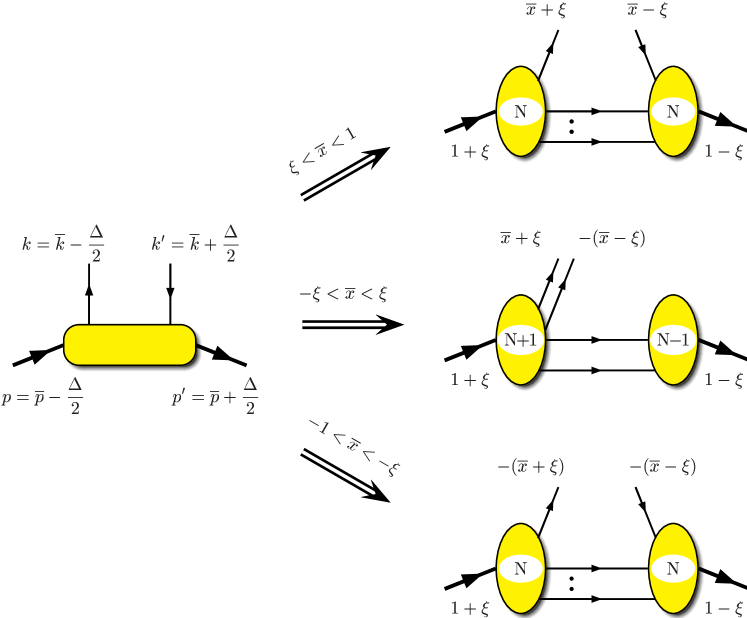
Figure 2: Overlap representations for SPDs in different kinematic regions for the case $\xi>0$. The flow of momenta is indicated on the lines. Top (bottom) right: the region $\xi<\bar{x}<1$ ($-1<\bar{x}<-\xi$), where the SPDs are given by $N\to N$ overlaps. Middle right: the central region $-\xi<\bar{x}<\xi$, where $N+1\to N-1$ overlaps are relevant.

We remark in passing that one can define distributions $H^{\bar{q}}(x,\xi;t)\equiv-H^{q}(-x,\xi;t)$ and $E^{\bar{q}}(x,\xi;t)\equiv-E^{q}(-x,\xi;t)$, which in the region $\xi<\bar{x}<1$ describe the emission and reabsorption of antiquarks and may thus be called “skewed antiquark distributions”. We will not need this here, and instead work with the distributions $H^{q}$ and $E^{q}$ and their different interpretation in the three $\bar{x}$ intervals just discussed.

3.1 The region $\xi<\bar{x}<1$

The Fock state decomposition (8) leads to a representation of the matrix element ${\cal H}_{\lambda^{\prime}\lambda}^{q}$ as a sum over contributions from separate Fock states,

$${\cal H}_{\lambda^{\prime}\lambda}^{q}=\sum_{N}{\cal H}_{\lambda^{\prime}\lambda}^{q(N\to N)}\>,$$ (29)

with

$${\cal H}_{\lambda^{\prime}\lambda}^{q(N\to N)} = \frac{1}{\sqrt{2(1-\xi^{2})}}\;\sum_{c}\sum_{\beta,\beta^{\prime}}\;\int[{\rm d}\tilde{x}]_{N}[{\rm d}^{2}\tilde{\bf k}_{\perp}]_{N}\;[{\rm d}\hat{x}^{\prime}]_{N}[{\rm d}^{2}\hat{\bf k}^{\prime}_{\perp}]_{N}\;\Psi_{N,\beta^{\prime}}^{*\,\lambda^{\prime}}(\hat{r}^{\prime})\,\Psi_{N,\beta}^{\lambda}(\tilde{r})$$ (30)

$$\times \int\frac{{\rm d}z^{-}}{2\pi}\;e^{i\,\bar{x}\,\bar{p}^{\,+}z^{-}}\,\left\langle N,\beta^{\prime};k^{\prime}_{1}\ldots k^{\prime}_{N}\right|\,\phi^{\,c\,\dagger}_{q}(-\bar{z}/2)\,\phi^{\,c}_{q}(\bar{z}/2)\,\left|N,\beta;k_{1},\ldots,k_{N}\right\rangle\;\>.\hskip 20.00003pt$$

One can now express the $N$-parton states and the bi-local quark field operator $\phi^{\,c\,\dagger}_{q}\,\phi^{\,c}_{q}$ in terms of the creation and annihilation operators, see Eqs. (10) and (28), and evaluate the resulting vacuum matrix element using the (anti)commutation relations (4) and (5).

One obtains a product of two anticommutators involving the creation and annihilation operators from $\phi^{\,c\,\dagger}_{q}\,\phi^{\,c}_{q}$, which can be rewritten as a matrix element of the field operators for the active quarks, and a product of $N-1$ (anti)commutators for the spectator partons, which is conveniently expressed through one-parton matrix elements as in (7). The quantum numbers for the active quarks and for the spectators have to match, see Eq. (7), and Eqs. (38) and (40) below, so that the Fock state labels $\beta$ and $\beta^{\prime}$ are constrained to be the same.

For identical partons in the Fock state the non-zero (anti)commutators generate a number of terms corresponding to the different possibilities to associate the partons in the initial and final states. These terms are, however, all the same because of the (anti)symmetry of the wave functions under permutations of the momenta $r_{i}$ for identical particles. The number of these terms equals the product $\sqrt{f_{N,\beta^{\prime}}f_{N,\beta}}$ of normalisation factors from the parton states times the multiplicity of the active parton. Thus, we end up with only one term, a situation which allows us to number the spectators in one specific way. We thus arrive at the following replacement of the matrix element appearing in (30)

$$\left\langle N,\beta^{\prime};k^{\prime}_{1}\ldots k^{\prime}_{N}\right|\,\phi^{\,c\,\dagger}_{q}(-\bar{z}/2)\,\phi^{\,c}_{q}(\bar{z}/2)\,\left|N,\beta;k_{1},\ldots,k_{N}\right\rangle$$ (31)

$$= \sum_{j=1}^{N}\;\frac{\langle s^{\prime}_{j};w^{\prime}_{j}|\;\phi^{\,c\,\dagger}_{q}(-\bar{z}/2)\,\phi^{\,c}_{q}(\bar{z}/2)\,|s^{\phantom{.}}_{j};w^{\phantom{.}}_{j}\rangle}{\sqrt{\hat{x}^{\prime}_{1}\ldots\hat{x}^{\prime}_{N}}\sqrt{\tilde{x}_{1}\ldots\tilde{x}_{N}\phantom{\hat{x}^{\prime}_{N}}}}\;\prod_{i=1\atop i\neq j}^{N}\langle s^{\prime}_{i};w^{\prime}_{i}|s^{\phantom{.}}_{i};w^{\phantom{.}}_{i}\rangle\;\>.$$

We now have to comment on the involved parton momenta. The parton states are characterised by their momenta and helicities, $w_{i}$. We denote momenta of partons belonging to the incoming hadron with unprimed, and the momenta of partons belonging to the outgoing hadron with primed variables. The LCWFs, on the other hand, depend on the relative momentum coordinates with respect to the parent hadron, $r_{i}$. As mentioned above, the identification of the arguments of the LCWFs is most easily done when hadron frames are chosen as frames of reference. We introduce the names “hadron-in” and “hadron-out” for frames where the incoming and outgoing hadron has zero transverse momentum, respectively. For the sake of clarity, we will here and in the following pedantically label quantities in the hadron-in (hadron-out) frame with an additional tilde (hat). We further use the name “average-frame” for a system where the hadron momenta are parameterised in the form of Eqs. (2). In order to achieve a formulation symmetric in incoming and outgoing quantities it is useful to define as auxiliary variables the averages of incoming and outgoing parton momenta in the average frame

$$\bar{k}^{\phantom{.}}_{i}=\frac{1}{2}\,(k^{\phantom{.}}_{i}+k^{\prime}_{i})\;,\qquad\bar{x}^{\phantom{.}}_{i}=\frac{\bar{k}_{i}^{+}}{\bar{p}^{+}}\>,$$ (32)

which satisfy

$$\sum_{i=1}^{N}\bar{x}_{i}=\frac{1}{\bar{p}^{+}}\,\sum_{i=1}^{N}\bar{k}^{\,+}_{i}=1\;,\qquad\sum_{i=1}^{N}\bar{\bf k}_{\perp i}=\bar{\bf p}_{\perp}={\bf 0}_{\perp}\>.$$ (33)

The parton emitted and later reabsorbed from the hadron is called the “active” parton and labelled with index $j$; all other partons $i\neq j$ play the role of “spectators”. The active parton carries a fraction $\bar{x}_{j}+\xi$ of the average plus-momentum $\bar{p}^{\,+}$ when it is taken out of the proton, and a fraction $\bar{x}^{\phantom{.}}_{j}-\xi$ when it is reinserted. The transverse momentum of the active parton is ${\bf k}_{\perp j}=\bar{\bf k}_{\perp j}-{\bf\Delta}_{\perp}/2$ before, and ${\bf k}^{\prime}_{\perp j}=\bar{\bf k}^{\phantom{.}}_{\perp j}+{\bf\Delta}^{\phantom{.}}_{\perp}/2$ after the partonic scattering process.

The arguments of the LCWF for the incoming hadron are obtained through a transverse boost (16) with parameters $b^{+}=(1+\xi)\,\bar{p}^{\,+}$ and ${\bf b}_{\perp}=-{\bf\Delta}_{\perp}/2$, which leads from the average-frame to the hadron-in frame. Likewise, a transverse boost with parameters $b^{+}=(1-\xi)\,\bar{p}^{\,+}$ and ${\bf b}_{\perp}=+{\bf\Delta}_{\perp}/2$ leads from the average-frame to the hadron-out frame. From momentum conservation and the spectator condition

$$k^{\prime}_{i}=\bar{k}^{\phantom{.}}_{i}=k^{\phantom{.}}_{i}\>,\qquad\mbox{for }i\neq j\>,$$ (34)

one obtains that the LCWF arguments for the incoming hadron (i.e., the momenta of the partons belonging to the incoming hadron in the hadron-in frame) are related to the momenta in the average-frame by

$$\tilde{x}_{i}=\frac{\bar{x}_{i}}{1+\xi}\>, \tilde{\bf k}_{\perp i}=\bar{\bf k}_{\perp i}+\frac{\bar{x}_{i}}{1+\xi}\,\frac{{\bf\Delta}_{\perp}}{2}\>,\qquad\qquad\mbox{for }i\neq j\>,$$

$$\tilde{x}_{j}=\frac{\bar{x}_{j}+\xi}{1+\xi}\>, \tilde{\bf k}_{\perp j}=\bar{\bf k}_{\perp j}-\frac{1-\bar{x}_{j}}{1+\xi}\,\frac{{\bf\Delta}_{\perp}}{2}\>.$$ (35)

Likewise, the LCWF arguments for the outgoing hadron (i.e., the momenta of the partons belonging to the outgoing hadron in the hadron-out frame) are related to the momenta in the average-frame by

$$\hat{x}^{\prime}_{i}=\frac{\bar{x}_{i}}{1-\xi}\>, \hat{\bf k}^{\prime}_{\perp i}=\bar{\bf k}^{\phantom{.}}_{\perp i}-\frac{\bar{x}_{i}}{1-\xi}\,\frac{{\bf\Delta}_{\perp}}{2}\>,\qquad\qquad\mbox{for }i\neq j\>,$$

$$\hat{x}^{\prime}_{j}=\frac{\bar{x}_{j}-\xi}{1-\xi}\>, \hat{\bf k}^{\prime}_{\perp j}=\bar{\bf k}^{\phantom{.}}_{\perp j}+\frac{1-\bar{x}_{j}}{1-\xi}\,\frac{{\bf\Delta}_{\perp}}{2}\>.$$ (36)

Using this we can express the single-particle state normalisation (7) through the LCWF arguments

$$\langle s^{\prime}_{i};w^{\prime}_{i}|s_{i};w_{i}\rangle = 16\pi^{3}\,\hat{x}^{\prime}_{i}\,\delta\left(\hat{x}^{\prime}_{i}-\tilde{x}^{\phantom{.}}_{i}\,\frac{1+\xi}{1-\xi}\right)\;$$ (37)

$$\times \delta^{(2)}\!\left(\hat{\bf k}^{\prime}_{\perp i}-\tilde{\bf k}^{\phantom{.}}_{\perp i}+\frac{\tilde{x}_{i}}{1-\xi}{\bf\Delta}^{\phantom{.}}_{\perp}\right)\;\delta_{\mu_{i}^{\prime}\mu^{\phantom{.}}_{i}}\;\delta_{s^{\prime}_{i}s_{i}^{\phantom{.}}}\;\delta_{c^{\prime}_{i}c_{i}^{\phantom{.}}}\>,$$

where the relations (3.1) and (3.1) have been used to express the variables $w_{i}$ and $w^{\prime}_{i}$ in terms of hadron frame quantities (with tilde and hat, respectively) and thus in terms of the variables occurring in the integration measures. Now we use the expansion (28) of the density operator, of which only the term with the quark operators $b^{\dagger}(w^{\prime})\,b(w)$ contributes to the matrix element here. Combined with the use of the definition of the single-quark state (2) and the anticommutation relation for the quark creation and annihilation operators this yields

$$\sum_{c}\int\frac{{\rm d}z^{-}}{2\pi}\;e^{i\,\bar{x}\,\bar{p}^{\,+}z^{-}}\,\langle s^{\prime}_{j};w^{\prime}_{j}|\,\phi^{\,c\,\dagger}_{q}(-\bar{z}/2)\,\phi^{\,c}_{q}(\bar{z}/2)\,|s^{\phantom{.}}_{j};w^{\phantom{.}}_{j}\rangle$$ (38)

$$= \frac{1}{\bar{p}^{\,+}}\;\delta(\bar{x}-\bar{x}_{j})\;u_{+}^{\dagger}(w^{\prime}_{j})\,u_{+}(w^{\phantom{.}}_{j})\;\delta_{s_{j}q}\;\delta_{s^{\prime}\!\!{}_{j}s_{j}}\,\delta_{c^{\prime}\!\!{}_{j}c_{j}}\>.$$

The argument of the $\delta$-function is simplified with the help of (32). Thus we arrive at

$${\cal H}_{\lambda^{\prime}\lambda}^{q(N\to N)} = \frac{1}{\bar{p}^{\,+}\sqrt{2(1-\xi^{2})}}\;\sqrt{\frac{1-\xi}{1+\xi}}^{\,1-N}\;\sum_{\beta,\beta^{\prime}}\;\sum_{j=1}^{N}\;\int[{\rm d}\tilde{x}]_{N}[{\rm d}^{2}\tilde{\bf k}_{\perp}]_{N}\;{\rm d}\hat{x}^{\prime}_{j}\,{\rm d}^{2}\hat{\bf k}^{\prime}_{\perp j}$$ (39)

$$\times \delta\!\left(\hat{x}^{\prime}_{j}-1+\sum_{i\neq j}\tilde{x}^{\phantom{.}}_{i}\,\frac{1+\xi}{1-\xi}\right)\;\delta^{(2)}\!\left(\hat{\bf k}^{\prime}_{\perp j}+\sum_{i\neq j}\left(\tilde{\bf k}^{\phantom{.}}_{\perp i}-\tilde{x}^{\phantom{.}}_{i}\,\frac{1+\xi}{1-\xi}{\bf\Delta}_{\perp}^{\phantom{.}}\right)\right)$$

$$\times \delta(\bar{x}-\bar{x}_{j})\;u_{+}^{\dagger}(w^{\prime}_{j})\,u_{+}(w^{\phantom{.}}_{j})\;\delta_{s_{j}q}\;\delta_{s^{\prime}\!\!{}_{j}s_{j}}\delta_{c^{\prime}\!\!{}_{j}c_{j}}\prod_{i=1\atop i\neq j}^{N}\delta_{s^{\prime}_{i}s^{\phantom{.}}_{i}}\;\delta_{\mu_{i}^{\prime}\mu^{\phantom{.}}_{i}}\;\delta_{c^{\prime}_{i}c^{\phantom{.}}_{i}}$$

$$\times \frac{\Psi_{N,\beta^{\prime}}^{*\,\lambda^{\prime}}(\hat{r}^{\prime})\,\Psi_{N,\beta}^{\lambda}(\tilde{r})}{\sqrt{\hat{x}^{\prime}_{j}\tilde{x}_{j}}}\;\>.$$

Note that the $\delta$-functions shown explicitly, together with the ones in the integration measures $[{\rm d}\tilde{x}]_{N}[{\rm d}^{2}\tilde{\bf k}_{\perp}]_{N}$, provide the relation given in (3.1) for the active quark momentum variables $\hat{x}_{j}^{\prime}$ and $\hat{\bf k}^{\prime}_{\perp j}$. The integrations over $\hat{x}_{j}^{\prime}$ and $\hat{\bf k}^{\prime}_{\perp j}$ can be carried out, and in the following the primed variables (with hat) are used as a shorthand defined by (3.1). The equality of flavours ($s^{\prime}_{j}$ and $s_{j}$) and colours ($c^{\prime}_{j}$ and $c_{j}$) is assured by the Kronecker symbols in Eq. (39), and the spinor product evaluates to

$$u_{+}^{\dagger}(w^{\prime}_{j})\,u_{+}(w_{j})=\frac{1}{\sqrt{2}}\;\bar{u}(w^{\prime}_{j})\,\gamma^{+}\,u(w_{j})=\sqrt{2\,(1-\xi^{2})\,\hat{x}^{\prime}_{j}\,\tilde{x}_{j}}\;\bar{p}^{\,+}\;\delta_{\mu_{j}^{\prime}\mu^{\phantom{.}}_{j}}\>.$$ (40)

The Kronecker-$\delta$ for the helicities in (40) could have been anticipated from the Dirac structure of the operator $\overline{\psi}{}_{q}^{\,c}\gamma^{+}\psi_{q}^{\,c}$ in (24). Defining right- and left-handed projections of the fields, $\phi_{q,R/L}^{\,c}\equiv P_{R/L}\,P_{+}\psi_{q}^{\,c}$, with $P_{R/L}=(1\pm\gamma_{5})/2$ and using $P_{\pm}\gamma_{5}=\gamma_{5}P_{\pm}$ it is easy to see that

$$\overline{\psi}{}_{q}^{\,c}\gamma^{+}\psi_{q}^{\,c}=\sqrt{2}\;\phi_{q}^{\,c\,\dagger}(P_{R}+P_{L})\,\phi_{q}^{\,c}=\sqrt{2}\;\left(\phi_{q\,R}^{\,c\,\dagger}\phi_{q\,R}^{\,c}+\phi_{q\,L}^{\,c\,\dagger}\phi_{q\,L}^{\,c}\right)\>.$$ (41)

Since for massless quarks chirality and helicity are identical, the helicities on both quark lines have to be the same.

To present our final result in a symmetric way we rewrite the integration measure in terms of the average quantities with the help of (3.1)

$$[{\rm d}\tilde{x}]_{N}=\left(\frac{1}{1+\xi}\right)^{N-1}\,[{\rm d}\bar{x}]_{N}\>,\qquad\qquad[{\rm d}^{2}\tilde{\bf k}_{\perp}]_{N}=[{\rm d}^{2}\bar{\bf k}_{\perp}]_{N}\>,$$ (42)

and arrive at the overlap representation of the quark SPD in the region $\xi<\bar{x}<1$:

$${\cal H}_{\lambda^{\prime}\lambda}^{q(N\to N)} = \sqrt{1-\xi}^{\,1-N}\sqrt{1+\xi}^{\,1-N}\;\sum_{\beta=\beta^{\prime}}\;\sum_{j}\delta_{s_{j}q}\;$$ (43)

$$\times \int[{\rm d}\bar{x}]_{N}[{\rm d}^{2}\bar{\bf k}_{\perp}]_{N}\;\delta\left(\bar{x}-\bar{x}_{j}\right)\;\Psi_{N,\beta^{\prime}}^{*\,\lambda^{\prime}}(\hat{r}^{\prime})\,\Psi_{N,\beta}^{\lambda}(\tilde{r})\>,$$

with the arguments $\tilde{r}$ ($\hat{r}^{\prime}$) of the LCWF for the incoming (outgoing) proton being related to the integration variables $\bar{x}_{i}$ and $\bar{\bf k}_{\perp i}$ by (3.1) and (3.1), respectively. Summation over $N$ leads to the full expression of ${\cal H}_{\lambda^{\prime}\lambda}^{q}$ in the region $\xi<\bar{x}<1$. Alternatively, as we discussed in Sect. 2, one could use $N$-parton Fock states that are coupled to be colourless and carry the quantum numbers of the hadron. Normalising these states in analogy to Eq. (11) and denoting the associated LCWFs by $\widetilde{\Psi}_{N,\tilde{\beta}}$, one would obtain an overlap $\widetilde{\Psi}^{*}{}_{\!\!\!N,\tilde{\beta^{\prime}}}\,\widetilde{\Psi}_{N,\tilde{\beta}}$ summed over $\tilde{\beta}=\tilde{\beta}^{\prime}$, just as in (43). This simple structure is owed to the constraint $\beta=\beta^{\prime}$ in (43) and will no longer appear in the region $-\xi<\bar{x}<\xi$, see Eq. (55).

3.2 The region $-1<\bar{x}<-\xi$

For active antiquarks the derivation of the overlap representation of the SPDs goes in full analogy to the one we have just given. Differences appear when the Fourier decomposition (28) is used to yield the analogue of Eq. (38), since it is now the term with $d(w^{\prime})\,d^{\dagger}(w)$ that contributes. Exchanging the order of the annihilation and creation operator gives an overall minus sign, and the $\delta$-function in the analogue of Eq. (38) now gives the constraint $\bar{x}_{j}=-\bar{x}$. The final result for the region $-1<\bar{x}<-\xi$ is

$${\cal H}_{\lambda^{\prime}\lambda}^{q(N\to N)} = {}-\sqrt{1-\xi}^{\,1-N}\sqrt{1+\xi}^{\,1-N}\;\sum_{\beta=\beta^{\prime}}\;\sum_{j}\delta_{\bar{s}_{j}q}\;$$ (44)

$$\times \int[{\rm d}\bar{x}]_{N}[{\rm d}^{2}\bar{\bf k}_{\perp}]_{N}\;\delta\left(\bar{x}+\bar{x}_{j}\right)\;\Psi_{N,\beta^{\prime}}^{*\,\lambda^{\prime}}(\hat{r}^{\prime})\,\Psi_{N,\beta}^{\lambda}(\tilde{r})\>,$$

with the LCWF arguments $\tilde{r}$ and $\hat{r}^{\prime}$ given by (3.1) and (3.1), respectively

3.3 The region $-\xi<\bar{x}<\xi$

Let us now consider the kinematical range $-\xi<\bar{x}<\xi$. As mentioned above, we restrict ourselves to the case $\xi>0$. Therefore, the quark SPDs in this region describe the emission of a quark-antiquark pair from the initial proton. In the Fock state decompositions of the initial and final protons we thus have to consider only terms where the initial state has the same parton content as the final state plus one additional quark-antiquark pair. We thus have

$${\cal H}_{\lambda^{\prime}\lambda}^{q}=\sum_{N}{\cal H}_{\lambda^{\prime}\lambda}^{q(N+1\to N-1)}$$ (45)

as opposed to (29). This particular type of overlap was recently identified in [15] in the context of transition form factors between heavy and light mesons.

Starting from the definition (24) of SPDs for quarks of flavour $q$ and replacing the hadronic states by their Fock state decomposition (8), the contribution of the $N+1\to N-1$ transition to the matrix element ${\cal H}_{\lambda^{\prime}\lambda}^{q}$ is found to be

$${\cal H}_{\lambda^{\prime}\lambda}^{q(N+1\to N-1)}=\frac{1}{\sqrt{2(1-\xi^{2})}}\;\sum_{c}\sum_{\beta,\beta^{\prime}}\;\int[{\rm d}\tilde{x}]_{N+1}[{\rm d}^{2}\tilde{\bf k}_{\perp}]_{N+1}\;[{\rm d}\hat{x}^{\prime}]_{N-1}[{\rm d}^{2}\hat{\bf k}^{\prime}_{\perp}]_{N-1}\;$$ (46)

$$\times \Psi_{N-1,\beta^{\prime}}^{*\,\lambda^{\prime}}(\hat{r}^{\prime})\,\Psi_{N+1,\beta}^{\lambda}(\tilde{r})\int\frac{{\rm d}z^{-}}{2\pi}\;e^{i\,\bar{x}\,\bar{p}^{\,+}z^{-}}$$

$$\times \left\langle N-1,\beta^{\prime};k^{\prime}_{1}\ldots k^{\prime}_{N-1}\right|\,\phi^{\,c\,\dagger}_{q}(-\bar{z}/2)\,\phi_{q}^{\,c}(\bar{z}/2)\,\left|\phantom{k^{\prime}_{N-1}}N+1,\beta;k_{1},\ldots,k_{N+1}\right\rangle\;\>.\hskip 20.00003pt$$

Using again the (anti)commutation relations for the creation and annihilation operators the partonic matrix element can be replaced by

$$\left\langle N-1,\beta^{\prime};k^{\prime}_{1}\ldots k^{\prime}_{N-1}\right|\,\phi^{\,c\,\dagger}_{q}(-\bar{z}/2)\,\phi_{q}^{\,c}(\bar{z}/2)\,\left|\phantom{k^{\prime}_{N-1}}N+1,\beta;k_{1},\ldots,k_{N+1}\right\rangle\;$$ (47)

$$= \sum_{j,j^{\prime}=1}^{N+1}\;\frac{1}{\sqrt{n_{j}n_{j^{\prime}}\rule{0.0pt}{6.99997pt}}}\;\frac{\langle 0|\,\phi^{\,c\,\dagger}_{q}(-\bar{z}/2)\,\phi_{q}^{\,c}(\bar{z}/2)\,|s_{j},w_{j};s_{j^{\prime}},w_{j^{\prime}}\rangle}{\sqrt{\hat{x}^{\prime}_{1}\ldots\hat{x}^{\prime}_{N-1}}\sqrt{\tilde{x}_{1}\ldots\tilde{x}_{N+1}\phantom{\hat{x}^{\prime}_{N-1}}}}\;\prod_{i=1\atop i\neq j,j^{\prime}}^{N+1}\langle s^{\prime}_{i};w^{\prime}_{i}|s^{\phantom{.}}_{i};w^{\phantom{.}}_{i}\rangle\>,\hskip 20.00003pt$$

where we label the active quark-antiquark pair with indices $j$ for the quark and $j^{\prime}$ for the antiquark, and write $|s_{j},w_{j};s_{j^{\prime}},w_{j^{\prime}}\rangle=b^{\dagger}_{s_{j}}(w_{j})\,d^{\dagger}_{s_{j^{\prime}}}(w_{j^{\prime}})\,|0\rangle$ for the corresponding two-parton state. The sum over $\beta$ and $\beta^{\prime}$ now runs over combinations where flavour, helicity (and colour) of all spectators match. $n_{j}$ ($n_{j^{\prime}}$) is the number of (anti)quarks in the initial proton wave function $\Psi_{N+1,\beta}^{\lambda}(r)$ with the same discrete quantum numbers as the active (anti)quark. These factors appear since the product $\sqrt{f_{N+1,\beta}\,f_{N-1,\beta^{\prime}}}$ of normalisation factors from the parton states (10) is not equal to the number of possibilities to associate the partons in the initial and final proton, in contrast to the situation in the regions discussed so far.

To simplify the notation we use the same numbering for the spectator partons in the LCWFs of the initial and final state proton. Thus the $N-1$ partons in the outgoing proton are numbered not as $i=1,\ldots,N-1$, but as $i=1,\ldots,N+1$ with $j$ and $j^{\prime}$ omitted. From the spectator momenta $k^{\phantom{.}}_{i}$ and $k^{\prime}_{i}$ ($i\neq j,j^{\prime}$) we again form the auxiliary variables defined in Eq. (32). For $j$ and $j^{\prime}$ we introduce

$$\bar{k}_{j}=\frac{1}{2}\,(k_{j}-k_{j^{\prime}})\;,\qquad\bar{x}_{j}=\frac{\bar{k}_{j}^{+}}{\bar{p}^{+}}\>,$$ (48)

which is half the relative momentum (and momentum fraction) between the active quark and antiquark. It can as well be viewed as the average of $k_{j}$ and the reversed momentum $k_{j^{\prime}}$ (i.e., $-k_{j^{\prime}}$), in complete analogy with the definitions (32). From momentum conservation and the spectator condition

$$k^{\prime}_{i}=\bar{k}_{i}^{\phantom{.}}=k_{i}^{\phantom{.}}\>,\qquad\mbox{for }i\neq j,j^{\prime}$$ (49)

we now obtain that the LCWF arguments for the incoming hadron are related to the parton momenta in the average-frame by

$$\tilde{x}_{i}=\frac{\bar{x}_{i}}{1+\xi}\>, \tilde{\bf k}_{\perp i}=\bar{\bf k}_{\perp i}+\frac{\bar{x}_{i}}{1+\xi}\,\frac{{\bf\Delta}^{\phantom{.}}_{\perp}}{2}\>,\qquad\qquad\mbox{for }i\neq j,j^{\prime}\>,$$

$$\tilde{x}_{j}=\frac{\bar{x}_{j}+\xi}{1+\xi}\>, \tilde{\bf k}_{\perp j}=\bar{\bf k}_{\perp j}-\frac{1-\bar{x}_{j}}{1+\xi}\,\frac{{\bf\Delta}^{\phantom{.}}_{\perp}}{2}\>,$$

$$\tilde{x}_{j^{\prime}}=-\frac{\bar{x}_{j}-\xi}{1+\xi}\>, \tilde{\bf k}_{\perp j^{\prime}}=-\bar{\bf k}_{\perp j}-\frac{1+\bar{x}_{j}}{1+\xi}\,\frac{{\bf\Delta}^{\phantom{.}}_{\perp}}{2}\>,$$ (50)

and that the LCWF arguments for the outgoing hadron are given by

$$\hat{x}^{\prime}_{i}=\frac{\bar{x}_{i}}{1-\xi}\>, \hat{\bf k}^{\prime}_{\perp i}=\bar{\bf k}^{\phantom{.}}_{\perp i}-\frac{\bar{x}_{i}}{1-\xi}\,\frac{{\bf\Delta}^{\phantom{.}}_{\perp}}{2}\>,\qquad\qquad\mbox{for }i\neq j,j^{\prime}\>.$$ (51)

The relations (3.3) and (51) can be used to write $\langle s^{\prime};w^{\prime}|s;w\rangle$ again as in Eq. (37), and for the evaluation of the matrix element of the active quark-antiquark pair we insert the expansion (28) of the density operator, now keeping only the term with $d(w^{\prime})\,b(w)$. We then use the definition of the two-parton state given after (47), and the anticommutation relations (4) to write

$$\sum_{c}\int\frac{{\rm d}z^{-}}{2\pi}\;e^{i\,\bar{x}\,\bar{p}^{\,+}z^{-}}\,\langle 0|\,\phi^{\,c\,\dagger}_{q}(-\bar{z}/2)\,\phi^{\,c}_{q}(\bar{z}/2)\,|s_{j},w_{j};s_{j^{\prime}},w_{j^{\prime}}\rangle$$ (52)

$$= \frac{1}{\bar{p}^{\,+}}\;\delta(\bar{x}-\bar{x}_{j})\;v_{+}^{\dagger}(w_{j^{\prime}})\,u_{+}(w^{\phantom{.}}_{j})\;\delta_{{\bar{s}}_{j^{\prime}}s^{\phantom{.}}_{j}}\;\delta_{s^{\phantom{.}}_{j}q}\;\delta_{{c}_{j^{\prime}}c^{\phantom{.}}_{j}}\>.$$

Putting the pieces together we arrive at

$${\cal H}_{\lambda^{\prime}\lambda}^{q(N+1\to N-1)}=\frac{1}{\bar{p}^{\,+}\sqrt{2(1-\xi^{2})}}\;\sqrt{\frac{1-\xi}{1+\xi}}^{\,1-N}\;\sum_{\beta,\beta^{\prime}}\;\sum_{j,j^{\prime}=1}^{N+1}\frac{1}{\sqrt{n_{j}n_{j^{\prime}}\rule{0.0pt}{6.99997pt}}}$$ (53)

$$\times \int[{\rm d}\tilde{x}]_{N+1}[{\rm d}^{2}\tilde{\bf k}_{\perp}]_{N+1}\,16\pi^{3}\;\delta\!\left(1-\frac{1+\xi}{1-\xi}\sum_{i=1\atop i\neq j,j^{\prime}}^{N+1}\tilde{x}_{i}\right)\;\delta^{(2)}\!\left(\frac{{\bf\Delta}_{\perp}}{1+\xi}-\sum_{i=1\atop i\neq j,j^{\prime}}^{N+1}\tilde{\bf k}_{\perp i}\right)$$

$$\times \delta(\bar{x}-\bar{x}_{j})\;v_{+}^{\dagger}(w_{j^{\prime}})\,u_{+}(w_{j})\;\delta_{{\bar{s}}_{j^{\prime}}s^{\phantom{.}}_{j}}\;\delta_{s^{\phantom{.}}_{j}q}\;\delta_{{c}_{j^{\prime}}c^{\phantom{.}}_{j}}\;\prod_{i=1\atop i\neq j,j^{\prime}}^{N+1}\delta_{s^{\prime}_{i}s^{\phantom{.}}_{i}}\;\delta_{\mu_{i}^{\prime}\mu^{\phantom{.}}_{i}}\;\delta_{c^{\prime}_{i}c^{\phantom{.}}_{i}}$$

$$\times \frac{\Psi_{N-1,\beta^{\prime}}^{*\,\lambda^{\prime}}(\hat{r}^{\prime})\,\Psi_{N+1,\beta}^{\lambda}(\tilde{r})}{\sqrt{\tilde{x}_{j}\tilde{x}_{j^{\prime}}}}\>.\hskip 20.00003pt$$

The spinor product occurring is

$$v_{+}^{\dagger}(w_{j^{\prime}})\,u_{+}(w_{j})=\frac{1}{\sqrt{2}}\;\bar{v}(w_{j^{\prime}})\,\gamma^{+}\,u(w_{j})=\sqrt{2\,\tilde{x}_{j}\,\tilde{x}_{j^{\prime}}}\;(1+\xi)\;\bar{p}^{\,+}\;\delta_{\mu_{j^{\prime}}-\mu^{\phantom{.}}_{j}}\>.$$ (54)

The integrations over $\tilde{x}_{j^{\prime}}$ and $\tilde{\bf k}_{\perp j^{\prime}}$ can be carried out, and by rewriting the remaining integrations in terms of the auxiliary variables we arrive at the overlap representation of ${\cal H}_{\lambda^{\prime}\lambda}^{q}$ in the region $-\xi<\bar{x}<\xi$ for the $N+1\to N-1$ transition:

$${\cal H}_{\lambda^{\prime}\lambda}^{q(N+1\to N-1)} = \sqrt{1-\xi}^{\,2-N}\sqrt{1+\xi}^{\,-N}\;\sum_{\beta,\beta^{\prime}}\;\sum_{j,j^{\prime}=1}^{N+1}\frac{1}{\sqrt{n_{j}n_{j^{\prime}}\rule{0.0pt}{6.99997pt}}}\;\delta_{{\bar{s}}_{j^{\prime}}s^{\phantom{.}}_{j}}\;\delta_{s^{\phantom{.}}_{j}q}\;\delta_{\mu_{j^{\prime}}-\mu^{\phantom{.}}_{j}}\,\delta_{{c}_{j^{\prime}}c^{\phantom{.}}_{j}}\;$$ (55)

$$\times \prod_{i=1\atop i\neq j,j^{\prime}}^{N+1}\delta_{\mu_{i}^{\prime}\mu^{\phantom{.}}_{i}}\;\delta_{s^{\prime}_{i}s^{\phantom{.}}_{i}}\;\delta_{c^{\prime}_{i}c^{\phantom{.}}_{i}}\;\int{\rm d}\bar{x}_{j}\prod_{i=1\atop i\neq j,j^{\prime}}^{N+1}{\rm d}\bar{x}_{i}\;\delta\left(1-\xi-\sum_{i=1\atop i\neq j,j^{\prime}}^{N+1}\bar{x}_{i}\right)\;$$

$$\times \int{\rm d}^{2}\bar{\bf k}_{\perp j}\prod_{i=1\atop i\neq j,j^{\prime}}^{N+1}{\rm d}^{2}\bar{\bf k}_{\perp i}\;(16\pi^{3})^{1-N}\;\delta^{(2)}\!\left(\frac{{\bf\Delta}_{\perp}}{2}-\sum_{i=1\atop i\neq j,j^{\prime}}^{N+1}\bar{\bf k}_{\perp i}\right)$$

$$\times \delta\left(\bar{x}-\bar{x}_{j}\right)\;\Psi_{N-1,\beta^{\prime}}^{*\,\lambda^{\prime}}(\hat{r}^{\prime})\,\Psi_{N+1,\beta}^{\lambda}(\tilde{r})\>,\phantom{\prod_{i=1\atop i\neq j,j^{\prime}}^{N+1}}$$

The arguments $\tilde{r}$ and $\hat{r}^{\prime}$ of the wave functions are given in terms of $\bar{x}_{i}$ and $\bar{\bf k}_{\perp i}$ by (3.3) and (51), and $n_{j}$, $n_{j^{\prime}}$ are defined after Eq. (46). As was to be expected, the operator $\sum_{c}\bar{\psi}^{\,c}_{q}\gamma^{+}\psi_{q}^{\,c}$ in (24) projects out colour singlet $q\bar{q}$ pairs with total helicity zero in the initial proton LCWF.

At this point we see the advantage of our method to start from the parton states (10). If one uses colour neutral parton states with the quantum numbers of the hadron under investigation, one has in general to rearrange their colour coupling to ensure that the active $q\bar{q}$ pair is in a colour singlet state, and a combinatorial factor different from $1/\sqrt{\rule{0.0pt}{6.02773pt}n_{j}n_{j^{\prime}}}$ will then appear in (55). Although such a procedure should be possible using appropriate group theoretical methods (see e.g. [16]), we have not pursued this point here.

4 Quark polarisation and gluons

4.1 The polarised skewed quark distribution

We now turn to the polarised skewed quark distributions, $\widetilde{H}^{q}(\bar{x},\xi;t)$ and $\widetilde{E}^{q}(\bar{x},\xi;t)$, defined by the Fourier transform of the axial vector matrix element

$$\widetilde{\cal H}_{\lambda^{\prime}\lambda}^{q} \equiv \frac{1}{2\,\sqrt{1-\xi^{2}}}\;\sum_{c}\int\frac{{\rm d}z^{-}}{2\pi}\;e^{i\,\bar{x}\,\bar{p}^{\,+}z^{-}}\;\langle p^{\,\prime},\lambda^{\prime}|\,\overline{\psi}{}_{q}^{\,c}(-\bar{z}/2)\,\gamma^{+}\gamma_{5}\,\psi_{q}^{\,c}(\bar{z}/2)\,|p,\lambda\rangle$$ (56)

$$= \frac{\overline{u}(p^{\,\prime},\lambda^{\prime})\gamma^{+}\gamma_{5}u(p,\lambda)}{2\bar{p}^{\,+}\sqrt{1-\xi^{2}}}\;\widetilde{H}^{q}(\bar{x},\xi;t)+\frac{\overline{u}(p^{\,\prime},\lambda^{\prime})\Delta^{+}\gamma_{5}u(p,\lambda)}{4m\,\bar{p}^{\,+}\sqrt{1-\xi^{2}}}\;\widetilde{E}^{q}(\bar{x},\xi;t)\>.$$

For the different proton helicity combinations we now find

$$\widetilde{\cal H}^{q}_{++}=-\phantom{(}\widetilde{\cal H}^{q}_{--}\phantom{)^{*}} = \widetilde{H}^{q}-\frac{\xi^{2}}{1-\xi^{2}}\,\widetilde{E}^{q}\>,$$

$$\widetilde{\cal H}^{q}_{-+}=\phantom{-}(\widetilde{\cal H}^{q}_{+-})^{*} = \eta\,\frac{\sqrt{t_{0}-t}}{2m}\,\frac{\xi}{\sqrt{1-\xi^{2}}}\,\widetilde{E}^{q}\>.$$ (57)

The derivation of an overlap formula goes along the same lines as for the unpolarised quark SPDs. We just need the appropriate conversion of the quark field operators into a density of LC fields. Expressing the axial vector operator in terms of the left- and right-handed projections we obtain

$$\overline{\psi}{}_{q}^{\,c}\gamma^{+}\gamma_{5}\psi^{\,c}_{q}=\sqrt{2}\;\phi^{\,c\,\dagger}_{q}\gamma_{5}\phi^{\,c}_{q}=\sqrt{2}\;\left(\phi^{\,c\,\dagger}_{q\,R}\phi^{\,c}_{q\,R}-\phi^{\,c\,\dagger}_{q\,L}\phi^{\,c}_{q\,L}\right)\>.$$ (58)

Compared to (41) the difference of density operators for left- and right-handed projections now appears. Repeating all steps in the derivation of (43) one finds the overlap representation of the contribution of the $N$ particle Fock state to the SPD for a polarised quark of flavour $q$ in the region $\xi<\bar{x}<1$

$$\widetilde{\cal H}_{\lambda^{\prime}\lambda}^{q(N\to N)} = \sqrt{1-\xi}^{\,1-N}\sqrt{1+\xi}^{\,1-N}\;\sum_{\beta=\beta^{\prime}}\;\sum_{j}\mbox{sign}(\mu_{j})\;\delta_{s_{j}q}\;$$ (59)

$$\times \int[{\rm d}\bar{x}]_{N}[{\rm d}^{2}\bar{\bf k}_{\perp}]_{N}\;\delta\left(\bar{x}-\bar{x}_{j}\right)\;\Psi_{N,\beta^{\prime}}^{*\,\lambda^{\prime}}(\hat{r}^{\prime})\,\Psi_{N,\beta}^{\lambda}(\tilde{r})\>,$$

where the arguments of the LCWFs are again given by the relations (3.1) and (3.1). The only difference between the RHS of (59) and the RHS of (43) is the sign-function of the helicity of the active quark. Summation over all Fock states as in (29) leads to the final result. In the region $-1<\bar{x}<-\xi$ one has

$$\widetilde{\cal H}_{\lambda^{\prime}\lambda}^{q(N\to N)} = \sqrt{1-\xi}^{\,1-N}\sqrt{1+\xi}^{\,1-N}\;\sum_{\beta=\beta^{\prime}}\;\sum_{j}\mbox{sign}(\mu_{j})\;\delta_{\bar{s}_{j}q}\;$$ (60)

$$\times \int[{\rm d}\bar{x}]_{N}[{\rm d}^{2}\bar{\bf k}_{\perp}]_{N}\;\delta\left(\bar{x}+\bar{x}_{j}\right)\;\Psi_{N,\beta^{\prime}}^{*\,\lambda^{\prime}}(\hat{r}^{\prime})\,\Psi_{N,\beta}^{\lambda}(\tilde{r})\>.$$

In contrast to Eq. (44) there is no global minus sign here, because $\mbox{sign}(\mu_{j})$ refers to the antiquark helicity, which is minus the chirality selected by the operator (58). The non-diagonal overlap $\widetilde{\cal H}_{\lambda^{\prime}\lambda}^{q(N+1\to N-1)}$ in the central region is identical to (55) except for an additional factor $\mbox{sign}(\mu_{j})$, as appears in (59), where $\mu_{j}$ refers to the helicity of the active quark.

4.2 The unpolarised skewed gluon distribution

The unpolarised skewed gluon distributions $H^{g}(\bar{x},\xi;t)$ and $E^{g}(\bar{x},\xi;t)$ are defined from the Fourier transform of a hadronic matrix element involving two gluon field strength tensors at a light-like distance:

$${\cal H}^{g}_{\lambda^{\prime}\lambda} \equiv \frac{-g_{\perp\,\alpha^{\prime}\alpha}}{\bar{p}^{\,+}\sqrt{1-\xi^{2}}}\;\sum_{c}\int\frac{{\rm d}z^{-}}{2\pi}e^{i\bar{x}\,\bar{p}^{\,+}z^{-}}\;\langle p^{\prime},\lambda^{\prime}|\,G_{c}^{+\alpha^{\prime}}(-\bar{z}/2)\,G_{c}^{+\alpha}(\bar{z}/2)\,|p,\lambda\rangle$$ (61)

$$= \frac{\overline{u}(p^{\prime},\lambda^{\prime})\gamma^{+}u(p,\lambda)}{2\bar{p}^{\,+}\sqrt{1-\xi^{2}}}\;H^{g}(\bar{x},\xi;t)+\frac{\overline{u}(p^{\prime},\lambda^{\prime})i\sigma^{+\alpha}\Delta_{\alpha}u(p,\lambda)}{4m\,\bar{p}^{\,+}\sqrt{1-\xi^{2}}}\;E^{g}(\bar{x},\xi;t)$$

with the transverse metric tensor $g_{\perp}^{\alpha^{\prime}\alpha}$, which has $g_{\perp}^{11}=g_{\perp}^{22}=-1$ as only non-zero elements. Again the link operator is not displayed. Notice that in the $A^{+}=0$ gauge the relation $G_{c}^{+\alpha}=\partial^{+}A_{c}^{\alpha}$ provides a simple transition from field strengths to potentials. The normalisation in Eq. (61) is chosen such that in the forward limit the SPD $H^{g}$ is related to the ordinary gluon distribution $g(x)$ (for the definition see [17]) by

$$H^{g}(\bar{x},\xi=0;t=0)=\bar{x}\,g(\bar{x})\>.$$ (62)

The derivation of an overlap formula proceeds in close analogy to the one for the quark SPDs. There is only one technical point we have to comment on. From the expansion (2) of the transverse components of the gluon field operators in momentum space, one encounters a combination of polarisation vectors for the active gluons, which in the region $\xi<\bar{x}<1$ reads

$$\epsilon^{*\,\alpha^{\prime}}(w^{\prime}_{j})\,\epsilon^{\alpha}(w_{j})\>,$$ (63)

and is to be contracted with $g_{\perp\,\alpha^{\prime}\alpha}$. In a frame where the active on-shell gluon in the incoming hadron has no transverse momentum, its polarisation vector is purely transverse and does not depend on its momentum:

$$\epsilon(k^{+}_{j},{\bf k}_{\perp j}=0,\mu_{j})=\left[\;0\;,\;0\;,\;{\vec{\epsilon}}_{\perp}(\mu_{j})\;\right]\>,$$ (64)

where ${\vec{\epsilon}}_{\perp}(\mu)=(-\mu,-i)/\sqrt{2}$. A transverse boost from this frame to the hadron-in frame leaves the transverse components unchanged. This is because the plus component of the polarisation vector in the starting frame is zero. The plus component itself remains zero by virtue of the definition of a transverse boost. The transformation produces a non-zero minus component which we do not have to specify, since the polarisation vector will be contracted with a transverse tensor. A similar argument can be given for the polarisation vector of the reabsorbed gluon, starting in a frame where its momentum has no transverse component and applying an appropriate transverse boost. Explicitly, we get

$$\epsilon^{*\,\alpha^{\prime}}(w^{\prime}_{j})\,\epsilon^{\alpha}(w_{j}) = -\frac{1}{2}\left(g_{\perp}^{\alpha^{\prime}\alpha}-\mbox{sign}(\mu_{j})\,i\,\varepsilon_{\perp}^{\alpha^{\prime}\alpha}\right)\,\delta_{\mu^{\prime}_{j}\mu^{\phantom{.}}_{j}}-\frac{1}{2}\;t_{\perp}^{\,\alpha^{\prime}\alpha}\;\delta_{\mu^{\prime}_{j}-\mu^{\phantom{.}}_{j}}$$ (65)

$$+\mbox{``non-transverse''}\rule{0.0pt}{12.91663pt}\>,$$

where $\varepsilon_{\perp}^{12}=-\varepsilon_{\perp}^{21}=1$, $t_{\perp}^{\,11}=-t_{\perp}^{\,22}=1$, and $t_{\perp}^{\,12}=t_{\perp}^{\,21}=i\mu_{j}$, while all other components of these tensors are zero. The term “non-transverse” stands for a matrix with vanishing matrix elements in the transverse sub-space. Neither this matrix nor $t_{\perp}^{\alpha^{\prime}\alpha}$ contribute when contracted with transverse tensors $g_{\perp\,\alpha^{\prime}\alpha}$ and $\varepsilon_{\perp\,\alpha^{\prime}\alpha}$, which occur in the definition of the unpolarised and polarised skewed gluon distributions.

The final result for the overlap representation for the unpolarised gluon SPD in the region $\xi<\bar{x}<1$ is

$${\cal H}_{\lambda^{\prime}\lambda}^{g(N\to N)} = \sqrt{\bar{x}^{2}-\xi^{2}}\;\sqrt{1-\xi}^{\,1-N}\sqrt{1+\xi}^{\,1-N}\;\sum_{\beta=\beta^{\prime}}\;\sum_{j}\delta_{s_{j}g}\;$$ (66)

$$\times \int[{\rm d}\bar{x}]_{N}[{\rm d}^{2}\bar{\bf k}_{\perp}]_{N}\;\delta\left(\bar{x}-\bar{x}_{j}\right)\;\Psi_{N,\beta^{\prime}}^{*\,\lambda^{\prime}}(\hat{r}^{\prime})\,\Psi_{N,\beta}^{\lambda}(\tilde{r})\,\>,$$

where the sum over $j$ runs over all gluons, and the arguments, $\tilde{r}$ and $\hat{r}^{\prime}$ of the LCWFs are related to the auxiliary variables $\bar{x}_{i}$ and $\bar{\bf k}_{\perp i}$ by the relations (3.1) and (3.1).

For the region $-1<\bar{x}<-\xi$ the gluon SPDs can be readily obtained from (66) with the observation that $H^{g}$ and $E^{g}$ are even functions in $\bar{x}$, since the gluon is its own antiparticle.

In the region $-\xi<\bar{x}<\xi$ the gluon SPDs describe the emission of two gluons from the initial proton. In the Fock state decomposition, therefore, we have to consider $N+1\to N-1$ transitions, where the initial state has the same parton content as the final state plus two additional gluons. In the derivation of an overlap representation one encounters a combination of polarisation vectors, which can be evaluated exactly along the lines discussed above as

$$\epsilon^{\alpha^{\prime}}(w_{j^{\prime}})\,\epsilon^{\alpha}(w_{j}) = \frac{1}{2}\,\left(g_{\perp}^{\alpha^{\prime}\alpha}-\mbox{sign}(\mu_{j})\,i\,\varepsilon_{\perp}^{\alpha^{\prime}\alpha}\right)\,\delta_{\mu_{j^{\prime}}-\mu^{\phantom{.}}_{j}}+\frac{1}{2}\;t_{\perp}^{\,\alpha^{\prime}\alpha}\;\delta_{\mu_{j^{\prime}}\mu^{\phantom{.}}_{j}}$$ (67)

$$+\mbox{``non-transverse''}\rule{0.0pt}{12.91663pt}\>.$$

Accordingly, the overlap representation of ${\cal H}^{g}_{\lambda^{\prime}\lambda}$ in the region $-\xi<\bar{x}<\xi$ for the $N+1\to N-1$ transition becomes

$${\cal H}_{\lambda^{\prime}\lambda}^{g(N+1\to N-1)} = -\sqrt{\xi^{2}-\bar{x}^{2}}\;\sqrt{1-\xi}^{\,2-N}\sqrt{1+\xi}^{\,-N}$$ (68)

$$\times \sum_{\beta,\beta^{\prime}}\;\sum_{j,j^{\prime}=1\atop j\neq j^{\prime}}^{N+1}\frac{1}{\sqrt{n_{j}n_{j^{\prime}}\rule{0.0pt}{6.99997pt}}}\;\delta_{s_{j^{\prime}}s_{j}}\;\delta_{s_{j}g}\;\delta_{\mu_{j^{\prime}}-\mu^{\phantom{.}}_{j}}\,\delta_{\bar{c}_{j^{\prime}}c_{j}}\;\prod_{i=1\atop i\neq j,j^{\prime}}^{N+1}\delta_{s^{\prime}_{i}s^{\phantom{.}}_{i}}\;\delta_{\mu_{i}^{\prime}\mu^{\phantom{.}}_{i}}\;\delta_{c^{\prime}_{i}c^{\phantom{.}}_{i}}\;$$

$$\times \int{\rm d}\bar{x}_{j}\prod_{i=1\atop i\neq j,j^{\prime}}^{N+1}{\rm d}\bar{x}_{i}\;\delta\left(\sum_{i=1\atop i\neq j,j^{\prime}}^{N+1}\bar{x}_{i}-(1-\xi)\right)\;$$

$$\times \int{\rm d}^{2}\bar{\bf k}_{\perp j}\prod_{i=1\atop i\neq j,j^{\prime}}^{N+1}{\rm d}^{2}\bar{\bf k}_{\perp i}\;(16\pi^{3})^{1-N}\;\delta^{(2)}\!\left(\sum_{i=1\atop i\neq j,j^{\prime}}^{N+1}\bar{\bf k}_{\perp i}-\frac{{\bf\Delta}_{\perp}}{2}\right)$$

$$\times \delta\left(\bar{x}-\bar{x}_{j}\right)\;\Psi_{N-1,\beta^{\prime}}^{*\,\lambda^{\prime}}(\hat{r}^{\prime})\,\Psi_{N+1,\beta}^{\lambda}(\tilde{r})\>,\phantom{\prod_{i=1\atop i\neq j,j^{\prime}}^{N+1}}$$

where both $j$ and $j^{\prime}$ run over all gluons. The sum over $\beta$ and $\beta^{\prime}$ runs over combinations where flavour and colour of all spectators match. The arguments $\tilde{r}$ and $\hat{r}^{\prime}$ of the wave functions are given in terms of $\bar{x}_{i}$ and $\bar{\bf k}_{\perp i}$ by (3.3) and (51).

We finally remark that compared with the quark SPDs, the overlap representation for the case of gluons has an extra factor of $\sqrt{|\bar{x}^{2}-\xi^{2}|}$ in all regions of $\bar{x}$.

4.3 The polarised skewed gluon distribution

The polarised gluon SPDs $\widetilde{H}^{g}(\bar{x},\xi;t)$ and $\widetilde{E}^{g}(\bar{x},\xi;t)$ are defined from

$$\widetilde{\cal H}^{g}_{\lambda^{\prime}\lambda} \equiv \frac{i\,\varepsilon^{\phantom{.}}_{\perp\,\alpha^{\prime}\alpha}}{\bar{p}^{\,+}\sqrt{1-\xi^{2}}}\;\sum_{c}\int\frac{{\rm d}z^{-}}{2\pi}e^{i\bar{x}\,\bar{p}^{\,+}z^{-}}\;\langle p^{\,\prime},\lambda^{\prime}|\,G_{c}^{+\alpha^{\prime}}(-\bar{z}/2)\,G_{c}^{+\alpha}(\bar{z}/2)\,|p,\lambda\rangle$$ (69)

$$= \frac{\overline{u}(p^{\,\prime},\lambda^{\prime})\gamma^{+}\gamma_{5}u(p,\lambda)}{2\bar{p}^{\,+}\sqrt{1-\xi^{2}}}\;\widetilde{H}^{g}(\bar{x},\xi;t)+\frac{\overline{u}(p^{\,\prime},\lambda^{\prime})\Delta^{+}\gamma_{5}u(p,\lambda)}{4m\,\bar{p}^{\,+}\sqrt{1-\xi^{2}}}\;\widetilde{E}^{g}(x,\xi;t)\>.$$

In the forward limit one has

$$\widetilde{H}^{g}(\bar{x},\xi=0;t=0)=\bar{x}\,\Delta g(\bar{x})\>,$$ (70)

with the ordinary polarised gluon distribution $\Delta g(x)$. Repeating all steps of the derivation presented in Sect. 4.2 we obtain the overlap representation of the polarised gluon SPDs. From the combinations of polarisation vectors in Eqs. (65) and (67) the antisymmetric tensor $\varepsilon_{\perp\,\alpha^{\prime}\alpha}$ now picks up only terms proportional to $\mbox{sign}(\mu_{j})$. Thus, the overlap representation of polarised gluon SPDs in the region $\xi<\bar{x}<1$ is given by (66) and in the region $-\xi<\bar{x}<\xi$ by (68), both completed by a factor $\mbox{sign}(\mu_{j})$ as in (59) and (60), and by an additional overall change of sign, which originates from contracting (65) and (67) with $i\varepsilon^{\phantom{.}}_{\perp\,\alpha^{\prime}\alpha}$. The SPDs $\widetilde{H}^{g}$ and $\widetilde{E}^{g}$ are odd functions in $\bar{x}$, from which their overlap representation in the region $-1<\bar{x}<-\xi$ is readily deduced.

4.4 Parton helicity changing distributions

Apart from the unpolarised and polarised skewed distributions discussed so far, there are also twist-two skewed distributions that change the helicity of the active parton [18]. The corresponding quark distributions are constructed from the operator $\sum_{c}\bar{\psi}{}_{q}^{\,c}\,\sigma^{+i}\gamma_{5}\,\psi_{q}^{\,c}$, and one of them becomes the ordinary quark transversity distribution $\delta q(x)$ in the forward limit. For the gluons there are skewed distributions involving a helicity transfer by two units, going with the tensor $t_{\perp}^{\alpha^{\prime}\alpha}$ in Eq. (65). They appear in deeply virtual Compton scattering at the $\alpha_{s}$ level [18, 19].

Our methods can be applied in a straightforward manner to obtain overlap representations for these SPDs for the entire interval $-1<\bar{x}<1$. In the regions $\xi<\bar{x}<1$ and $-1<\bar{x}<-\xi$ one no longer has to sum over $\beta=\beta^{\prime}$ and $j$, as in Eq. (43) and its counterparts, but double sums over $\beta$, $\beta^{\prime}$ and $j$, $j^{\prime}$. For a given state $\beta$ one must choose $\beta^{\prime}$ so as to obtain matching of the quantum numbers for all spectators, and for the active parton after its helicity has been changed. Furthermore, a combinatorial factor $1/\sqrt{\rule{0.0pt}{6.02773pt}n_{j}n_{j^{\prime}}}$ appears, where $n_{j}$ ($n_{j^{\prime}}$) is the number of partons in the LCWF of the initial (final) proton that have the same discrete quantum numbers as the active parton $j$ ($j^{\prime}$).

Notice also that the two active gluons of the skewed gluon distribution in the central region $0<\bar{x}<\xi$ now have the same helicity and colour. As a consequence, the combinatorial factor $1/\sqrt{n_{j}n_{j^{\prime}}}$ in the overlap formula is to be replaced with $1/\sqrt{n_{j}(n_{j}-1)}$, where $n_{j}$ is the number of gluons in the incoming LCWF with the same helicity and colour as the active gluon $j$.

5 General properties of SPDs

Let us now discuss general properties of the overlap representations for the matrix elements ${\cal H}_{\lambda\lambda^{\prime}}$ and $\widetilde{\cal H}_{\lambda\lambda^{\prime}}$. Through Eqs. (3) and (4.1) they provide linear combinations of the SPDs $H$, $E$ and $\widetilde{H}$, $\widetilde{E}$, respectively. Evaluating ${\cal H}_{\lambda\lambda^{\prime}}$ for both proton helicity flip and non-flip, one then obtains $H$, $E$, $\widetilde{H}$, $\widetilde{E}$ separately for each quark flavour $q$ and for gluons. At this point we can make a remark on the proton helicity flip combinations ${\cal H}_{\lambda-\lambda}$ and $\widetilde{\cal H}_{\lambda-\lambda}$. The overlap condition $\beta=\beta^{\prime}$ in the regions $\xi<\bar{x}<1$ and $-1<\bar{x}<-\xi$ implies that all parton helicities in the initial and final state have to match, so that they cannot add up to the overall proton helicity in at least one of the wave functions $\Psi^{-\lambda}$ or $\Psi^{\lambda}$. The same holds in the the region $-\xi<\bar{x}<\xi$ as one can see from (55) and (68). It follows that in at least one of them the orbital angular momentum carried by the partons contributes to the proton helicity. That $E^{q}$ and $E^{g}$ involve parton orbital angular momentum in an essential way is also reflected in Ji’s angular momentum sum rule [14].

In the forward limit the overlaps are solely given by the contributions from $N\to N$ transitions which now describe the full interval $-1<\bar{x}<1$. As is evident from Eqs. (3.1) and (3.1) the arguments of both wave functions are now identical, and their respective overlaps (43) and (59) for unpolarised and polarised quarks reduce to the representations of the ordinary parton distribution functions in terms of LCWFs [9]. With the help of (3) and (4.1) we see that our overlap representations respect the reduction formulas [3, 4]

$$q(\bar{x}) = \sum_{N}q^{(N)}(\bar{x})=H^{q}(\bar{x},0;0)\>,$$

$$\Delta q(\bar{x}) = \sum_{N}\Delta q^{(N)}(\bar{x})=\widetilde{H}^{q}(\bar{x},0;0)\>.$$ (71)

Likewise, the overlap representations (44) and (60) reduce in the forward limit to the representations of the ordinary, unpolarised and polarised, antiquark distributions. Analogous reduction formulas hold for gluons, see (62) and (70).

The SPDs are related to form factors by sum rules like [3]

$$F_{1}^{q}(t)=\int_{-1}^{1}{\rm d}\bar{x}\,H^{q}(\bar{x},\xi;t)\>,\qquad F_{2}^{q}(t)=\int_{-1}^{1}{\rm d}\bar{x}\,E^{q}(\bar{x},\xi;t)\>.$$ (72)

Due to Lorentz invariance these relations hold in any reference frame, and are thus independent of $\xi$. To evaluate the wave function overlap it is convenient to choose a frame where $\xi=0$ (we will henceforth call such frames “symmetric”). Taking the first moment of our overlap representations, we find the usual Drell-Yan formulae for form factors [8]. Symmetric frames are special because the central region disappears and the LCWF arguments have a purely transverse shift while $\tilde{x}_{i}=\hat{x}^{\prime}_{i}=\bar{x}_{i}$, see (3.1) and (3.1). In a frame with $\xi=0$ the contribution of quarks of flavour $q$ to the Dirac form factor is thus related to ${\cal H}^{q}_{++}=H^{q}$ (see (3)) by

$$F_{1}^{q}(t) = \sum_{N}F_{1}^{q(N)}(t)=\int_{-1}^{1}{\rm d}\bar{x}\;H^{q}(\bar{x},0;t)$$ (73)

$$= \sum_{N,\beta}\sum_{j}\;\delta_{s_{j}q}\;\int[{\rm d}\bar{x}]_{N}[{\rm d}^{2}\bar{\bf k}_{\perp}]_{N}\;\Psi_{N,\beta}^{*\,+}(\hat{r}^{\prime})\,\Psi_{N,\beta}^{+}(\tilde{r})\>.$$

The Pauli form factor is related to ${\cal H}^{q}_{-+}$ and thus to $E^{q}$ by

$$F_{2}^{q}(t) = \sum_{N}F_{2}^{q(N)}(t)=\int_{-1}^{1}{\rm d}\bar{x}\;E^{q}(\bar{x},0;t)$$ (74)

$$= \frac{2m}{\eta\sqrt{-t}}\;\sum_{N,\beta}\sum_{j}\;\delta_{s_{j}q}\;\int[{\rm d}\bar{x}]_{N}[{\rm d}^{2}\bar{\bf k}_{\perp}]_{N}\;\Psi_{N,\beta}^{*\,-}(\hat{r}^{\prime})\,\Psi_{N,\beta}^{+}(\tilde{r})\>.$$

An expression analogous to (73) relates the axial vector form factor to $\widetilde{H}^{q}$ at $\xi=0$. Notice that the pseudoscalar form factor cannot be represented in the same way, because the corresponding SPD $\widetilde{E}^{q}$ is multiplied in (4.1) with a factor that vanishes for $\xi=0$.

Wide angle Compton scattering and electroproduction of mesons can also be described in symmetric frames, and it can be shown [7, 20, 21] that the soft physics in these processes is encoded in new form factors representing the $1/\bar{x}$-moments of $\xi=0$ SPDs. Examples are

$$R_{V}^{\,q}(t) = \sum_{N}R_{V}^{\,q(N)}(t)=\int_{-1}^{1}\frac{{\rm d}\bar{x}}{\bar{x}}\;H^{q}(\bar{x},0;t)\>,$$

$$R_{A}^{\,q}(t) = \sum_{N}R_{A}^{\,q(N)}(t)=\int_{-1}^{1}\frac{{\rm d}\bar{x}}{\bar{x}}\;\mbox{sign}(\bar{x})\,\widetilde{H}^{q}(\bar{x},0;t)\>.$$ (75)

Given the relative minus sign between the overlap representations (43) and (44) for $H^{q}$ in the regions $\xi<\bar{x}<1$ and $-1<\bar{x}<-\xi$, active quarks and antiquarks contribute with opposite signs in $F^{q}_{1}(t)$ but with the same sign in $R^{\,q}_{V}(t)$. This reflects the different charge conjugation properties of these form factors. Because there is no relative minus sign between the corresponding representations (59) and (60) for $\widetilde{H}^{q}$, a factor $\mbox{sign}(\bar{x})$ explicitly appears in the expression for the Compton form factor $R^{\,q}_{A}(t)$, where active quarks and antiquarks contribute again with the same sign.

Except in frames where $\xi=0$, the sum rules (72) for form factors can obviously be satisfied only if the contributions from $\xi<\bar{x}<1$, $-1<\bar{x}<-\xi$, and from the central region $-\xi<\bar{x}<\xi$, are taken into account. The neglect of any one leads to contradictions. That the contribution from the central region may be substantial, even dominant, can be seen from examples discussed by Isgur and Llewellyn Smith [22]. These authors evaluated overlap contributions only from the region $\xi<\bar{x}<1$ in infinite momentum frames that are obtained from the Breit frame by either a transverse or a longitudinal boost. Only the first choice corresponds to a symmetric frame, while in the second frame $\Delta_{\perp}$ is zero and $\xi$ is given by $\xi\simeq 1+2m^{2}/t$ at large invariant momentum transfer. Thus, not surprisingly after our discussion, Isgur and Llewellyn Smith arrived at apparently frame dependent results for the form factors. The missing contributions from the central region resolve this discrepancy. An explanation of this discrepancy, which is in line with ours, has already been given by Sawicki within a covariant approach [23].

The $\xi$-independence of the sum rules (72) is a remarkable consequence of Lorentz invariance. More generally, higher moments of SPDs are polynomials in $\xi$ [14],

$$\int_{-1}^{1}{\rm d}\bar{x}\;\bar{x}^{n-1}\;H^{q}(\bar{x},\xi;t)=\sum_{i=0}^{[n/2]}h_{ni}^{q}(t)\;\xi^{2i}$$ (76)

for positive integer $n$, where $[n/2]$ is the largest integer smaller or equal to $n/2$. For the overlap representation of the SPDs to satisfy the polynomiality conditions (76) the LCWFs of higher Fock states must be related to those of lower Fock states in such a way that the $\xi$ dependence of the respective contributions from the $N\to N$ and $N+1\to N-1$ transitions combine in a suitable way. Such relations are provided by the equations of motion. Explicit examples constructed from field theoretical models exhibit this feature [23, 24], and it is beyond the scope of this work to investigate how this works in detail.

Another important property of SPDs is their behaviour at the transition points, $\bar{x}=\xi$ and $\bar{x}=-\xi$, between the different regimes in $\bar{x}$. If they are not continuous at these points, one will find logarithmically divergent results when convoluting them with hard-scattering kernels, for instance in deeply virtual Compton scattering. Whether their first derivatives can be continuous as well is poorly understood at present, but some models such as the meson pole contributions discussed in Sect. 6 do lead to discontinuous first derivatives. The overlap representation of SPDs might give answers to these questions, but this will necessitate again an analysis of the dynamical relations between wave functions for different Fock states in a hadron.

Taking the limit $\bar{x}\to\xi$ from above, the momentum fraction $\hat{x}_{j}^{\prime}$ of the quark in the final proton LCWF tends to zero according to Eq (3.1). Similarly we see from Eq. (51) that the momentum fraction $\tilde{x}_{j^{\prime}}$ of the active antiquark tends to zero if one takes the limit $\bar{x}\to\xi$ from below. For $\bar{x}\to-\xi$ the situation is analogous. The behaviour of SPDs at these points is thus related to LCWFs in the limit when one parton momentum fraction goes to zero. Recent work suggests that LCWFs need not necessarily vanish in this limit [25]. Let us however add that even if they did vanish, one could not conclude that SPDs are zero at $\bar{x}=\pm\xi$, since it is not clear that taking the limit $\bar{x}\to\pm\xi$ in the SPDs can be interchanged with taking the infinite sum over the parton number $N$ in Eqs. (29) and (45). Remember that the limit $x\to 0$ in the case of ordinary parton distributions involves an infinite number of Fock states. The parton distributions are divergent at this point, whereas each individual Fock state gives a finite if not vanishing contribution, assuming that LCWFs themselves do not diverge in the limit where a parton carries zero momentum.

The symmetry of the SPDs under $\xi\to-\xi$ [14] is manifest in the overlap representation. As is evident from Eqs. (3.1) and (3.1), the LCWF arguments $\tilde{r}$ and $\hat{r}^{\prime}$ are interchanged under the joint transformation $\xi\to-\xi$ and $\Delta_{\perp}\to-\Delta_{\perp}$. Together with (43) this leads to

$${\cal H}^{q(N\to N)}_{\lambda^{\prime}\lambda}(\bar{x},\xi,\Delta_{\perp})\,=\,\Big{[}{\cal H}^{q(N\to N)}_{\lambda\lambda^{\prime}}(\bar{x},-\xi,-\Delta_{\perp})\Big{]}^{*}$$ (77)

and to similar relations for gluons and for the matrix elements $\widetilde{{\cal H}}_{\lambda^{\prime}\lambda}$. As a consequence of time-reversal invariance the SPDs are real valued, and due to Lorentz covariance they only depend on $\Delta_{\perp}$ through its square. Thus, the insertion of (77) into (3) leads to the required symmetry

$$H^{q(N\to N)}(\bar{x},\xi,t)=H^{q(N\to N)}(\bar{x},-\xi,t)$$ (78)

in the region $\xi<\bar{x}<1$. Analogous results are obtained for the other SPDs and for the region $-1<\bar{x}<-\xi$. In the central region $-\xi<\bar{x}<\xi$ the transformation $\xi\to-\xi$ turns the non-diagonal overlaps $N+1\to N-1$ into the appropriate overlaps $N-1\to N+1$. Note that the prefactor $\sqrt{1-\xi}^{\,2-N}\sqrt{1+\xi}^{\,-N}$ in the overlap representation (55) and in its counterparts for gluons and polarised SPDs can be written as $\sqrt{1-\xi}^{\,1-(N-1)}\sqrt{1+\xi}^{\,1-(N+1)}$ so as to exhibit their invariance under the simultaneous exchange of $\xi\leftrightarrow-\xi$ and $N+1\leftrightarrow N-1$.

We also remark that the overlap representations of the matrix elements ${\cal H}_{\lambda\lambda}$ for quarks and gluons satisfy the positivity constraint in the region $\xi<\bar{x}<1$ derived in [26, 27]. As we remarked in [7], Eq. (43) has the structure of a scalar product in the Hilbert space of LCWFs. Summing over all Fock states and using Schwarz’s inequality and the reduction formulas (71), one immediately finds a bound for the quark matrix element ${\cal H}_{\lambda\lambda}$,

$$\left|H^{q}(\bar{x},\xi;t)-\frac{\xi^{2}}{1-\xi^{2}}\,E^{q}(\bar{x},\xi;t)\right|\leq\frac{1}{\sqrt{1-\xi^{2}}}\;\sqrt{q(x_{1})\;q(x_{2})}\>,$$ (79)

with

$$x_{1}=\frac{\bar{x}+\xi}{1+\xi}\>,\qquad x_{2}=\frac{\bar{x}-\xi}{1-\xi}\>,$$ (80)

and from (66)

$$\left|H^{g}(\bar{x},\xi;t)-\frac{\xi^{2}}{1-\xi^{2}}\,E^{g}(\bar{x},\xi;t)\right|\leq\sqrt{\frac{\bar{x}^{2}-\xi^{2}}{1-\xi^{2}}}\;\sqrt{g(x_{1})\;g(x_{2})}$$ (81)

for gluons. Without summing over $N$ one obtains individual bounds for the contributions from the $N$-particle Fock states to the respective distributions. The relations (79) and (81) are precisely the bounds derived in [26, 27, 7], except that the contributions of $E^{q}$ and $E^{g}$ to the proton helicity non-flip transition have previously been overlooked. With this proviso, the weaker bound on $H^{g}$ obtained by Martin and Ryskin [28] follows directly from (81). Using the scalar product structure, one can also write down the Schwarz inequality for the proton helicity flip matrix elements ${\cal H}_{\lambda-\lambda}^{q,g}$ and obtains a new bound

$$\frac{\sqrt{t_{0}-t}}{2m}\;\Big{|}E^{q}(\bar{x},\xi;t)\Big{|}\leq\frac{1}{\sqrt{1-\xi^{2}}}\;\sqrt{q(x_{1})\;q(x_{2})}\>,$$ (82)

on $E^{q}$ and a similar bound on $E^{g}$. Of course there are corresponding bounds for the region $-1<\bar{x}<-\xi$ as well. Finally, one can write down analogous bounds involving the combinations $H\pm\widetilde{H}$ and $E\pm\widetilde{E}$ for quarks or gluons with a definite helicity, along with the corresponding combinations $q\pm\Delta q$ or $g\pm\Delta g$ of the ordinary parton distributions.

We finally note that, as the usual parton distributions, SPDs depend on a factorisation scale $Q^{2}$ in a way that can be calculated in perturbation theory and is expressed in evolution equations [2, 3, 4]. In the overlap representation, this dependence shows up in the fact that both the LCWFs themselves and the integrals over the ${\bf k}_{\perp}$ of the partons in their overlap have to be regulated in the ultraviolet, with $Q^{2}$ playing the role of characeristic momentum scale in the regulator [9]. How such a regularisation can be implemented in detail and how it leads to the well-known evolution equations for SPDs is beyond the scope of our study.

6 Phenomenological applications

Most of the existing phenomenological applications of the overlap representations are carried through in symmetric frames and concern the electromagnetic form factors at large momentum transfer, for the proton, e.g. [7, 27, 22, 29, 30], and for the pion, e.g. [22, 31, 32].. Since little is known about LCWFs with nonzero orbital angular momentum, proton helicity flip is mostly ignored, and only results for the Dirac form factor $F_{1}(t)$ are obtained. Attempts have also been made to model SPDs through the overlap of LCWFs, including the limiting case of the ordinary parton distribution functions [7]. Again, the description of proton helicity flip is more difficult and has so far been shunned. We remark that often there is some justification to neglect the contributions of the SPDs $E$ and $\widetilde{E}$ to scattering processes. From (3) and (4.1) we see that they appear with prefactors $\xi^{2}/(1-\xi)^{2}$ or $\sqrt{t_{0}-t}/(2m)$ that are typically small in the kinematics considered. We emphasise that at small $t$ $E$ itself cannot be small compared to $H$: its first moment builds up the Pauli form factor, which is by no means small compared to the Dirac form factor close to $t=0$. Also, the pion pole contribution to $\widetilde{E}$ can be so large that this distribution cannot be neglected in processes where it contributes [34].

The overlaps are usually evaluated from soft LCWFs, representing full wave functions with their perturbative, large $k_{\perp}$ tails removed. Typically, the transverse momentum dependence of the soft LCWFs is parameterised as a Gaussian

$$\Psi^{\lambda}_{N\beta}\sim\exp{\left[-a_{N}^{2}\,\sum^{N}_{i=1}k_{\perp i}^{2}/x_{i}\right]}\>.$$ (83)

The soft overlaps evaluated from such wave functions are large and dominate the form factors at momentum transfer of the order of 10 GeV² while the competing perturbative QCD contributions, which may be viewed as the overlaps of the perturbative tails of the LCWFs, provide only minor corrections of perhaps less than $10\%$ in the case of the proton [29, 35] and about $20-40\%$ in the case of the pion [31, 36]. For asymptotically large $t$ the perturbative contributions will take the lead, and the soft overlaps merely represent power corrections to them.

With a few exceptions, e.g. [7, 29], overlap contributions have so far only been evaluated for the valence Fock states. This is expected to be a reasonable approximation for form factors at large $t$ and for parton distributions at large $\bar{x}$. Higher Fock states can be taken into account for instance by assuming that (83) holds for all Fock states with a common transverse size parameter $a=a_{N}$. This simplification allows one to sum over $N$ explicitly and, without need for specifying the $x$-dependences of the LCWFs, to relate the results to the usual parton distributions. One thus obtains a very simple model for form factors and the underlying SPDs at $\xi=0$, [7, 27, 37, 38] which nicely demonstrates the link between exclusive and inclusive hard scattering reactions. For quarks of flavour $q$, for instance, the $\xi=0$ proton SPDs read

$$H^{q}(\bar{x},0;t) = \,\exp{\left[\,\frac{1}{2}\,a^{2}t\,\frac{1-\bar{x}}{\bar{x}}\right]}\,\;q(\bar{x})\>,$$

$$\widetilde{H}^{q}(\bar{x},0;t) = \,\exp{\left[\,\frac{1}{2}\,a^{2}t\,\frac{1-\bar{x}}{\bar{x}}\right]}\,\Delta q(\bar{x})\>,$$ (84)

within that model. Analogous expressions hold for gluons [21]. Taking the parton distributions from one of the current analyses of deep inelastic lepton-nucleon scattering, e.g. [39], and using a value of 1 GeV^-1 for the transverse size parameter, $a$, one can evaluate the form factors $F_{1}$, $R_{V}$ and $R_{A}$ from the SPDs (84). Fair agreement with experiment is obtained [7, 27, 40]. In [37] an SPD like (84) is considered as a model that is valid at a low scale. The use of DGLAP evolution equations allows then to evaluate this SPD at larger scales and to explore the scale dependence of the transverse size parameter. The relation of $\xi=0$ SPDs to the spatial distribution of partons inside hadrons is discussed in [41].

It is to be stressed that the overlap representations of the SPDs, we have given are exact. In other words, provided all Fock state wave functions are known, the leading-twist SPDs can be constructed from their overlaps. Although the Fock state decomposition in principle already comprises meson pole contributions, which become manifest in the overlap for $-\xi<\bar{x}<\xi$, it is not easy to built them up in a phenomenological ansatz of the LCWFs. Thus, with regard to the prominent role of the pole terms in some processes and in particular kinematical regions, it might be of advantage in phenomenology to add them explicitly. An example is set by the pion pole in the case of the proton SPDs. Since the pion couples to protons as $\bar{u}\gamma_{5}u$ it contributes only to the SPD $\tilde{E}^{q}$. With regard to the pion’s isovector nature the $\pi^{0}$-pole contribution at small $t$, near the pole reads [27]

$$\tilde{E}^{u}_{pole}(x,\xi;t)=-\tilde{E}^{d}_{pole}(x,\xi;t)=\theta(-\xi\leq\bar{x}\leq\xi)\,\frac{g_{\pi}}{m_{\pi}^{2}-t}\,\frac{1}{\xi}\;\varphi_{\pi}(\tau)\>,$$ (85)

where $m_{\pi}$ and $g_{\pi}$ are the pion mass and a coupling constant, respectively. $\varphi_{\pi}$ is the pion distribution amplitude, i.e., its valence Fock state wave function integrated over transverse momentum. Its argument is the momentum fraction the quark carries with respect to the pion momentum and is related to the variables of the SPD, $\bar{x}$ and $\xi$, by

$$\tau=\frac{\bar{x}+\xi}{2\xi}\>.$$ (86)

The calculation of the SPDs at $\xi\neq 0$ requires contributions from the central region (see e.g. Eq. (55)). With the exception of the flavour non-diagonal $b-u$ SPDs appearing in $B\to\pi$ transitions [42] the full $\xi\neq 0$ SPDs have not been calculated from the overlap representation as yet, owing to insufficient phenomenological experience with the required higher Fock state wave functions. In our previous work [7] we therefore presented only results for the SPDs in the regions $\xi<\bar{x}<1$ and $-1<\bar{x}<-\xi$, evaluated from LCWF of the Gaussian type (83). The situation for the $b-u$ SPDs is special, because one expects the $B$-meson LCWFs to be strongly peaked for momentum fractions of the $b$-quark given by the ratio of $b$-quark and $B$-meson mass. As a consequence, all overlap contributions with the exception of the valence contribution from the region $\xi<\bar{x}<1$ are suppressed by inverse powers of the $b$-quark mass. Therefore the valence contribution to the region $\xi<\bar{x}<1$, together with the $B^{*}$-resonance contribution to the central region, parameterised in analogy to (85), makes up most of the $b-u$ SPDs. The SPD approach thus allows a superposition of resonance and overlap contributions without a matching procedure.

7 Summary

LCWFs provide a convenient way to describe the quark and gluon structure of hadrons in QCD. They naturally appear in the Fock state decomposition of hadron states within the context of LC quantisation, and they are the non-perturbative input that describes hadron structure in many hard exclusive processes. In a different class of exclusive reactions, the nonperturbative physics is contained in more complex quantities, namely in skewed parton distributions. In the present paper we have used the Fock state decomposition to derive the representation of SPDs through the overlap of LCWFs, which can be seen as the more elementary quantities. Our method can be applied to both quark and gluon distributions, including their various spin combinations.

The overlap representation readily allows us to interpret SPDs in the physics picture of the parton model. Usual parton distributions, being constructed from squared hadron wave functions, represent classical probabilities to find a specified parton within a hadron. In contrast, skewed distributions are interference terms between the wave functions for different parton configurations—this is one way to see why they contain more information on the hadron’s structure than the usual distributions alone. Our derivation naturally leads to the result that in the central region $-\xi<\bar{x}<\xi$ of the SPDs the overlap is between wave functions for Fock states with different parton number. The overlap representation also makes it transparent that the proton spin-flip distributions $E$ and $\tilde{E}$ intrinsically involve the orbital angular momentum carried by the partons.

The overlap formulae directly reflect general properties of the SPDs, in particular their connection to the usual parton distributions and to hadronic form factors. Also, their crossing symmetry under $\xi\to-\xi$ is manifest. Writing SPDs as a overlap also provides an elegant way to derive their positivity bounds in the regions $\xi<\bar{x}<1$ and $-1<\bar{x}<\xi$. Other features of SPDs are less immediate in this representation: the polynomiality property (76) and the behaviour at the points $\bar{x}=\pm\xi$ involve the nontrivial relationship between the wave functions for different Fock states that is due to the equation of motion, an issue we did not investigate in the present work.

Finally, the overlap representation provides us with strategies to model SPDs and their moments in kinematical regions where only a limited number of hadron Fock states is important. Examples studied in the literature concern form factors at large momentum transfer in most cases, e.g. the electromagnetic ones of the pion and the proton, transition form factors and those specific to wide angle Compton scattering and electroproduction of mesons. First attempts to evaluate SPDs in the region $\xi<\bar{x}<1$ and at $\xi=0$ from the overlap representation can also be found.

In this work we have been concerned with twist-two SPDs, which have a straightforward interpretation in the framework of LC quantisation. The SPDs at twist-three level have recently been classified and investigated [43]. They appear for instance in the $1/Q$ power corrections to deeply virtual Compton scattering. A representation of such distributions in terms of LCWFs should also be possible, as has been achieved for the usual twist-three spin-dependent structure functions in [44].

Appendix

In this Appendix we discuss an alternative choice of kinematical variables, where the three-momentum $\bf{p}$ of the initial proton is along the ${\bf e}_{3}$-axis (see Fig. 1(b)). We present our main results in terms of this alternative set of kinematical variables. The momenta $p$ and $p^{\prime}$ characterising the initial and final hadron state can be parameterised as

$$p = \left[\;p^{+}\;,\;\frac{m^{2}}{2p^{+}}\;,\;{\bf 0}_{\perp}\;\right]\>,$$

$$p^{\,\prime} = \left[\;(1-\zeta)\,p^{+}\;,\;\frac{m^{2}+{\bf\Delta}_{\perp}^{2}}{2(1-\zeta)p^{+}}\;,\;{\bf\Delta}_{\perp}\;\right]$$ (87)

with the skewedness parameter

$$\zeta=\frac{(p-p^{\prime})^{+}}{p^{+}}\>.$$ (88)

The difference of hadron momenta takes the form

$$\Delta=p^{\,\prime}-p=\left[\;-\zeta\,p^{+}\;,\;\frac{\zeta m^{2}+{\bf\Delta}_{\perp}^{2}}{2(1-\zeta)p^{+}}\;,\;{\bf\Delta}_{\perp}\;\right]\>,$$ (89)

and with the parametrisation (87) its square reads $t=-(\zeta^{2}m^{2}+{\bf\Delta}_{\perp}^{2})/(1-\zeta)$. Positivity of ${\bf\Delta}_{\perp}^{2}$ implies a minimal value $-t_{0}=(\zeta^{2}m^{2})/(1-\zeta)$ at given $\zeta$, or correspondingly, a maximum allowed value for $\zeta$ at given $t$.

Let us first consider the quark SPDs defined in terms of the alternative set of kinematical variables by

$$F_{\lambda^{\prime}\lambda}^{\,q}\equiv\frac{1}{2\sqrt{1-\zeta}}\;\sum_{c}\int\frac{{\rm d}z^{-}}{2\pi}\;e^{i\,xp^{+}z^{-}}\;\langle p^{\,\prime},\lambda^{\prime}|\,\bar{\psi}_{q}^{\,c}(0)\,\gamma^{+}\,\psi_{q}^{\,c}(\bar{z})\,|p,\lambda\rangle$$ (90)

$$= \frac{\overline{u}(p^{\,\prime},\lambda^{\prime})\gamma^{+}u(p,\lambda)}{2\,p^{+}\,\sqrt{1-\zeta}}\;\widetilde{\cal F}^{\,q}_{\zeta}(x;t)+\frac{\overline{u}(p^{\,\prime},\lambda^{\prime}){i\sigma^{+\alpha}\Delta_{\alpha}}u(p,\lambda)}{4\,m\,p^{+}\,\sqrt{1-\zeta}}\;\widetilde{\cal K}^{\,q}_{\zeta}(x;t)$$

for unpolarised quarks, and

$$G_{\lambda^{\prime}\lambda}^{\,q}\equiv\frac{1}{2\sqrt{1-\zeta}}\;\sum_{c}\int\frac{{\rm d}z^{-}}{2\pi}\;e^{i\,xp^{+}z^{-}}\;\langle p^{\,\prime},\lambda^{\prime}|\,\bar{\psi}_{q}^{\,c}(0)\,\gamma^{+}\gamma_{5}\,\psi_{q}^{\,c}(\bar{z})\,|p,\lambda\rangle$$ (91)

$$= \frac{\overline{u}(p^{\,\prime},\lambda^{\prime})\gamma^{+}\gamma_{5}u(p,\lambda)}{2\,p^{+}\,\sqrt{1-\zeta}}\;\widetilde{\cal G}^{\,q}_{\zeta}(x;t)+\frac{\overline{u}(p^{\,\prime},\lambda^{\prime})\Delta^{+}\gamma_{5}u(p,\lambda)}{4\,m\,p^{+}\,\sqrt{1-\zeta}}\;\widetilde{\cal P}^{\,q}_{\zeta}(x;t)\>,$$

which defines the polarised SPDs. The SPD $\widetilde{\cal F}^{\,q}_{\zeta}(x;t)$ is related to the previously defined quark SPD by (see [4, 14])

$$(1+\xi)\,H^{q}(\bar{x})=\widetilde{\cal F}_{\zeta(\xi)}^{\,q}\left(x(\bar{x},\xi)\right)$$ (92)

with

$$x(\bar{x},\xi)=\frac{\bar{x}+\xi}{1+\xi}\;,\qquad\zeta(\xi)=\frac{2\xi}{1+\xi}\>.$$ (93)

Analogous relations hold for $\widetilde{\cal K}^{\,q}_{\zeta}(x;t)$, $\widetilde{\cal G}^{\,q}_{\zeta}(x;t)$ and $\widetilde{\cal P}^{\,q}_{\zeta}(x;t)$. The definitions for the three different kinematical regions, reexpressed in terms of the alternative variables, are $\zeta<x<1$ and $-1+\zeta<x<0$ for the regions with $N\to N$ transitions, and $0<x<\zeta$ for the central region. Let us first consider quark SPDs in the region $\zeta<x<1$. A frame where the parametrisation (87) for the hadron momenta holds is already a hadron-in frame. Thus, the arguments $r_{i}$ of the LCWFs for the incoming hadron are given by the plus components and transverse parts of the parton momenta. To determine the arguments of the LCWF for the outgoing hadron one applies the transverse boost (16) with the parameters $b^{+}=(1-\zeta)p^{+}$ and $\bf{b}_{\perp}=\bf{\Delta}_{\perp}$ leading to a hadron-out frame. We label quantities in the hadron-out frame with a breve. From the spectator condition

$$k^{\prime}_{i}=k^{\phantom{.}}_{i}\>,\qquad\mbox{for }i\neq j$$ (94)

together with momentum conservation, one obtains relations between the arguments of the LCWF for the outgoing hadron (with breve) to the ones for the incoming hadron:

$$\breve{x}^{\prime}_{i}=\frac{x_{i}}{1-\zeta}\>, \breve{\bf k}^{\prime}_{\perp i}={\bf k}^{\phantom{.}}_{\perp i}-\frac{x_{i}}{1-\zeta}\,{\bf\Delta}^{\phantom{.}}_{\perp}\;,\qquad\qquad\mbox{for }i\neq j\>,$$

$$\breve{x}^{\prime}_{j}=\frac{x_{j}-\zeta}{1-\zeta}\>, \breve{\bf k}^{\prime}_{\perp j}={\bf k}^{\phantom{.}}_{\perp j}+\frac{1-x_{j}}{1-\zeta}\,{\bf\Delta}^{\phantom{.}}_{\perp}\>.$$ (95)

The overlap representation for the unpolarised quark SPDs in the region $\zeta<x<1$ takes the form

$$F_{\lambda^{\prime}\lambda,\,\zeta}^{q(N\to N)}(x;t) = \sqrt{1-\zeta}^{\,1-N}\;\sum_{\beta=\beta^{\prime}}\;\sum_{j}\delta_{s_{j}q}\;$$ (96)

$$\times \int[{\rm d}x]_{N}[{\rm d}^{2}{\bf k}_{\perp}]_{N}\;\delta\left(x-x_{j}\right)\;\Psi_{N,\beta^{\prime}}^{*\,\lambda^{\prime}}(\breve{r}^{\prime})\,\Psi_{N,\beta}^{\lambda}(r)\>,$$

and an analogous equation with the additional factor $\mbox{sign}(\mu_{j})$ holds for the matrix element $G_{\lambda^{\prime}\lambda}^{q(N\to N)}$ involving the polarised quark SPDs . Summation over N leads to the full quark SPDs in the region $\zeta<x<1$.

The overlap representation for the quark SPDs in the region $-1+\zeta<x<0$, describing the emission and reabsorption of an antiquark, is obtained from (96) or from its analogue for the polarised SPDs by the replacement of the $\delta$-function by $\delta(x-\zeta+x_{j})$, and by a change of sign for the unpolarised antiquark SPD. The arguments of the LCWFs are again to be taken as specified in (95).

Finally we consider the region $0<x<\zeta$, where the SPDs describe a hadron emitting a quark-antiquark pair. By combination of the spectator condition with momentum conservation one obtains relations between the arguments of the LCWF for the outgoing hadron to the ones of the LCWF for the incoming hadron of the form (95) for $i\neq j,j^{\prime}$, and additional relations between the relative momentum coordinates of active quark and antiquark

$$x_{j^{\prime}}=-(x_{j}-\zeta)\>,\qquad{\bf k}_{\perp j^{\prime}}=-{\bf k}_{\perp j^{\prime}}-{\bf\Delta}^{\phantom{.}}_{\perp}\>.$$ (97)

The overlap representation for unpolarised quark SPDs in the region $0<x<\zeta$ for the $N-1\to N+1$ transition now reads

$$F_{\lambda^{\prime}\lambda,\,\zeta}^{q(N+1\to N-1)}(x;t) = \sqrt{1-\zeta}^{\,2-N}\;\sum_{\beta,\beta^{\prime}}\;\sum_{j,j^{\prime}=1}^{N+1}\frac{1}{\sqrt{n_{j}n_{j^{\prime}}\rule{0.0pt}{6.99997pt}}}\;\delta_{{\bar{s}}_{j^{\prime}}s^{\phantom{.}}_{j}}\;\delta_{s^{\phantom{.}}_{j}q}\;\delta_{\mu_{j^{\prime}}-\mu^{\phantom{.}}_{j}}\,\delta_{c_{j^{\prime}}c^{\phantom{.}}_{j}}\;$$ (98)

$$\times \prod_{i=1\atop i\neq j,j^{\prime}}^{N+1}\delta_{s^{\prime}_{i}s^{\phantom{.}}_{i}}\;\delta_{\mu_{i}^{\prime}\mu^{\phantom{.}}_{i}}\;\delta_{c^{\prime}_{i}c^{\phantom{.}}_{i}}\;\int{\rm d}x_{j}\prod_{i=1\atop i\neq j,j^{\prime}}^{N+1}{\rm d}x_{i}\;\delta\left(\sum_{i=1\atop i\neq j,j^{\prime}}^{N+1}x_{i}-1+\zeta\right)\;$$

$$\times \int{\rm d}^{2}{\bf k}_{\perp j}\prod_{i=1\atop i\neq j,j^{\prime}}^{N+1}{\rm d}^{2}{\bf k}_{\perp i}\;(16\pi^{3})^{1-N}\;\delta^{(2)}\!\left(\sum_{i=1\atop i\neq j,j^{\prime}}^{N+1}{\bf k}_{\perp i}-{\bf\Delta}_{\perp}\right)$$

$$\times \delta\left(x-x_{j}\right)\;\Psi_{N-1,\beta^{\prime}}^{*\,\lambda^{\prime}}(\breve{r}^{\prime})\,\Psi_{N+1,\beta}^{\lambda}(r)\;\>,$$

and similar for $G_{\lambda^{\prime}\lambda,\,\zeta}^{q(N+1\to N-1)}(x;t)$ with the additional factor $\mbox{sign}(\mu_{j})$.

Now we turn to the gluon SPDs which are defined by

$$F^{g}_{\lambda^{\prime}\lambda} \equiv \frac{-g_{\perp,\alpha^{\prime}\alpha}}{p^{+}\sqrt{1-\zeta}}\;\sum_{c}\int\frac{{\rm d}z^{-}}{2\pi}e^{ix\,p^{+}z^{-}}\;\langle p^{\prime},\lambda^{\prime}|\,G_{c}^{+\alpha^{\prime}}(0)\,G_{c}^{+\alpha}(\bar{z})\,|p,\lambda\rangle$$ (99)

$$= \frac{\overline{u}(p^{\prime},\lambda^{\prime})\gamma^{+}u(p,\lambda)}{2\,p^{+}\,\sqrt{1-\zeta}}\;\widetilde{\cal F}^{g}_{\zeta}(x;t)+\frac{\overline{u}(p^{\prime},\lambda^{\prime})i\sigma^{+\alpha}\Delta_{\alpha}u(p,\lambda)}{4\,m\,p^{+}\,\sqrt{1-\zeta}}\;\widetilde{\cal K}^{g}_{\zeta}(x;t)$$

for the unpolarised case, and

$$G^{g}_{\lambda^{\prime}\lambda} \equiv \frac{i\varepsilon^{~{}}_{\perp\,\alpha^{\prime}\alpha}}{p^{+}\sqrt{1-\zeta}}\;\sum_{c}\int\frac{{\rm d}z^{-}}{2\pi}e^{ix\,p^{+}z^{-}}\;\langle p^{\prime},\lambda^{\prime}|\,G_{c}^{+\mu}(0)\,G_{c}^{+\nu}(\bar{z})\,|p,\lambda\rangle$$ (100)

$$= \frac{\overline{u}(p^{\,\prime},\lambda^{\prime})\gamma^{+}\gamma_{5}u(p,\lambda)}{2\,p^{+}\,\sqrt{1-\zeta}}\;\widetilde{\cal G}^{g}_{\zeta}(x;t)+\frac{\overline{u}(p^{\,\prime},\lambda^{\prime})\Delta^{+}\gamma_{5}u(p,\lambda)}{4\,m\,p^{+}\,\sqrt{1-\zeta}}\;\widetilde{\cal P}^{g}_{\zeta}(x;t)$$

for the polarised gluon SPDs. The SPD $\widetilde{\cal F}^{\,g}_{\zeta}(x;t)$ is related to the previously defined gluon SPD by

$$(1+\xi)\,H^{g}(\bar{x})=\widetilde{\cal F}_{\zeta(\xi)}^{\,g}\left(x(\bar{x},\xi)\right)$$ (101)

with the transformations (93). Analogous relations hold for $\widetilde{\cal K}^{\,g}_{\zeta}(x;t)$, $\widetilde{\cal G}^{\,g}_{\zeta}(x;t)$ and $\widetilde{\cal P}^{\,g}_{\zeta}(x;t)$.

The overlap representations for the gluon SPDs in the region $\zeta<x<1$ can be readily obtained from the equation for quark SPDs (96) by adding a factor $\sqrt{x(x-\zeta)}$ for the unpolarised, or $-\mbox{sign}(\mu_{j})\sqrt{x(x-\zeta)}$ for the polarised SPD. Likewise, one obtains the gluon SPDs for the $N+1\to N-1$ transitions in the region $0<x<\zeta$ from Eq. (98) by adding a factor $\sqrt{x(\zeta-x)}$ in the unpolarised, or $\mbox{sign}(\mu_{j})\sqrt{x(\zeta-x)}$ in the polarised case. Note that the unpolarised (polarised) gluon SPDs are even (odd) under the interchange $x\to\zeta-x$.

• The polarised skewed gluon distributions as defined in Eqs. (69) and (100) have the wrong sign: in the forward limit they tend to $-\bar{x}\,\Delta g(\bar{x})$, instead of $\bar{x}\,\Delta g(\bar{x})$ as stated in Eq. (70). We recall that the forward polarised gluon density $\Delta g(\bar{x})$ gives the difference of right-handed and left-handed gluons in a right-handed proton, and remark that its definition in Eq. (4.46) of the CTEQ ‘handbook of pQCD’ (Reference [17] in the text) has the wrong sign, too [1].

  To have the correct forward limit $\bar{x}\,\Delta g(\bar{x})$ of the polarised skewed gluon distributions, the order of the indices in the tensor $\varepsilon^{~{}}_{\perp\,\alpha^{\prime}\alpha}$ has to be changed into $\varepsilon^{~{}}_{\perp\,\alpha\alpha^{\prime}}$ in Eqs. (69) and (100). Accordingly, in the paragraph after Eq. (70) the remark about an additional overall change of sign should be dropped. For the same reason, in a statement at the very end of the Appendix two signs should be exchanged and it should read correctly

  “…The overlap representations for the gluon SPDs in the region $\zeta<x<1$ can be readily obtained from the equation for quark SPDs (96) by adding a factor $\sqrt{x(x-\zeta)}$ for the unpolarised, or $+\mbox{sign}(\mu_{j})\sqrt{x(x-\zeta)}$ for the polarised SPD. Likewise, one obtains the gluon SPDs for the $N+1\to N-1$ transitions in the region $0<x<\zeta$ from Eq. (98) by adding a factor $\sqrt{x(\zeta-x)}$ in the unpolarised, or $-\mbox{sign}(\mu_{j})\sqrt{x(\zeta-x)}$ in the polarised case. Note that …”

• In Eq. (28) a factor $\sqrt{2}$ is missing on the right hand side.

References

-
[1]
D. E. Soper,
Phys. Rev. D15 (1977) 1141;
Phys. Rev. Lett. 43 (1979) 1847;
J. C. Collins and D. E. Soper, Nucl. Phys. B194 (1982) 445;
R. L. Jaffe, Nucl. Phys. B229 (1983) 205. - [2] D. Müller, D. Robaschik, B. Geyer, F. M. Dittes and J. Hořejši, Fortsch. Phys. 42 (1994) 101 [hep-ph/9812448].
- [3] X. Ji, Phys. Rev. Lett. 78 (1997) 610 [hep-ph/9603249]; Phys. Rev. D55 (1997) 7114 [hep-ph/9609381].
- [4] A. V. Radyushkin, Phys. Rev. D56 (1997) 5524 [hep-ph/9704207].
-
[5]
X. Ji and J. Osborne,
Phys. Rev. D58 (1998) 094018
[hep-ph/9801260];
J. C. Collins and A. Freund, Phys. Rev. D59 (1999) 074009 [hep-ph/9801262]. -
[6]
A. V. Radyushkin,
Phys. Lett. B385 (1996) 333
[hep-ph/9605431];
J. C. Collins, L. Frankfurt and M. Strikman, Phys. Rev. D56 (1997) 2982 [hep-ph/9611433]. - [7] M. Diehl, T. Feldmann, R. Jakob and P. Kroll, Eur. Phys. J. C8 (1999) 409 [hep-ph/9811253].
-
[8]
S. D. Drell and T. Yan,
Phys. Rev. Lett. 24 (1970) 181;
G. B. West, Phys. Rev. Lett. 24 (1970) 1206. - [9] S. J. Brodsky and G. P. Lepage, in: Perturbative Quantum Chromodynamics, edited by A. H. Mueller (World Scientific, Singapore 1989).
-
[10]
P. A. Dirac,
Rev. Mod. Phys. 21 (1949) 392;
H. Leutwyler and J. Stern, Annals Phys. 112 (1978) 94. - [11] Z. Dziembowski, Phys. Rev. D37, 768 (1988).
- [12] J. B. Kogut and D. E. Soper, Phys. Rev. D1, 2901 (1970).
- [13] R. L. Jaffe, hep-ph/9602236.
- [14] X. Ji, J. Phys. G24 (1998) 1181 [hep-ph/9807358].
- [15] S. J. Brodsky and D. S. Hwang, Nucl. Phys. B543 (1999) 239 [hep-ph/9806358].
- [16] H. Hofestadt, S. Merk and H. R. Petry, Z. Phys. A326 (1987) 391.
- [17] R. Brock et al. [CTEQ Collaboration], Rev. Mod. Phys. 67 (1995) 157.
- [18] P. Hoodbhoy and X. Ji, Phys. Rev. D58, 054006 (1998) [hep-ph/9801369].
-
[19]
M. Diehl, T. Gousset, B. Pire and J. P. Ralston,
Phys. Lett. B411, 193 (1997)
[hep-ph/9706344];
A. V. Belitsky and D. Müller, hep-ph/0005028. - [20] A. V. Radyushkin, Phys. Rev. D58 (1998) 114008 [hep-ph/9803316].
- [21] H. W. Huang and P. Kroll, hep-ph/0005318, to be published in Eur. Phys. J. C.
- [22] N. Isgur and C. H. Llewellyn Smith, Nucl. Phys. B317, 526 (1989).
- [23] M. Sawicki, Phys. Rev. D44 (1991) 433; Phys. Rev. D46 (1992) 474.
- [24] S. J. Brodsky, M. Diehl and D. S. Huang, “Light-Cone Wavefunction Representation of Deeply Virtual Compton Scattering,” SLAC-PUB-8472 (2000).
- [25] F. Antonuccio, S. J. Brodsky and S. Dalley, Phys. Lett. B412 (1997) 104 [hep-ph/9705413].
- [26] B. Pire, J. Soffer and O. Teryaev, Eur. Phys. J. C8 (1999) 103 [hep-ph/9804284].
- [27] A. V. Radyushkin, Phys. Rev. D59 (1999) 014030 [hep-ph/9805342].
- [28] A. D. Martin and M. G. Ryskin, Phys. Rev. D57 (1998) 6692 [hep-ph/9711371].
- [29] J. Bolz and P. Kroll, Z. Phys. A356 (1996) 327 [hep-ph/9603289].
- [30] C. E. Carlson and F. Gross, Phys. Rev. D36 (1987) 2060.
-
[31]
R. Jakob and P. Kroll,
Phys. Lett. B315 (1993) 463
[hep-ph/9306259]; Erratum-ibid. B319 (1993) 545;
R. Jakob, P. Kroll and M. Raulfs, J. Phys. G22 (1996) 45 [hep-ph/9410304]. -
[32]
L. S. Kisslinger and S. W. Wang,
Nucl. Phys. B399 (1993) 63;
A. Szczepaniak, A. Radyushkin and C. Ji, Phys. Rev. D57 (1998) 2813 [hep-ph/9708237]. - [33] F. Cardarelli, E. Pace, G. Salmè and S. Simula, Phys. Lett. B357, 267 (1995) [nucl-th/9507037].
- [34] M. Vanderhaeghen, P. A. Guichon and M. Guidal, Phys. Rev. D60, 094017 (1999) [hep-ph/9905372].
- [35] J. Bolz, R. Jakob, P. Kroll, M. Bergmann and N. G. Stefanis, Z. Phys. C66 (1995) 267 [hep-ph/9405340].
-
[36]
V. M. Braun, A. Khodjamirian and M. Maul,
Phys. Rev. D61 (2000) 073004
[hep-ph/9907495];
N. G. Stefanis, W. Schroers and H. C. Kim, Phys. Lett. B449 (1999) 299 [hep-ph/9807298]. - [37] C. Vogt, hep-ph/0007277.
-
[38]
V. Barone, M. Genovese, N. N. Nikolaev, E. Predazzi and B. G. Zakharov,
Z. Phys. C58, 541 (1993);
A. V. Afanasev, hep-ph/9808291. - [39] M. Glück, E. Reya and A. Vogt, Eur. Phys. J. C5 (1998) 461 [hep-ph/9806404].
- [40] M. Diehl, T. Feldmann, R. Jakob and P. Kroll, Phys. Lett. B460 (1999) 204 [hep-ph/9903268].
- [41] M. Burkardt, hep-ph/0005108.
- [42] T. Feldmann and P. Kroll, Eur. Phys. J. C12 (2000) 99 [hep-ph/9905343].
-
[43]
I. V. Anikin, B. Pire and O. V. Teryaev,
hep-ph/0003203;
M. Penttinen, M. V. Polyakov, A. G. Shuvaev and M. Strikman, hep-ph/0006321;
A. V. Belitsky and D. Müller, hep-ph/0007031;
N. Kivel, M. V. Polyakov, A. Schäfer and O. V. Teryaev, hep-ph/0007315;
A. V. Radyushkin and C. Weiss, hep-ph/0008214. -
[44]
L. Mankiewicz and A. Schäfer,
Phys. Lett. B265 (1991) 167;
L. Mankiewicz and Z. Ryzak, Phys. Rev. D43 (1991) 733.
Erratum
The Overlap Representation of Skewed Quark and Gluon
Distributions
Nucl. Phys. B596 (2001) 33-65
M. Diehl, Th. Feldmann, R. Jakob and P. Kroll
-
•

References

- [1] John C. Collins, private communication.