Light-Cone Wavefunction Representation

of Deeply Virtual Compton Scattering

Stanley J. Brodsky ^a, Markus Diehl ^a, and Dae Sung Hwang ^b

^a Stanford Linear Accelerator Center,

Stanford University, Stanford, California 94309, USA

e-mail: sjbth@slac.stanford.edu, markus.diehl@desy.de

^b Department of Physics, Sejong University, Seoul 143–747, Korea

e-mail: dshwang@kunja.sejong.ac.kr

Abstract

We give a complete representation of virtual Compton scattering $\gamma^{*}p\to\gamma p$ at large initial photon virtuality $Q^{2}$ and small momentum transfer squared $t$ in terms of the light-cone wavefunctions of the target proton. We verify the identities between the skewed parton distributions $H(x,\zeta,t)$ and $E(x,\zeta,t)$ which appear in deeply virtual Compton scattering and the corresponding integrands of the Dirac and Pauli form factors $F_{1}(t)$ and $F_{2}(t)$ and the gravitational form factors $A_{q}(t)$ and $B_{q}(t)$ for each quark and anti-quark constituent. We illustrate the general formalism for the case of deeply virtual Compton scattering on the quantum fluctuations of a fermion in quantum electrodynamics at one loop.

PACS numbers: 12.20.-m, 12.39.Ki, 13.40.Gp, 13.60.Fz

Submitted to Nuclear Physics B.

1 Introduction

Virtual Compton scattering $\gamma^{*}p\to\gamma p$ (see Fig. 1) has extraordinary sensitivity to fundamental features of the proton’s structure. Particular interest has been raised by the description of this process in the limit of large initial photon virtuality $Q^{2}=-q^{2}$ [1, 2, 3, 4, 5]. Even though the final state photon is on-shell, one finds that the deeply virtual process probes the elementary quark structure of the proton near the light-cone as an effective local current, or in other words, that QCD factorization applies [3, 6, 7]

In contrast to deep inelastic scattering, which measures only the absorptive part of the forward virtual Compton amplitude, ${\mathrm{Im}}\,{\cal T}_{\gamma^{*}p\to\gamma^{*}p}$, deeply virtual Compton scattering allows the measurement of the detailed momentum and spin structure of proton matrix elements for general squared momentum transfer $t=(P-P^{\prime})^{2}$. In addition, the interference of the amplitudes for virtual Compton scattering and the Bethe-Heitler process, where the photon is emitted from the lepton line, leads to an electron-positron asymmetry in the ${e^{\pm}p\to e^{\pm}p\gamma}$ cross section which is proportional to the real part of the Compton amplitude [8]. The imaginary part can be accessed through various spin asymmetries [9]. The deeply virtual Compton amplitude $\gamma^{*}p\to\gamma p$ is related by crossing to another important process, $\gamma^{*}\gamma\to$ hadron pairs at fixed invariant mass, which can be measured in electron-photon collisions [1, 10].

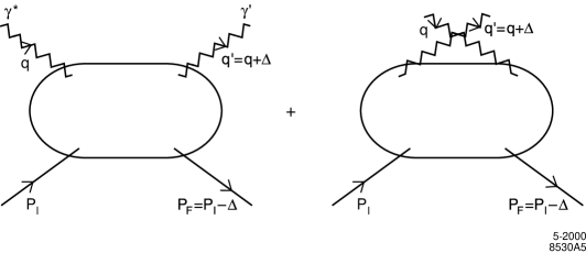
Figure 1: The virtual Compton amplitude $\gamma^{*}(q)+p(P)\to\gamma(q^{\prime})+p(P^{\prime})$.

To leading order in $1/Q$, the deeply virtual Compton scattering amplitude factorizes as the convolution in $x$ of the amplitude for hard Compton scattering on a quark line with skewed parton distributions $H(x,\zeta,t),$ $E(x,\zeta,t)$, $\widetilde{H}(x,\zeta,t),$ and $\widetilde{E}(x,\zeta,t)$ of the target proton. Here $x$ is the light-cone momentum fraction of the struck quark, and $\zeta=Q^{2}/(2P\cdot q)$ plays the role of the Bjorken variable known from deep inelastic scattering. One can also interpret these distributions in terms of virtual quark-proton scattering amplitudes as defined in the covariant parton model [8, 11, 12].

There are remarkable sum rules connecting $H(x,\zeta,t)$ and $E(x,\zeta,t)$ with the corresponding helicity conserving and helicity flip electromagnetic form factors $F_{1}(t)$ and $F_{2}(t)$ and gravitational form factors $A_{q}(t)$ and $B_{q}(t)$ for each quark and anti-quark constituent [2]. For example, the gravitational form factors are given by

$$\int_{0}^{1}{{\rm d}x\over 1-{\zeta\over 2}}\ {x-{\zeta\over 2}\over 1-{\zeta\over 2}}\ [H(x,\zeta,t)+E(x,\zeta,t)]\ =\ A_{q}(t)+B_{q}(t)\ .\\$$

Thus deeply virtual Compton scattering is related to the quark contribution to the form factors of a proton scattering in a gravitational field. The total anomalous gravito-magnetic moment $B(t=0)$ vanishes identically when summed over all constituents [13]. In the present work the close connection between skewed parton distributions and hadronic form factors will become apparent. To emphasize this relationship, we will refer to $H,E,\widetilde{H}$ and $\widetilde{E}$ as “generalized Compton form factors”.

It has long been known that the conventional parton distributions which describe deep inelastic scattering can be represented in terms of the squared light-cone Fock-state wavefunction of the proton target [14]. This representation reflects the fact that parton distributions can be understood as probability densities. In contrast, virtual Compton scattering always involves non-zero momentum transfer, and a probabilistic interpretation of skewed parton distributions is not possible. However, these distributions can still be constructed from specific overlap integrals of the proton wavefunctions. They can in fact be regarded as interference terms between wavefunctions for different parton configurations, containing information on the proton structure that is not accessible at the level of probability densities. This overlap representation is the focus of the present work.

There are three distinct integration regions in $x$. In the domain where $\zeta<x<1$, the generalized form factors $H$, $E$, $\widetilde{H}$ and $\widetilde{E}$ correspond to the situation where one removes a quark from the initial proton wavefunction at light-cone momentum fraction $x=k^{+}/P^{+}$ and transverse momentum ${\vec{k}_{\perp}}$ and re-inserts it into the final-state wavefunction of the proton with the same chirality, but with light-cone momentum fraction $x-\zeta$ and transverse momentum ${\vec{k}_{\perp}}-{\vec{\Delta}_{\perp}}$. The domain $\zeta-1<x<0$ corresponds to removing an antiquark with momentum fraction $\zeta-x$ and re-inserting it with momentum $-x$, both momentum fractions being positive as they must. In the remaining integration domain, $0<x<\zeta$, the photons scatter off of a virtual quark-antiquark pair in the initial proton wavefunction: the quark of the pair has light-cone momentum fraction $x$ and transverse momentum ${\vec{k}_{\perp}}$, whereas the anti-quark has light-cone momentum fraction $\zeta-x$ and transverse momentum ${\vec{\Delta}_{\perp}}-{\vec{k}_{\perp}}$. This domain is unique to skewed parton distributions and does not appear in the usual parton densities, where $\zeta=0$.

In the case of matrix elements of space-like currents, one can choose the special frame $(P-P^{\prime})^{+}=0$, as in the Drell-Yan-West representation of the space-like electromagnetic form factors [15]. Thus given the light-cone wavefunctions, one can construct space-like electromagnetic, electroweak, gravitational couplings, or any local operator product matrix element from their overlap [13, 16]. This overlap is diagonal in parton number. In the case of deeply virtual Compton scattering, the proton matrix elements require the computation of the diagonal, parton number conserving, matrix element $n\rightarrow n$ for the regions $\zeta<x<1$ and $\zeta-1<x<0$ [17]. However, it also involves an off-diagonal $n+1\rightarrow n-1$ convolution for $0<x<\zeta$, where the parton number is decreased by two. This domain occurs since the current operator of the final-state photon with positive light-cone momentum fraction $\zeta$ can annihilate a quark-antiquark pair in the initial proton wavefunction. This type of overlap has first been identified in the context of the form factors which control time-like semi-leptonic $B$ decay [18]. As we shall see, there are underlying relations between Fock states of different particle number which interrelate the two types of overlap.

It also should be noted that the calculation of deep inelastic structure functions and space-like form factors requires the light-cone frame choice $(P-P^{\prime})^{+}\neq 0$ in one-space and one-time theories for $(P-P^{\prime})^{2}\neq 0$. Explicit non-perturbative results for space-like form factors and structure functions of $QCD(1+1)$ with $N_{C}\to\infty$ have been given by Einhorn [19]. The application to deeply virtual Compton scattering in $QCD(1+1)$ has recently been given by Burkardt [20].

In order to illustrate the general formalism for $3+1$ theories, we will present an explicit calculation of deeply virtual Compton scattering on a fermion in quantum electrodynamics at one-loop order. The Feynman amplitudes which are evaluated are shown in Fig. 2. The QED calculation [13, 16] is patterned after the structure which occurs in the one-loop Schwinger ${\alpha/2\pi}$ correction to the electron magnetic moment. In effect, we will represent a spin-$\frac{1}{2}$ system as a composite of a spin-$\frac{1}{2}$ fermion and spin-one vector boson with arbitrary masses. The one-loop model illustrates the interrelations between Fock states of different particle number as required by the boost invariance of space-like form factors or, equivalently, by the $\zeta$ independence of the first moment in $x$ of the generalized Compton form factors $H(x,\zeta,t)$ and $E(x,\zeta,t)$.

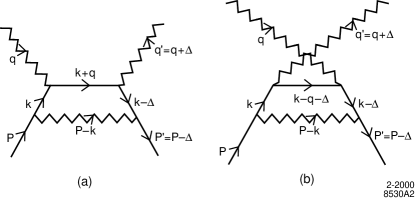
Figure 2: One-loop covariant Feynman diagrams for virtual Compton scattering in QED.

The one-loop model can be further generalized by applying spectral Pauli-Villars integration over the constituent masses. The resulting form of light-cone wavefunctions provides a template for parametrizing the structure of relativistic composite systems and their matrix elements in hadronic physics. For example, this model has recently been used to clarify the connection of parton distributions to the constituents’ spin and orbital angular momentum and to other observables of the composite system such as its electromagnetic and gravitational moments and form factors [13]. The model also provides a self-consistent form for the wavefunctions of an effective quark-diquark model of the valence Fock state of the proton wavefunction.

This paper is organized as follows. After introducing the necessary kinematics in Section 2, we review in Section 3 the representation of deeply virtual Compton scattering in terms of generalized form factors, and the sum rules connecting them with the form factors of the electromagnetic and gravitational currents. In Section 4 we represent the generalized Compton form factors in terms of light-cone wavefunctions, starting from the Fock state representation of a composite system. The following section applies this framework to the explicit cases of QED at one loop. We summarize our results in Section 6. Throughout our paper we shall use momentum variables as employed by Radyushkin [3], which provide an intuitive parametrization in the context of wavefunction overlaps. In the Appendix we give our main formulae in the momentum variables of Ji [2], which make the symmetry between the incoming and outgoing proton more explicit.

2 The Kinematics of Virtual Compton Scattering

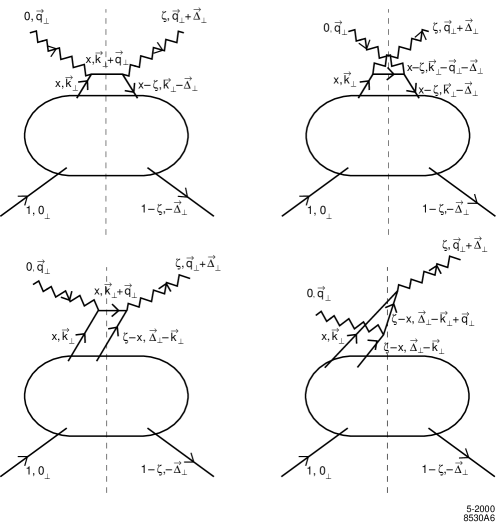
Figure 3: Light-cone time-ordered contributions to deeply virtual Compton scattering. Only the contributions of leading power in $1/Q$ are illustrated. These contributions illustrate the factorization property of the leading twist amplitude.

We begin with the kinematics of virtual Compton scattering

$$\gamma^{*}(q)+p(P)\to\gamma(q^{\prime})+p(P^{\prime})\ ,$$ (1)

see Fig. 3. We specify the frame by choosing a convenient parametrization of the light-cone coordinates for the initial and final proton:

$$P = \left(\ P^{+}\ ,\ {\vec{0}_{\perp}}\ ,\ {M^{2}\over P^{+}}\ \right)\ ,$$ (2)

$$P^{\prime} = \left((1-\zeta)P^{+}\ ,\ -{\vec{\Delta}_{\perp}}\ ,\ {M^{2}+{\vec{\Delta}_{\perp}}^{2}\over(1-\zeta)P^{+}}\right)\ ,$$ (3)

where $M$ is the proton mass. We use the component notation $V=(V^{+},\vec{V}_{\perp},V^{-})$, and our metric is specified by $V^{\pm}=V^{0}\pm V^{z}$ and $V^{2}=V^{+}V^{-}-{\vec{V}}_{\perp}^{2}$. The four-momentum transfer from the target is

$$\Delta = P-P^{\prime}\ =\ \left(\zeta P^{+}\ ,\ {\vec{\Delta}_{\perp}}\ ,\ {t+{\vec{\Delta}_{\perp}}^{2}\over\zeta P^{+}}\right)\ ,$$ (4)

where $t=\Delta^{2}$. In addition, overall energy-momentum conservation requires $\Delta^{-}=P^{-}-P^{\prime-}$, which connects ${\vec{\Delta}_{\perp}}^{2}$, $\zeta$, and $t$ according to

$$t\ =\ 2P\cdot\Delta\ =\ -{\zeta^{2}M^{2}+{\vec{\Delta}_{\perp}}^{2}\over 1-\zeta}\ .$$ (5)

As in the case of space-like form factors, it is convenient to choose a frame where the incident space-like photon carries $q^{+}=0$ so that $q^{2}=-Q^{2}=-{\vec{q}_{\perp}}^{\;2}$:

$$q = \left(0\ ,\ {\vec{q}_{\perp}}\ ,\ {({\vec{q}_{\perp}}+{\vec{\Delta}_{\perp}})^{2}\over\zeta P^{+}}+{\zeta M^{2}+{\vec{\Delta}_{\perp}}^{2}\over(1-\zeta)P^{+}}\right)\ ,$$ (6)

$$q^{\prime} = \left(\zeta P^{+}\ ,\ {\vec{q}_{\perp}}+{\vec{\Delta}_{\perp}}\ ,\ {({\vec{q}_{\perp}}+{\vec{\Delta}_{\perp}})^{2}\over\zeta P^{+}}\right)\ .$$ (7)

Thus no light-cone time-ordered amplitudes involving the splitting of the incident photon can occur. The variable $\zeta$ is fixed from (2) and (6) as

$$2P\cdot q={({\vec{q}_{\perp}}+{\vec{\Delta}_{\perp}})^{2}\over\zeta}+{\zeta M^{2}+{\vec{\Delta}_{\perp}}^{2}\over 1-\zeta}\ .$$ (8)

We will be interested in deeply virtual Compton scattering, where $Q^{2}$ is large compared to the masses and $-t$. Then, we have

$${Q^{2}\over 2P\cdot q}=\zeta\$$ (9)

up to corrections in $1/Q^{2}$. Thus $\zeta$ plays the role of the Bjorken variable in deeply virtual Compton scattering. For a fixed value of $-t$, the allowed range of $\zeta$ is given by

$$0\ \leq\ \zeta\ \leq\ {(-t)\over 2M^{2}}\ \ \left({\sqrt{1+{4M^{2}\over(-t)}}}\ -\ 1\ \right)\ .$$ (10)

The choice of parametrization of the light-cone frame is of course arbitrary. For example, in the Appendix, we show how one can conveniently utilize a “symmetric” frame for the incoming and outgoing proton, which has manifest symmetry under crossing $P\leftrightarrow P^{\prime}$.

3 The Generalized Form Factors of Deeply Virtual Compton Scattering

The virtual Compton amplitude $M^{\mu\nu}({\vec{q}_{\perp}},{\vec{\Delta}_{\perp}},\zeta)$, i.e., the transition matrix element of the process $\gamma^{*}(q)+p(P)\to\gamma(q^{\prime})+p(P^{\prime})$, can be defined from the light-cone time-ordered product of currents

$$M^{\mu\nu}({\vec{q}_{\perp}},{\vec{\Delta}_{\perp}},\zeta)\ =\ i\int d^{4}y\,e^{-iq\cdot y}\langle P^{\prime}|TJ^{\mu}(y)J^{\nu}(0)|P\rangle\ ,$$ (11)

where the Lorentz indices $\mu$ and $\nu$ denote the polarizations of the initial and final photons respectively. An essential characteristic of deeply virtual Compton scattering in light-cone gauge is that any soft interaction with the target which occurs between the light-cone times of the incident and final photon is power-law suppressed as $1/Q$. Similarly, the diagrams in which the photons hit two different quark lines in the target are also higher twist. We can then replace the fully interacting currents $J^{\mu}(y)$ and $J^{\nu}(0)$ by the quark currents $j^{\mu}(y)$ and $j^{\nu}(0)$ of the non-interacting theory, which have simple matrix elements in the free Fock basis. The leading contribution thus factorizes as a hard-scattering amplitude involving the elementary photon interactions on a quark line convoluted with the non-perturbative light-cone wavefunctions of the protons, see Fig. 3. In the limit $Q^{2}\to\infty$ at fixed $\zeta$ and $t$ the Compton amplitude is thus given by

$$M^{IJ}({\vec{q}_{\perp}},{\vec{\Delta}_{\perp}},\zeta)\ =\ \epsilon^{I}_{\mu}\,\epsilon^{*J}_{\nu}\,M^{\mu\nu}({\vec{q}_{\perp}},{\vec{\Delta}_{\perp}},\zeta)\ =\ -e^{2}_{q}\ {1\over 2\bar{P}^{+}}\int_{\zeta-1}^{1}{\rm d}x\$$

$$\times \left\{\ {t}^{IJ}(x,\zeta)\ {\bar{U}}(P^{\prime})\left[H(x,\zeta,t)\ {\gamma^{+}}+E(x,\zeta,t)\ {i\over 2M}\,{\sigma^{+\alpha}}(-\Delta_{\alpha})\right]U(P)\right.$$

$$\ \ \left.{s}^{IJ}(x,\zeta)\ {\bar{U}}(P^{\prime})\left[{\widetilde{H}}(x,\zeta,t)\ {\gamma^{+}\gamma_{5}}+{\widetilde{E}}(x,\zeta,t)\ {1\over 2M}\,{\gamma_{5}}(-\Delta^{+})\right]U(P)\ \right\},$$

where $\bar{P}={1\over 2}(P^{\prime}+P)$. In getting (3) we used the relations $\gamma^{1}\gamma^{+}\gamma^{1}=\gamma^{2}\gamma^{+}\gamma^{2}=\gamma^{+}$ and $\gamma^{1}\gamma^{+}\gamma^{2}=-\gamma^{2}\gamma^{+}\gamma^{1}=i\gamma^{+}\gamma_{5}$. For simplicity we only consider one quark with flavor $q$ and electric charge $e_{q}$ here and in the sequel. Throughout our analysis we will use the Born approximation to the photon-quark amplitude. The radiative QCD corrections to this process have been calculated to order $\alpha_{s}$ in [6, 21].

For circularly polarized initial and final photons ($I,\ J$ are $\uparrow$ or $\downarrow)$) we have

$${t}^{\ \uparrow\uparrow}(x,\zeta) = \phantom{-}\ {t}^{\ \downarrow\downarrow}(x,\zeta)\ =\ {1\over x-i\epsilon}\ +\ {1\over x-\zeta+i\epsilon}\ ,$$ (13)

$${s}^{\ \uparrow\uparrow}(x,\zeta) = -\ {s}^{\ \downarrow\downarrow}(x,\zeta)\ =\ {1\over x-i\epsilon}\ -\ {1\over x-\zeta+i\epsilon}\ ,$$

$${t}^{\ \uparrow\downarrow}(x,\zeta) = {t}^{\ \downarrow\uparrow}(x,\zeta)\ =\ {s}^{\ \uparrow\downarrow}(x,\zeta)\ =\ {s}^{\ \downarrow\uparrow}(x,\zeta)\ \ =\ \ 0\ \phantom{\frac{1}{2}}.$$

The two photon polarization vectors in light-cone gauge are given by

$$\epsilon^{\uparrow,\downarrow}=\left(0\ ,\ \vec{\epsilon}^{\ \uparrow,\downarrow}_{\perp}\ ,\ {\vec{\epsilon}^{\ \uparrow,\downarrow}_{\perp}\cdot\vec{k}_{\perp}\over 2k^{+}}\right)\ ,\qquad\vec{\epsilon}_{\perp}^{\ \uparrow,\downarrow}=\mp{1\over\sqrt{2}}\left(\begin{array}[]{c}1\\ \pm i\end{array}\right)\ ,$$ (14)

where $k$ denotes the appropriate photon momentum. The polarization vectors satisfy the Lorentz condition $k\cdot\epsilon=0$. For a longitudinally polarized initial photon, the Compton amplitude is of order $1/Q$ and thus vanishes in the limit $Q^{2}\to\infty$. At order $1/Q$ there are several corrections to the simple structure in Eq. (3). Those corrections which correspond to the evaluation of the diagrams in Fig. 3 to accuracy $1/Q$ can be described by functions related to the form factors $H$, $E$ or ${\widetilde{H}}$, ${\widetilde{E}}$ through Wandzura-Wilczek type integral relations. In other contributions the hard scattering is no longer on a single quark line, so that new non-perturbative functions appear. For details we refer to [5, 22].

In (3) the generalized form factors $H$, $E$ and ${\widetilde{H}}$, ${\widetilde{E}}$ are defined through matrix elements of the bilinear vector and axial vector currents on the light-cone:

$$\int\frac{dy^{-}}{8\pi}\;e^{ixP^{+}y^{-}/2}\;\langle P^{\prime}|\bar{\psi}(0)\,\gamma^{+}\,\psi(y)\,|P\rangle\Big{|}_{y^{+}=0,y_{\perp}=0}$$

$$= {1\over 2\bar{P}^{+}}\ {\bar{U}}(P^{\prime})\left[\,H(x,\zeta,t)\ {\gamma^{+}}+E(x,\zeta,t)\ {i\over 2M}\,{\sigma^{+\alpha}}(-\Delta_{\alpha})\right]U(P)\ ,$$

$$\int\frac{dy^{-}}{8\pi}\;e^{ixP^{+}y^{-}/2}\;\langle P^{\prime}|\bar{\psi}(0)\,\gamma^{+}\gamma_{5}\,\psi(y)\,|P\rangle\Big{|}_{y^{+}=0,y_{\perp}=0}$$

$$= {1\over 2\bar{P}^{+}}\ {\bar{U}}(P^{\prime})\left[\,{\widetilde{H}}(x,\zeta,t)\ {\gamma^{+}\gamma_{5}}+{\widetilde{E}}(x,\zeta,t)\ {1\over 2M}\,{\gamma_{5}}(-\Delta^{+})\,\right]U(P)\ .$$

We can compare these generalized form factors for the Compton amplitude with the matrix elements of the electromagnetic and gravitational currents. For the electromagnetic current $e_{q}J^{\mu}(y)=e_{q}{\bar{\psi}}(y)\gamma^{\mu}\psi(y)$, one has the usual Dirac and Pauli form factors

$$\langle P^{\prime}|J^{\mu}(0)|P\rangle=\bar{U}(P^{\prime})\left[\,F_{1}(t)\,\gamma^{\mu}+F_{2}(t)\,{i\over 2M}\,\sigma^{\mu\alpha}(-\Delta_{\alpha})\,\right]U(P)\ ,$$ (16)

where for later convenience we have not included the charge $e_{q}$ in the definitions of the current and the form factors. For the form factors of the energy-momentum tensor for a spin-${1\over 2}$ composite system, one defines [2, 23]

$$\langle P^{\prime}|T^{\mu\nu}(0)|P\rangle = \bar{U}(P^{\prime})\left[\,A_{q}(t)\,{\gamma}^{(\mu}\,\bar{P}^{\nu)}+B_{q}(t)\,{i\over 2M}\bar{P}^{(\mu}{\sigma}^{\nu)\alpha}(-\Delta_{\alpha})\right.$$ (17)

$$\qquad\qquad+\left.C_{q}(t)\,{1\over M}\,(\Delta^{\mu}\Delta^{\nu}-g^{\mu\nu}\Delta^{2})\,\right]U(P)\ ,$$

where $a^{(\mu}b^{\nu)}={1\over 2}(a^{\mu}b^{\nu}+a^{\nu}b^{\mu})$ and

$$T^{\mu\nu}={i\over 4}\ \Big{(}\ {\bar{\psi}}\gamma^{\mu}\overrightarrow{\partial}{}^{\nu}\psi-{\bar{\psi}}\gamma^{\mu}\overleftarrow{\partial}{}^{\nu}\psi\ \Big{)}\ +\ \{\ \mu\longleftrightarrow\nu\ \}\$$ (18)

is the quark part of the energy-momentum tensor. These form factors can be computed in a form similar to that of the virtual Compton amplitude if we choose the light-cone frame where the virtual photon or graviton has momentum $q^{+}=\zeta P^{+}$ and ${\vec{q}_{\perp}}={\vec{\Delta}_{\perp}}$. In the electromagnetic case, the coupling of the current $e_{q}J^{+}(0)$ on the quark line is identical to the Compton amplitude with $e_{q}^{2}\,t^{IJ}$ replaced simply by the quark charge $e_{q}$. One finds

$$\int_{\zeta-1}^{1}{{\rm d}x\over 1-{\zeta\over 2}}\ H(x,\zeta,t) = F_{1}(t)\ ,$$ (19)

$$\int_{\zeta-1}^{1}{{\rm d}x\over 1-{\zeta\over 2}}\ E(x,\zeta,t) = F_{2}(t)\ ,$$

Analogous sum rules relate $\widetilde{H}$ and $\widetilde{E}$ with the form factors of the axial vector current $J_{5}^{\mu}(y)={\bar{\psi}}(y)\gamma^{\mu}\gamma_{5}\psi(y)$. The factors $1-\zeta/2$ in (19) appear because we use Ji’s normalization convention for the Compton form factors, which involves $\bar{P}^{+}$ on the right-hand side of (3), and at the same time parametrize light-cone momentum fractions with respect to $P^{+}=(1-\zeta/2)\bar{P}^{+}$. In the Appendix we will give our main formulae in the parametrization of Ji, where momentum fractions refer to $\bar{P}^{+}$.

In the case of the gravitational form factors, the derivative coupling in the graviton current $T^{++}$ brings in an extra factor $x-\zeta/2$. Then, one gets the sum rule [2]

$$\int_{\zeta-1}^{1}{{\rm d}x\over 1-{\zeta\over 2}}\ {x-{\zeta\over 2}\over 1-{\zeta\over 2}}\ [H(x,\zeta,t)+E(x,\zeta,t)]\ =\ A_{q}(t)\ +\ B_{q}(t)\ .$$ (20)

The gravitational form factor $C_{q}(t)$ cancels for the combination $H+E$, as we shall show shortly.

When we take the $\mu=+$ component in (16), the factors of the two terms in the right hand side are given by

$${1\over 2\bar{P}^{+}}\ {\bar{U}}(P^{\prime},{\lambda}^{\prime}){\gamma^{+}}\,U(P,\lambda) = {\sqrt{1-\zeta}\over 1-{\zeta\over 2}}\ \delta_{\lambda,\,{\lambda}^{\prime}}\ ,$$ (21)

$${1\over 2\bar{P}^{+}}\ {\bar{U}}(P^{\prime},{\lambda}^{\prime}){i\over 2M}\,{\sigma^{+\alpha}}(-\Delta_{\alpha})U(P,\lambda) = -\,{\zeta^{2}\over 4{(1-{\zeta\over 2})\sqrt{1-\zeta}}}\ \delta_{\lambda,\,{\lambda}^{\prime}}$$

$$+\ {1\over\sqrt{1-\zeta}}\;{\,-\lambda\Delta^{1}\,-\,i\Delta^{2}\,\over 2M}\ \delta_{\lambda,\,-{\lambda}^{\prime}}\ ,$$

where $\lambda=\pm 1$ is the light-cone helicity of the initial fermion. Then, in the light-cone formalism, the Dirac and Pauli form factors can be identified from the helicity-conserving and helicity-flip vector current matrix elements:

$$\left\langle{P^{\prime},\uparrow\left|\frac{J^{+}(0)}{2\bar{P}^{+}}\right|P,\uparrow}\right\rangle = {\sqrt{1-\zeta}\over 1-{\zeta\over 2}}\,F_{1}(t)\,-\,{\zeta^{2}\over 4(1-{\zeta\over 2}){\sqrt{1-\zeta}}}\,F_{2}(t)\ ,$$ (22)

$$\left\langle{P^{\prime},\uparrow\left|\frac{J^{+}(0)}{2\bar{P}^{+}}\right|P,\downarrow}\right\rangle = {1\over\sqrt{1-\zeta}}\;{\Delta^{1}-{i}\Delta^{2}\over 2M}\,F_{2}(t)\ .$$ (23)

For the matrix element (17) of the energy-momentum tensor we also need

$${1\over 2M}\ {\bar{U}}(P^{\prime},{\lambda}^{\prime})U(P,\lambda)\ =\ {1-{\zeta\over 2}\over{\sqrt{1-\zeta}}}\ \delta_{\lambda,\,{\lambda}^{\prime}}-{1\over{\sqrt{1-\zeta}}}\;{-\lambda\Delta^{1}\,-\,i\Delta^{2}\over 2M}\ \delta_{\lambda,\,-{\lambda}^{\prime}}\ .$$ (24)

One easily checks that (21) and (24) satisfy the Gordon identity. With this we have

$$\left\langle{P^{\prime},\uparrow\left|\frac{T^{++}(0)}{2(\bar{P}^{+})^{2}}\right|P,\uparrow}\right\rangle = {\sqrt{1-\zeta}\over 1-{\zeta\over 2}}\,A_{q}(t)\,-\,{\zeta^{2}\over 4(1-{\zeta\over 2}){\sqrt{1-\zeta}}}\,B_{q}(t)$$ (25)

$$+\ {\zeta^{2}\over(1-{\zeta\over 2}){\sqrt{1-\zeta}}}\,C_{q}(t)\ ,$$

$$\left\langle{P^{\prime},\uparrow\left|\frac{T^{++}(0)}{2(\bar{P}^{+})^{2}}\right|P,\downarrow}\right\rangle = \left\{{1\over{\sqrt{1-\zeta}}}\,B_{q}(t)\right.$$ (26)

$$\left.-\ {\zeta^{2}\over(1-{\zeta\over 2})^{2}{\sqrt{1-\zeta}}}\,C_{q}(t)\ \right\}\ {\Delta^{1}-{i}\Delta^{2}\over 2M}\ .$$

Combining (25) and (26), we get

$${1\over 1-{\zeta\over 2}}\left\langle{P^{\prime},\uparrow\left|\frac{T^{++}(0)}{2(\bar{P}^{+})^{2}}\right|P,\uparrow}\right\rangle+{2M\over{\Delta^{1}-{i}\Delta^{2}}}\left\langle{P^{\prime},\uparrow\left|\frac{T^{++}(0)}{2(\bar{P}^{+})^{2}}\right|P,\downarrow}\right\rangle$$

$$={\sqrt{1-\zeta}\over(1-{\zeta\over 2})^{2}}\ \left[A_{q}(t)\ +\ B_{q}(t)\right]\ ,$$ (27)

whereas from (22) and (23) we have

$${1\over 1-{\zeta\over 2}}\left\langle{P^{\prime},\uparrow\left|\frac{J^{+}(0)}{2\bar{P}^{+}}\right|P,\uparrow}\right\rangle+{2M\over{\Delta^{1}-{i}\Delta^{2}}}\left\langle{P^{\prime},\uparrow\left|\frac{J+(0)}{2\bar{P}^{+}}\right|P,\downarrow}\right\rangle$$

$$=\ {\sqrt{1-\zeta}\over(1-{\zeta\over 2})^{2}}\ \left[F_{1}(t)\ +\ F_{2}(t)\right]\ .$$ (28)

Using that $H$ and $E$ involve the same proton helicity structure as $F_{1}$ and $F_{2}$, see (3) and (16), one obtains Ji’s sum rule (20) from the connection between $T^{++}(0)$ and the non-local current defining $H$ and $E$.

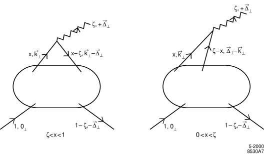
Figure 4: Light-cone time-ordered contributions to spacelike form factors. The sum of the two contributions is $\zeta$-independent at fixed $t=\Delta^{2}$.

In (19) we can separate three distinct regions of integration:

$$(1-\zeta/2)\,F_{1}(t)\rule[-8.61108pt]{0.0pt}{8.61108pt}$$

$$= \int_{\zeta-1}^{0}{\rm d}x\ H_{(n\to n)}(x,\zeta,t)+\int_{0}^{\zeta}{\rm d}x\ H_{(n+1\to n-1)}(x,\zeta,t)+\int_{\zeta}^{1}{\rm d}x\ H_{(n\to n)}(x,\zeta,t)\,$$

where

$$H(x,\zeta,t) = H_{(n\to n)}(x,\zeta,t)\ [\theta(x-\zeta)+\theta(-x)]$$

$$+ H_{(n+1\to n-1)}(x,\zeta,t)\ \theta(\zeta-x)\,\theta(x)\ .$$

Similarly,

$$(1-\zeta/2)\,F_{2}(t)\rule[-8.61108pt]{0.0pt}{8.61108pt}$$

$$= \int_{\zeta-1}^{0}{\rm d}x\ E_{(n\to n)}(x,\zeta,t)+\int_{0}^{\zeta}{\rm d}x\ E_{(n+1\to n-1)}(x,\zeta,t)+\int_{\zeta}^{1}{\rm d}x\ E_{(n\to n)}(x,\zeta,t)\,$$

with

$$E(x,\zeta,t) = E_{(n\to n)}(x,\zeta,t)\ [\theta(x-\zeta)+\theta(-x)]$$

$$+ E_{(n+1\to n-1)}(x,\zeta,t)\ \theta(\zeta-x)\,\theta(x)\ .$$

From the point of view of the form factors $F_{1}(t)$ and $F_{2}(t)$, the division of the $x$-integrals into separate domains $\zeta-1<x<0$, $0<x<\zeta$, and $\zeta<x<1$ is an artifact of the light-cone frame choice. The two types of contributions to space-like form factors are illustrated in Fig. 4. In the region $\zeta<x<1$ a quark is scattered off the current, whereas the region $\zeta-1<x<0$ corresponds to scattering of an antiquark. For $0<x<\zeta$, however, the current annihilates a quark-antiquark pair in the target.

The $x$-integrals of $(1-\zeta/2)^{-1}\,H(x,\zeta,t)$ and $(1-\zeta/2)^{-1}\,E(x,\zeta,t)$ are independent of $\zeta$ as a consequence of Lorentz invariance. Thus, the contributions of the $n$, $n-1$, and $n+1$ particle light-cone wavefunctions are in fact not independent. This deeply reflects the underlying frame invariance of the light-cone Fock representation [24], which ensures the independence of the form factors from the frame choice for the graviton or photon momentum $\Delta^{+}=\zeta P^{+}$ as long as $\Delta^{2}=t$ is kept fixed.

To see how this occurs in a simple example, we shall consider the matrix element for the scattering of two scalar particles, $k+(P-k)\to\Delta+(P-\Delta)$, in $\phi^{3}$ theory. In order to make the result resemble the integrand of a form factor, we parametrize $k^{+}=xP^{+}$ and $\Delta^{+}=\zeta P^{+}$. The particle with momentum $\Delta$ represents the external current, whereas the other external particles are on their mass shell, $k^{2}=(P-k)^{2}=(P-\Delta)^{2}=m^{2}$. Four-momentum conservation implies $k^{-}+(P-k)^{-}=\Delta^{-}+(P-\Delta)^{-}$. The Born amplitude from exchanging a scalar particle with momentum $\Delta-k$ in the $t$-channel receives two time-ordered contributions in light-cone perturbation theory, see Fig. 5:

$${\cal M}_{k+(P-k)\to\Delta+(P-\Delta)} = {g^{2}\theta(\zeta-x)\over(\Delta-k)^{+}\left[(P-k)^{-}-(P-\Delta)^{-}-{(\vec{\Delta}_{\perp}-\vec{k}_{\perp})^{2}+m^{2}\over(\Delta-k)^{+}}+i\epsilon\right]}\ \ \$$

$$+ {g^{2}\theta(x-\zeta)\over(k-\Delta)^{+}\left[k^{-}-\Delta^{-}-{(\vec{k}_{\perp}-\vec{\Delta}_{\perp})^{2}+m^{2}\over(k-\Delta)^{+}}+i\epsilon\right]}\ .$$

Since the particle with momentum $\Delta$ represents the external current we have treated it as an on-shell particle with mass squared $\Delta^{2}$, so that $\Delta^{-}=(\vec{\Delta}_{\perp}^{2}+\Delta^{2})/\Delta^{+}$ appears in the energy denominator of the second term [14]. Then, the sum of the light-cone contributions must agree with the covariant result

$${\cal M}_{k+(P-k)\to\Delta+(P-\Delta)}\ =\ {g^{2}\over(k-\Delta)^{2}-m^{2}+i\epsilon}\,$$ (34)

independent of $\zeta$. In fact, replacing $(P-k)^{-}-(P-\Delta)^{-}$ with $\Delta^{-}-k^{-}$ in the first term, we see that the identity is trivial since the two denominators in ${\cal M}$ are identical, differing only in whether $0<x<\zeta$ or $\zeta<x<1$ as determined by the arbitrary choice of frame.

Figure 5: Light-cone time-ordered contributions from $t$-channel exchange in the scattering process $k+(P-k)\to\Delta+(P-\Delta)$ in $\phi^{3}$ theory.

The scattering amplitude can also be interpreted as a simple model for a scalar current form factor $\left\langle{P-\Delta|J(0)|P}\right\rangle.$ In this model, one interprets the initial state $|P\rangle$ as a wave packet of the incident particles with momenta $P-k$ and $k$. The particle with momentum $\Delta$ represents again the particle coupling to the current. The two light-cone time-ordered contributions of $\cal M$ correspond to the $3\to 1$ and $2\to 2$ light-cone wavefunction overlap contributions to the form factor, respectively. Thus in this simple model, the division of contributions from the $3\to 1$ and $2\to 2$ light-cone wavefunctions corresponds simply to the partition of a common $x$ integrand into regions $0<x<\zeta$ and $\zeta<x<1$.

4 The Light-Cone Fock Representation of Deeply Virtual Compton Scattering

The light-cone Fock expansion of hadrons is constructed by quantizing QCD at fixed light-cone time $\tau=t+z/c$ and forming the invariant light-cone Hamiltonian: $H_{LC}=P^{+}P^{-}-{\vec{P}_{\perp}}^{2}$, see [25]. While the momentum generators $P^{+}$ and $\vec{P}_{\perp}$ are kinematical, i.e., they are independent of the interactions, the generator $P^{-}=i{{\mathrm{d}}\over{\mathrm{d}}\tau}$ generates light-cone time translation. The eigen-spectrum of $H_{LC}$ gives the entire mass spectrum of the color-singlet hadron states in QCD, together with their respective light-cone wavefunctions. In particular, the proton state satisfies $H_{LC}|\,{\psi_{p}}\rangle=M^{2}|\,{\psi_{p}}\rangle$. Such equations can be solved in principle using the discretized light-cone quantization (DLCQ) method [26]. The expansion of the proton eigensolution $|\,{\psi_{p}}\rangle$ on the eigenstates $\{|\,{n}\rangle\}$ of the free Hamiltonian $H_{LC}(g=0)$ gives the light-cone Fock expansion:

$$\left|\psi_{p}(P^{+},{\vec{P}_{\perp}})\right> = \sum_{n}\ \prod_{i=1}^{n}{{\rm d}x_{i}\,{\rm d}^{2}{\vec{k}_{\perp i}}\over\sqrt{x_{i}}\,16\pi^{3}}\ \,16\pi^{3}\delta\left(1-\sum_{i=1}^{n}x_{i}\right)\,\delta^{(2)}\left(\sum_{i=1}^{n}{\vec{k}_{\perp i}}\right)$$

$$\qquad\rule{0.0pt}{19.37494pt}\times\psi_{n}(x_{i},{\vec{k}_{\perp i}},\lambda_{i})\left|n;\,x_{i}P^{+},x_{i}{\vec{P}_{\perp}}+{\vec{k}_{\perp i}},\lambda_{i}\right>.$$

The light-cone momentum fractions $x_{i}=k^{+}_{i}/P^{+}$ and ${\vec{k}_{\perp i}}$ represent the relative momentum coordinates of the QCD constituents. The physical transverse momenta are ${\vec{p}_{\perp i}}=x_{i}{\vec{P}_{\perp}}+{\vec{k}_{\perp i}}.$ The $\lambda_{i}$ label the light-cone spin projections $S^{z}$ of the quarks and gluons along the quantization direction $z$. The $n$-particle states are normalized as

$$\left<n;\,p^{\prime}_{i}{}^{+},{\vec{p}\,^{\prime}_{\perp i}},\lambda^{\prime}_{i}\right.\,\left|n;\,p^{~{}}_{i}{}^{\!\!+},{\vec{p}^{~{}}_{\perp i}},\lambda_{i}\right>=\prod_{i=1}^{n}16\pi^{3}p_{i}^{+}\delta(p^{\prime}_{i}{}^{+}-p^{~{}}_{i}{}^{\!\!+})\ \delta^{(2)}({\vec{p}\,^{\prime}_{\perp i}}-{\vec{p}^{~{}}_{\perp i}})\ \delta_{\lambda^{\prime}_{i}\lambda^{~{}}_{i}}\ .$$ (36)

Here and in the following we will not display the other quantum numbers of the partons, i.e., color and quark flavor. We will also not discuss the case where a Fock state contains partons with identical helicity, flavor, and color. For a discussion of these points we refer to [27].

The solutions of $H_{LC}|\,{\psi_{p}}\rangle=M^{2}|\,{\psi_{p}}\rangle$ are independent of $P^{+}$ and ${\vec{P}_{\perp}}$; thus given the eigensolution Fock projections $\langle n;\ x_{i},{\vec{k}_{\perp i}},\lambda_{i}|\psi_{p}\rangle\propto\psi_{n}(x_{i},{\vec{k}_{\perp i}},\lambda_{i})$, the wavefunction of the proton is determined in any frame [14]. The light-cone wavefunctions $\psi_{n}(x_{i},\vec{k}_{\perp i},\lambda_{i})$ encode all of the bound state quark and gluon properties of hadrons, including their momentum, spin and flavor correlations, in the form of universal process- and frame-independent amplitudes.

The deeply virtual Compton amplitude can be evaluated explicitly by starting from the Fock state representation for both the incoming and outgoing proton, using the boost properties of the light-cone wavefunctions, and evaluating the matrix elements of the currents for a quark target. One can also directly evaluate the non-local current matrix elements (3) in the same framework. In the following we will concentrate on the generalized Compton form factors $H$ and $E$. Formulae analogous to our results can be obtained for $\widetilde{H}$ and $\widetilde{E}$.

For the $n\to n$ diagonal term ($\Delta n=0$), the relevant current matrix element at quark level is

$$\int\frac{dy^{-}}{8\pi}\;e^{ixP^{+}y^{-}/2}\;\left<1;\,x^{\prime}_{1}P\,^{\prime+},{\vec{p}\,^{\prime}_{\perp 1},\lambda^{\prime}_{1}}\left|\bar{\psi}(0)\,{\gamma^{+}}\,\psi(y)\,\right|1;\,x^{~{}}_{1}P^{+},{\vec{p}^{~{}}_{\perp 1}},\lambda^{~{}}_{1}\right>\Big{|}_{y^{+}=0,y_{\perp}=0}$$

$$= \sqrt{x^{~{}}_{1}x^{\prime}_{1}}\,\sqrt{1-\zeta}\ \delta(x-x_{1})\ \delta_{\lambda^{\prime}_{1}\lambda^{~{}}_{1}}\ ,$$

where for definiteness we have labeled the struck quark with the index $i=1$. We thus obtain formulae for the diagonal (parton-number-conserving) contributions to $H$ and $E$ in the domain $\zeta\leq x\leq 1$ [17]:

$${\sqrt{1-\zeta}\over 1-{\zeta\over 2}}\,H_{(n\to n)}(x,\zeta,t)\,-\,{\zeta^{2}\over 4(1-{\zeta\over 2}){\sqrt{1-\zeta}}}\,E_{(n\to n)}(x,\zeta,t)$$

$$= {\sqrt{1-\zeta}^{\,2-n}}\,\sum_{n,\lambda_{i}}\int\prod_{i=1}^{n}{{\rm d}x_{i}\,{\rm d}^{2}{\vec{k}}_{\perp i}\over 16\pi^{3}}\ \,16\pi^{3}\delta\left(1-\sum_{j=1}^{n}x_{j}\right)\,\delta^{(2)}\left(\sum_{j=1}^{n}{\vec{k}}_{\perp j}\right)$$

$$\qquad\qquad\rule{0.0pt}{12.91663pt}{}\times\delta(x-x_{1})\ \psi^{\uparrow\ *}_{(n)}(x^{\prime}_{i},{\vec{k}}^{\prime}_{\perp i},\lambda_{i})\ \psi^{\uparrow}_{(n)}(x_{i},{\vec{k}}_{\perp i},\lambda_{i})\ ,$$

$${1\over\sqrt{1-\zeta}}\;{\Delta^{1}-{i}\Delta^{2}\over 2M}\,E_{(n\to n)}(x,\zeta,t)\rule{0.0pt}{19.37494pt}$$

$$= {\sqrt{1-\zeta}^{\,2-n}}\,\sum_{n,\lambda_{i}}\int\prod_{i=1}^{n}{{\rm d}x_{i}\,{\rm d}^{2}{\vec{k}}_{\perp i}\over 16\pi^{3}}\ \,16\pi^{3}\delta\left(1-\sum_{j=1}^{n}x_{j}\right)\,\delta^{(2)}\left(\sum_{j=1}^{n}{\vec{k}}_{\perp j}\right)$$

$$\qquad\qquad\rule{0.0pt}{12.91663pt}{}\times\delta(x-x_{1})\ \psi^{\uparrow\ *}_{(n)}(x^{\prime}_{i},{\vec{k}}^{\prime}_{\perp i},\lambda_{i})\ \psi^{\downarrow}_{(n)}(x_{i},{\vec{k}}_{\perp i},\lambda_{i})\ ,$$

where the arguments of the final-state wavefunction are given by

$$\begin{array}[t]{lll}x^{\prime}_{1}={\displaystyle\frac{x_{1}-\zeta}{1-\zeta}}\,,&{\vec{k}}^{\prime}_{\perp 1}={\vec{k}}^{~{}}_{\perp 1}-{\displaystyle\frac{1-x_{1}}{1-\zeta}}\,{\vec{\Delta}}_{\perp}&\mbox{for the struck quark,}\\[8.61108pt] x^{\prime}_{i}={\displaystyle\frac{x_{i}}{1-\zeta}}\,,&{\vec{k}}^{\prime}_{\perp i}={\vec{k}}^{~{}}_{\perp i}+{\displaystyle\frac{x_{i}}{1-\zeta}}\,{\vec{\Delta}}_{\perp}&\mbox{for the spectators $i=2,\cdots,n$.}\end{array}$$ (40)

One easily checks that $\sum_{i=1}^{n}x^{\prime}_{i}=1$ and $\sum_{i=1}^{n}{\vec{k}}^{\prime}_{\perp i}={\vec{0}}_{\perp}$. In Eqs. (4) and (4) one has to sum over all possible combinations of helicities $\lambda^{~{}}_{i}$ and over all parton numbers $n$ in the Fock states. We also imply a sum over all possible ways of numbering the partons in the $n$-particle Fock state so that the struck quark has the index $i=1$.

Analogous formulae hold in the domain $\zeta-1<x<0$, where the struck parton in the target is an antiquark instead of a quark. Some care has to be taken regarding overall signs arising because fermion fields anticommute. For details we refer to [17, 27].

For the $n+1\to n-1$ off-diagonal term ($\Delta n=-2$), let us consider the case where quark $1$ and antiquark $n+1$ of the initial wavefunction annihilate into the current leaving $n-1$ spectators. Then $x_{n+1}=\zeta-x_{1}$ and ${\vec{k}}_{\perp n+1}={\vec{\Delta}}_{\perp}-{\vec{k}}_{\perp 1}$. The remaining $n-1$ partons have total plus-momentum $(1-\zeta)P^{+}$ and transverse momentum $-{\vec{\Delta}}_{\perp}$. The current matrix element now is

$$\int\frac{dy^{-}}{8\pi}\;e^{ixP^{+}y^{-}/2}\;\left<0\left|\bar{\psi}(0)\,{\gamma^{+}}\,\psi(y)\,\right|2;\ x^{~{}}_{1}P^{+},x^{~{}}_{n+1}P^{+},\;{\vec{p}^{~{}}_{\perp 1}},{\vec{p}^{~{}}_{\perp n+1}},\;\lambda^{~{}}_{1},\lambda^{~{}}_{n+1}\right>\Big{|}_{y^{+}=0,y_{\perp}=0}$$

$$= \sqrt{x_{1}x_{n+1}\phantom{1}\!\!}\,\delta(x-x_{1})\ \delta_{\lambda_{1}\,-\lambda_{n+1}}\ ,$$

and we thus obtain the formulae for the off-diagonal contributions to $H$ and $E$ in the domain $0\leq x\leq\zeta$:

$${\sqrt{1-\zeta}\over 1-{\zeta\over 2}}\,H_{(n+1\to n-1)}(x,\zeta,t)\,-\,{\zeta^{2}\over 4(1-{\zeta\over 2}){\sqrt{1-\zeta}}}\,E_{(n+1\to n-1)}(x,\zeta,t)$$

$$= {\sqrt{1-\zeta}^{\,3-n}}\,\sum_{n,\lambda_{i}}\int\prod_{i=1}^{n+1}{{\rm d}x_{i}\,{\rm d}^{2}{\vec{k}}_{\perp i}\over 16\pi^{3}}\ 16\pi^{3}\delta\left(1-\sum_{j=1}^{n+1}x_{j}\right)\,\delta^{(2)}\left(\sum_{j=1}^{n+1}{\vec{k}}_{\perp j}\right)$$

$$\qquad\qquad\rule{0.0pt}{12.91663pt}{}\times 16\pi^{3}\delta(x_{n+1}+x_{1}-\zeta)\,\delta^{(2)}\left({\vec{k}}_{\perp n+1}+{\vec{k}}_{\perp 1}-{\vec{\Delta}}_{\perp}\right)$$

$$\qquad\qquad\rule{0.0pt}{12.91663pt}{}\times\delta(x-x_{1})\ \psi^{\uparrow\ *}_{(n-1)}(x^{\prime}_{i},{\vec{k}}^{\prime}_{\perp i},\lambda^{~{}}_{i})\ \psi^{\uparrow}_{(n+1)}(x_{i},{\vec{k}}_{\perp i},\lambda_{i})\ \delta_{\lambda_{1}\,-\lambda_{n+1}}\ ,$$

$${1\over\sqrt{1-\zeta}}\;{\Delta^{1}-{i}\Delta^{2}\over 2M}\,E_{(n+1\to n-1)}(x,\zeta,t)\rule{0.0pt}{19.37494pt}$$

$$= {\sqrt{1-\zeta}^{\,3-n}}\,\sum_{n,\lambda_{i}}\int\prod_{i=1}^{n+1}{{\rm d}x_{i}\,{\rm d}^{2}{\vec{k}}_{\perp i}\over 16\pi^{3}}\ 16\pi^{3}\delta\left(1-\sum_{j=1}^{n+1}x_{j}\right)\,\delta^{(2)}\left(\sum_{j=1}^{n+1}{\vec{k}}_{\perp j}\right)$$

$$\qquad\qquad\rule{0.0pt}{12.91663pt}{}\times 16\pi^{3}\delta(x_{n+1}+x_{1}-\zeta)\,\delta^{(2)}\left({\vec{k}}_{\perp n+1}+{\vec{k}}_{\perp 1}-{\vec{\Delta}}_{\perp}\right)$$

$$\qquad\qquad\rule{0.0pt}{12.91663pt}{}\times\delta(x-x_{1})\ \psi^{\uparrow\ *}_{(n-1)}(x^{\prime}_{i},{\vec{k}}^{\prime}_{\perp i},\lambda^{~{}}_{i})\ \psi^{\downarrow}_{(n+1)}(x_{i},{\vec{k}}_{\perp i},\lambda_{i})\ \delta_{\lambda_{1}\,-\lambda_{n+1}}\ ,$$

where $i=2,\cdots,n$ label the $n-1$ spectator partons which appear in the final-state hadron wavefunction with

$$x^{\prime}_{i}={x_{i}\over 1-\zeta}\,,\qquad{\vec{k}}^{\prime}_{\perp i}={\vec{k}}^{~{}}_{\perp i}+{x_{i}\over 1-\zeta}\,{\vec{\Delta}}_{\perp}\ .$$ (44)

We can again check that the arguments of the final-state wavefunction satisfy $\sum_{i=2}^{n}x^{\prime}_{i}=1$, $\sum_{i=2}^{n}{\vec{k}}^{\prime}_{\perp i}={\vec{0}}_{\perp}$. We imply in (4) and (4) a sum over all possible ways of numbering the partons in the initial wavefunction such that the quark with index $1$ and the antiquark with index $n+1$ annihilate into the current.

The powers of $\sqrt{1-\zeta}$ in (4), (4) and (4), (4) have their origin in the integration measures in the Fock state decomposition (4) for the outgoing proton. The fractions $x_{i}^{\prime}$ appearing there refer to the light-cone momentum $P^{\prime+}=(1-\zeta)\,P^{+}$, whereas the fractions $x_{i}$ in the incoming proton wavefunction refer to $P^{+}$. Transforming all fractions so that they refer to $P^{+}$ as in our final formulae thus gives factors of $\sqrt{1-\zeta}$. Different powers appear in the $n\to n$ and $n+1\to n-1$ overlaps because of the different parton numbers in the final state wavefunctions.

5 The Virtual Compton Amplitude in QED

The light-cone Fock state wavefunctions corresponding to the quantum fluctuations of a physical electron can be systematically evaluated in QED perturbation theory. The covariant Feynman amplitudes which contribute to the virtual Compton amplitude at one-loop order were illustrated in Fig. 2. The corresponding light-cone time-ordered contributions for frames in which $q^{+}=0$ are shown in Fig. 6.

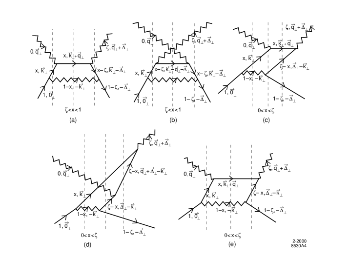
Figure 6: Light-cone time-ordered contributions to deeply virtual Compton scattering on an electron in QED at one-loop order. Note that the contribution of figure (e) is suppressed at large $q^{2}$ since the hard propagator with transverse momentum ${\vec{k}}_{\perp}+{\vec{q}}_{\perp}$ extends over two light-cone time orderings. The contributions of figures (c) and (d) correspond to the overlap of one-particle and three-particle Fock states. The three-particle Fock states occurs at the intermediate light-cone time indicated by the middle vertical dashed line.

The physical electron is the eigenstate of the QED Hamiltonian. As discussed in Section 4, the expansion of the QED eigenfunction of the electron on the complete set $\{|\,{n}\rangle\}$ of $H_{LC}(e=0)$ eigenstates produces the Fock state expansion. Each Fock-state wavefunction of the physical electron with total spin projection $J^{z}=\pm{1\over 2}$ is represented by the function $\psi^{J^{z}}_{n}(x_{i},{\vec{k}}_{\perp i},\lambda_{i})$, where

$$k_{i}=(k^{+}_{i},{\vec{k}}_{\perp i},k^{-}_{i})=\left(x_{i}P^{+},{\vec{k}}^{~{}}_{\perp i},\frac{{\vec{k}}_{\perp i}^{2}+m_{i}^{2}}{x_{i}P^{+}}\right)$$ (45)

specifies the momentum of each constituent and $\lambda_{i}$ specifies its light-cone helicity in the $z$ direction.

The quantum fluctuations of the electron at one-loop generate two types of light-cone wavefunctions, $|\,{e^{-}\gamma}\rangle$ and $|\,{e^{-}e^{-}e^{+}}\rangle$, in addition to renormalizing the one-electron state. The two-particle Fock state for an electron with $J^{z}=+{1\over 2}$ has four possible spin combinations for the electron and photon in flight:

$$\left|\Psi^{\uparrow}_{\rm two\ particle}(P^{+},\vec{P}_{\perp}=\vec{0}_{\perp})\right>=\int\frac{{\mathrm{d}}x\,{\mathrm{d}}^{2}{\vec{k}}_{\perp}}{\sqrt{x(1-x)}\,16\pi^{3}}$$

$$\left[\ \ \,\psi^{\uparrow}_{+\frac{1}{2}\,+1}(x,{\vec{k}}_{\perp})\,\left|+\frac{1}{2}\,+1\,;\,\,xP^{+}\,,\,\,{\vec{k}}_{\perp}\right>+\psi^{\uparrow}_{+\frac{1}{2}\,-1}(x,{\vec{k}}_{\perp})\,\left|+\frac{1}{2}\,-1\,;\,\,xP^{+}\,,\,\,{\vec{k}}_{\perp}\right>\right.$$

$$\left.{}+\psi^{\uparrow}_{-\frac{1}{2}\,+1}(x,{\vec{k}}_{\perp})\,\left|-\frac{1}{2}\,+1\,;\,\,xP^{+}\,,\,\,{\vec{k}}_{\perp}\right>+\psi^{\uparrow}_{-\frac{1}{2}\,-1}(x,{\vec{k}}_{\perp})\,\left|-\frac{1}{2}\,-1\,;\,\,xP^{+}\,,\,\,{\vec{k}}_{\perp}\right>\ \right]\ ,$$

where the two-particle states $|s_{\rm f}^{z},s_{\rm b}^{z};\ x,{\vec{k}}_{\perp}\rangle$ are normalized as in (36). $s_{\rm f}^{z}$ and $s_{\rm b}^{z}$ denote the $z$-component of the spins of the constituent fermion and boson, respectively, and the variables $x$ and ${\vec{k}}_{\perp}$ refer to the momentum of the fermion. The wavefunctions can be evaluated explicitly in QED perturbation theory using the rules given in Refs. [14, 16]:

$$\left\{\begin{array}[]{l}\psi^{\uparrow}_{+\frac{1}{2}\,+1}(x,{\vec{k}}_{\perp})=-{\sqrt{2}}\ \frac{-k^{1}+{i}k^{2}}{x(1-x)}\,\varphi\ ,\\ \psi^{\uparrow}_{+\frac{1}{2}\,-1}(x,{\vec{k}}_{\perp})=-{\sqrt{2}}\ \frac{k^{1}+{i}k^{2}}{1-x}\,\varphi\ ,\\ \psi^{\uparrow}_{-\frac{1}{2}\,+1}(x,{\vec{k}}_{\perp})=-{\sqrt{2}}\ (M-{m\over x})\,\varphi\ ,\\ \psi^{\uparrow}_{-\frac{1}{2}\,-1}(x,{\vec{k}}_{\perp})=0\ ,\end{array}\right.$$ (47)

where

$$\varphi(x,{\vec{k}}_{\perp})=\frac{e}{\sqrt{1-x}}\ \frac{1}{M^{2}-{{\vec{k}}_{\perp}^{2}+m^{2}\over x}-{{\vec{k}}_{\perp}^{2}+\lambda^{2}\over 1-x}}\ .$$ (48)

Similarly, the wavefunctions for an electron with negative helicity are given by

$$\left\{\begin{array}[]{l}\psi^{\downarrow}_{+\frac{1}{2}\,+1}(x,{\vec{k}}_{\perp})=0\ ,\\ \psi^{\downarrow}_{+\frac{1}{2}\,-1}(x,{\vec{k}}_{\perp})=-{\sqrt{2}}\ (M-{m\over x})\,\varphi\ ,\\ \psi^{\downarrow}_{-\frac{1}{2}\,+1}(x,{\vec{k}}_{\perp})=-{\sqrt{2}}\ \frac{-k^{1}+{i}k^{2}}{1-x}\,\varphi\ ,\\ \psi^{\downarrow}_{-\frac{1}{2}\,-1}(x,{\vec{k}}_{\perp})=-{\sqrt{2}}\ \frac{k^{1}+{i}k^{2}}{x(1-x)}\,\varphi\ .\end{array}\right.$$ (49)

In (47) and (49) we have generalized the framework of QED by assigning a mass $M$ to the external electrons in the Compton scattering process, but a different mass $m$ to the internal electron lines and a mass $\lambda$ to the internal photon line [16]. The idea behind this is to model the structure of a composite fermion state with mass $M$ by a fermion and a vector constituent with respective masses $m$ and $\lambda$.

In the domain $\zeta<x<1$, for a general value of $\zeta$ between 0 and 1, we have

$${\sqrt{1-\zeta}\over 1-{\zeta\over 2}}\ H_{(2\to 2)}(x,\zeta,t)\,-\,{\zeta^{2}\over 4(1-{\zeta\over 2}){\sqrt{1-\zeta}}}\ E_{(2\to 2)}(x,\zeta,t)$$

$$= \int\frac{{\mathrm{d}}^{2}{\vec{k}}_{\perp}}{16\pi^{3}}\Big{[}\psi^{\uparrow\ *}_{+\frac{1}{2}\,+1}(x^{\prime},{\vec{k}^{\prime}}_{\perp})\psi^{\uparrow}_{+\frac{1}{2}\,+1}(x,{\vec{k}}_{\perp})+\psi^{\uparrow\ *}_{+\frac{1}{2}\,-1}(x^{\prime},{\vec{k}^{\prime}}_{\perp})\psi^{\uparrow}_{+\frac{1}{2}\,-1}(x,{\vec{k}}_{\perp})$$

$$\qquad\qquad\qquad\qquad{}+\psi^{\uparrow\ *}_{-\frac{1}{2}\,+1}(x^{\prime},{\vec{k}^{\prime}}_{\perp})\psi^{\uparrow}_{-\frac{1}{2}\,+1}(x,{\vec{k}}_{\perp})\Big{]}\ ,$$

$${1\over\sqrt{1-\zeta}}\;{(\Delta^{1}-{i}\Delta^{2})\over 2M}\ E_{(2\to 2)}(x,\zeta,t)$$

$$= \int\frac{{\mathrm{d}}^{2}{\vec{k}}_{\perp}}{16\pi^{3}}\Big{[}\psi^{\uparrow\ *}_{+\frac{1}{2}\,-1}(x^{\prime},{\vec{k}^{\prime}}_{\perp})\psi^{\downarrow}_{+\frac{1}{2}\,-1}(x,{\vec{k}}_{\perp})+\psi^{\uparrow\ *}_{-\frac{1}{2}\,+1}(x^{\prime},{\vec{k}^{\prime}}_{\perp})\psi^{\downarrow}_{-\frac{1}{2}\,+1}(x,{\vec{k}}_{\perp})\Big{]}\ ,$$

where

$$x^{\prime}={x-\zeta\over 1-\zeta},\ \ \ {\vec{k}^{\prime}}_{\perp}={\vec{k}}^{~{}}_{\perp}-{1-x\over 1-\zeta}\ {\vec{\Delta}}_{\perp}\ .$$ (52)

These contributions correspond to the overlap of the two-particle Fock components of the electron as illustrated in Figs. 6(a) and 6(b). The generalized form factors $H_{(2\to 2)}(x,\zeta,t)$ and $E_{(2\to 2)}(x,\zeta,t)$ are zero in the domain $\zeta-1<x<0$, which corresponds to emission and reabsorption of an $e^{+}$ from a physical electron. Contributions to $H_{(n\to n)}(x,\zeta,t)$ and $E_{(n\to n)}(x,\zeta,t)$ in that domain only appear beyond one-loop level.

At this point, a comment is in order on the large ${\vec{k}}_{\perp}$ behavior of the overlap integrals (5) and (5). They are logarithmically divergent, which reflects the fact that the matrix elements defining parton distributions have to be regulated and renormalized in the ultraviolet. The dependence of parton distributions on the renormalization scale can be calculated perturbatively and is expressed in the well-known evolution equations. A physically intuitive way to implement this in our context is to introduce an upper cutoff in the invariant mass of the Fock states [14], which roughly speaking corresponds to an upper cutoff in the transverse parton momenta. How this is to be done in detail, and how it leads to the evolution equations for the generalized Compton form factors [1, 2, 3] is beyond the scope of the present paper.

We will also require three-constituent wavefunctions corresponding to two electrons and one positron in flight:

$$\psi^{J^{z}}_{{}_{s^{z}_{1}\,\,s^{z}_{2}\,\,s^{z}_{3}}}(x_{1},x_{2},x_{3},{\vec{k}}_{1\perp},{\vec{k}}_{2\perp},{\vec{k}}_{3\perp})=M^{J^{z}}_{s^{z}_{1}\,\,s^{z}_{2}\,\,s^{z}_{3}}\ {\widetilde{\varphi}}(x_{1},x_{2},x_{3},{\vec{k}}_{1\perp},{\vec{k}}_{2\perp},{\vec{k}}_{3\perp}),$$ (53)

where according to our numbering convention spelled out after (44) the index $1$ refers to the electron with mass $m$, the index $2$ to the electron with mass $M$, and the index $3$ to the positron. The denominator part of the wavefunction ${\widetilde{\varphi}}$ is given by

$${\widetilde{\varphi}}(x_{1},x_{2},x_{3},{\vec{k}}_{1\perp},{\vec{k}}_{2\perp},{\vec{k}}_{3\perp})={e^{2}\over 1-x_{1}}$$

$${}\times{1\over\left(M^{2}-{m^{2}+{\vec{k}}_{1\perp}^{2}\over x_{1}}-{\lambda^{2}+{\vec{k}}_{1\perp}^{2}\over 1-x_{1}}\right)\left(M^{2}-{m^{2}+{\vec{k}}_{1\perp}^{2}\over x_{1}}-{M^{2}+{\vec{k}}_{2\perp}^{2}\over x_{2}}-{m^{2}+{\vec{k}}_{3\perp}^{2}\over x_{3}}\right)}\ .$$

The numerator factors $M^{J^{z}}_{s^{z}_{1}\,\,s^{z}_{2}\,\,s^{z}_{3}}$ in (53) in QED are given in Table 1.

In the wave functions (53) the positron and the electron with index $2$ originate in the splitting of the intermediate photon, corresponding to the diagrams of Fig 6(c) and (d). We note that there is also a contribution to the three-particle wavefunctions where the photon splits into the positron and the electron with index $1$. These terms do not contribute to deeply virtual Compton scattering because of charge conjugation invariance; see Fig. 7(a). They do contribute in the calculation of the electromagnetic vertex as shown in Fig. 7(b), where they provide the vacuum polarization correction for the external photon. This correction is usually excluded in the definition of the electromagnetic form factors $F_{1}$ and $F_{2}$, and thus of the first moments of $H$ and $E$. We will therefore discard the corresponding contributions to $H(x,\zeta,t)$ and $E(x,\zeta,t)$ in the following.

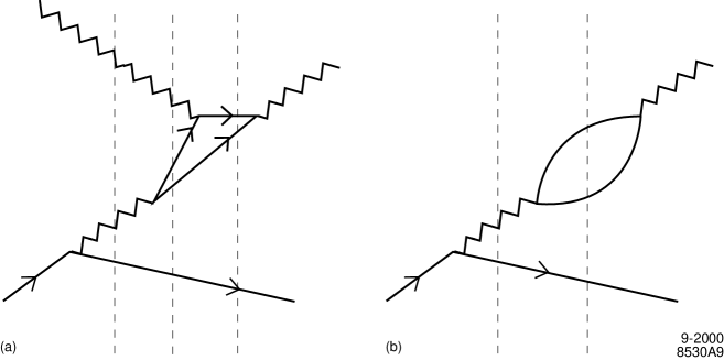
Figure 7: Light-cone time-ordered diagrams where the electron coupling to the external current originates from the splitting of an intermediate photon. Diagram (a) for deeply virtual Compton scattering vanishes because of Furry’s theorem. The corresponding diagram (b) for the electromagnetic vertex gives the vacuum polarization correction for the external photon.

Table 1. Numerator factors of the three-constituent wavefunctions in QED. We only list those helicity combinations for which $s_{1}^{z}=-s_{3}^{z}$.

$\ \ \ \ J^{z}\ \ \ \$	$\ \ s^{z}_{1}\ \ \ \ s^{z}_{2}\ \ \ \ s^{z}_{3}\ \$	$\ \ \ {1\over 2}\ M^{J^{z}}_{s^{z}_{1}\,\,s^{z}_{2}\,\,s^{z}_{3}}\ \ \$
$+{1\over 2}$	$\ \ +{1\over 2}\ \ +{1\over 2}\ \ -{1\over 2}\ \$	$-\frac{k_{1}^{1}-{i}k_{1}^{2}}{x_{1}(1-x_{1})}\,({k_{3}^{1}+{i}k_{3}^{2}\over x_{3}}+{k_{1}^{1}+{i}k_{1}^{2}\over 1-x_{1}})\,-\,\frac{k_{1}^{1}+{i}k_{1}^{2}}{1-x_{1}}\,({k_{2}^{1}-{i}k_{2}^{2}\over x_{2}}+{k_{1}^{1}-{i}k_{1}^{2}\over 1-x_{1}})$
$+{1\over 2}$	$\ \ -{1\over 2}\ \ +{1\over 2}\ \ +{1\over 2}\ \$	$-(M-{m\over x_{1}})\,({M\over x_{2}}+{m\over x_{3}})$
$+{1\over 2}$	$\ \ +{1\over 2}\ \ -{1\over 2}\ \ -{1\over 2}\ \$	$-\frac{k_{1}^{1}+{i}k_{1}^{2}}{1-x_{1}}\,({M\over x_{2}}+{m\over x_{3}})$
$+{1\over 2}$	$\ \ -{1\over 2}\ \ -{1\over 2}\ \ +{1\over 2}\ \$	$(M-{m\over x_{1}})\,({k_{2}^{1}+{i}k_{2}^{2}\over x_{2}}+{k_{1}^{1}+{i}k_{1}^{2}\over 1-x_{1}})$
$-{1\over 2}$	$\ \ +{1\over 2}\ \ +{1\over 2}\ \ -{1\over 2}\ \$	$-(M-{m\over x_{1}})\,({k_{2}^{1}-{i}k_{2}^{2}\over x_{2}}+{k_{1}^{1}-{i}k_{1}^{2}\over 1-x_{1}})$
$-{1\over 2}$	$\ \ -{1\over 2}\ \ +{1\over 2}\ \ +{1\over 2}\ \$	$\frac{k_{1}^{1}-{i}k_{1}^{2}}{1-x_{1}}\,({M\over x_{2}}+{m\over x_{3}})$
$-{1\over 2}$	$\ \ +{1\over 2}\ \ -{1\over 2}\ \ -{1\over 2}\ \$	$-(M-{m\over x_{1}})\,({M\over x_{2}}+{m\over x_{3}})$
$-{1\over 2}$	$\ \ -{1\over 2}\ \ -{1\over 2}\ \ +{1\over 2}\ \$	$-\frac{k_{1}^{1}+{i}k_{1}^{2}}{x_{1}(1-x_{1})}\,({k_{3}^{1}-{i}k_{3}^{2}\over x_{3}}+{k_{1}^{1}-{i}k_{1}^{2}\over 1-x_{1}})\,-\,\frac{k_{1}^{1}-{i}k_{1}^{2}}{1-x_{1}}\,({k_{2}^{1}+{i}k_{2}^{2}\over x_{2}}+{k_{1}^{1}+{i}k_{1}^{2}\over 1-x_{1}})$

The electron in QED also has a one-particle component:

$$\left|\Psi_{\rm one\ particle}^{\uparrow,\downarrow}(P^{+},\vec{P}_{\perp}=\vec{0}_{\perp})\right>=\int{{\mathrm{d}}x\,{\mathrm{d}}^{2}{\vec{k}}_{\perp}\over\sqrt{x}\,16\pi^{3}}\ 16\pi^{3}\delta(1-x)\,{\delta}^{2}({\vec{k}}_{\perp})\ \psi_{(1)}\ \left|\pm{1\over 2}\,;xP^{+},{\vec{k}}_{\perp}\right>$$ (55)

where the one-constituent wavefunction is given by

$$\psi_{(1)}=\sqrt{Z}.$$ (56)

Here $\sqrt{Z}$ is the wavefunction renormalization of the one-particle state and ensures overall probability conservation. Since we are working consistently to ${\cal O}(\alpha)$, we can set $Z=1$ in the $3\to 1$ wavefunction overlap contributions. In the domain $0<x<\zeta$, we then have

$${\sqrt{1-\zeta}\over 1-{\zeta\over 2}}\ H_{(3\to 1)}(x,\zeta,t)\,-\,{\zeta^{2}\over 4(1-{\zeta\over 2}){\sqrt{1-\zeta}}}\ E_{(3\to 1)}(x,\zeta,t)$$

$$= \sqrt{1-\zeta}\,\int{{\rm d}^{2}{\vec{k}}_{\perp}\over 16\pi^{3}}\ \left[\psi^{\uparrow}_{{}_{+{1\over 2}\,\,+{1\over 2}\,\,-{1\over 2}}}(x,1-\zeta,\zeta-x,\ {\vec{k}}_{\perp},-{\vec{\Delta}}_{\perp},{\vec{\Delta}}_{\perp}-{\vec{k}}_{\perp})\right.$$

$$\hskip 64.00003pt\left.{}+\psi^{\uparrow}_{{}_{-{1\over 2}\,\,+{1\over 2}\,\,+{1\over 2}}}(x,1-\zeta,\zeta-x,{\vec{k}}_{\perp},-{\vec{\Delta}}_{\perp},{\vec{\Delta}}_{\perp}-{\vec{k}}_{\perp})\right]\ ,$$

$${1\over\sqrt{1-\zeta}}\;{(\Delta^{1}-{i}\Delta^{2})\over 2M}\ E_{(3\to 1)}(x,\zeta,t)$$

$$= \sqrt{1-\zeta}\,\int{{\rm d}^{2}{\vec{k}}_{\perp}\over 16\pi^{3}}\ \left[\psi^{\downarrow}_{{}_{+{1\over 2}\,\,+{1\over 2}\,\,-{1\over 2}}}(x,1-\zeta,\zeta-x,\ {\vec{k}}_{\perp},-{\vec{\Delta}}_{\perp},{\vec{\Delta}}_{\perp}-{\vec{k}}_{\perp})\right.$$

$$\hskip 64.00003pt\left.{}+\psi^{\downarrow}_{{}_{-{1\over 2}\,\,+{1\over 2}\,\,+{1\over 2}}}(x,1-\zeta,\zeta-x,{\vec{k}}_{\perp},-{\vec{\Delta}}_{\perp},{\vec{\Delta}}_{\perp}-{\vec{k}}_{\perp})\right]\ .$$

These contributions correspond to the overlap of the three-particle and one-particle Fock components as illustrated in Figs. 6(c) and 6(d).

The first moments (3) and (3) of the generalized Compton form factors at one loop give the one-loop space-like form factors $F_{1}$ and $F_{2}$. The corresponding light-cone time-ordered diagrams are shown in Fig. 8. As in our simple example discussed at the end of Section 4, the sum of the two diagrams must give the same result as the corresponding Feynman diagram in covariant perturbation theory. The division of the integral over $x$ in the form factors (3) and (3) into contributions from $n\to n$ and $n+1\to n-1$ transitions is again a consequence of an arbitrary choice of frame and of light-cone direction, and the sum of the contributions is thus independent of the light-cone variable $\zeta$.

We also note that the integrands in (3) and (3) have to be continuous at the point $x=\zeta$ which separates $n\to n$ and $n+1\to n-1$ transitions. In other words, the generalized form factors $H(x,\zeta,t)$ and $E(x,\zeta,t)$ must be continuous functions of $x$ at $x=\zeta$. This is required for the loop integral (3) of the Compton amplitude to exist, given the form (13) of the hard scattering subprocess. The continuity of $H$ and $E$ in one-loop QED can readily be checked from our results (5), (5), (5), (5). The underlying relations between the one, two, and three particle wavefunctions of the electron reflect again the Lorentz frame invariance of the light-cone Fock state representation.

Figure 8: Light-cone time-ordered contributions to the form factors of an electron in QED at one-loop order. The spacelike form factors are independent of the choice of $\zeta$ at fixed $t=\Delta^{2}$. In particular, if $\zeta=0$ the contribution of amplitude (c) to the matrix elements of $J^{+}(0)$ vanishes.

6 Conclusions

A central goal of quantum chromodynamics is to determine the structure of hadrons in terms of their quark and gluon degrees of freedom. As we have shown in this paper, the deeply virtual Compton exclusive process $\gamma^{*}p\to\gamma p$ provides a direct window into hadron substructure which goes well beyond inclusive measures.

The deeply virtual Compton amplitude has a simple representation in terms of the light-cone Fock wavefunctions of the target, factorizing as the convolution of a hard perturbative amplitude, corresponding to Compton scattering on a quark current, with the initial and final state light-cone wavefunctions of the target hadron. The light-cone Fock representation provides an explicit and physical representation of the leading-twist operator product decomposition for the deeply virtual Compton amplitude. As in the case of time-like semi-leptonic decays of hadrons [18], there are two distinct contributions: a parton-number conserving diagonal overlap integral of light-cone wavefunctions, plus an additional $\Delta n=-2$ contribution where the quark-antiquark pair of the initial state is annihilated.

The light-cone Fock representation also provides a direct derivation of the identity between the form factor densities $H(x,\zeta,t)$ and $E(x,\zeta,t)$ which appear in deeply virtual Compton scattering and the corresponding integrands of the Dirac and Pauli form factors $F_{1}(t)$ and $F_{2}(t)$, and the gravitational form factors $A_{q}(t)$ and $B_{q}(t)$ for each quark and anti-quark constituent. Thus deeply virtual Compton scattering effectively provides access to the form factors of a proton scattering in a gravitational field.

A remarkable feature of these sum rules is the fact that the integrals over $x$ of $(1-\zeta/2)^{-1}\,H(x,\zeta,t)$ and $(1-\zeta/2)^{-1}\,E(x,\zeta,t)$ are independent of the value of $\zeta$. This invariance is due to the Lorentz frame-independence of the light-cone Fock representation of space-like local operator matrix elements. This frame independence in turn reflects the underlying connections between Fock states of different parton number implied by the QCD equations of motion.

We have illustrated our general formalism by computing deeply virtual Compton scattering on the quantum fluctuations of a fermion in QED at one loop. These forms can be simply generalized using Pauli-Villars spectral integrals to provide a self-consistent model of hadron structure. Such a model builds in all of the constraints of Lorentz invariance, including $J^{z}$ conservation and the required connections of the $n$, $n-1$, and $n+1$-particle Fock states. Such a model thus provides the simplest possible template for parametrizing and interrelating hadronic structure as measured by form factors, deep inelastic scattering and deeply virtual Compton scattering.

Appendix: Formulae in the Symmetric Frame

It is often convenient to choose a “symmetric” light-cone frame for the momenta of the initial and final target proton which has $\Delta\to-\Delta$ symmetry. In this frame, one parametrizes the initial and final target momenta as [2]:

$$P=\left((1+\xi){\bar{P}}^{+}\ ,\ {\vec{\Delta}_{\perp}/2}\ ,\ {M^{2}+{\vec{\Delta}_{\perp}}^{2}/4\over(1+\xi){\bar{P}}^{+}}\right)\ ,$$ (59)

$$P^{\prime}=\left((1-\xi){\bar{P}}^{+}\ ,\ -{\vec{\Delta}_{\perp}/2}\ ,\ {M^{2}+{\vec{\Delta}_{\perp}}^{2}/4\over(1-\xi){\bar{P}}^{+}}\right)\ .$$ (60)

The four-momentum transfer from the target then reads

$$\Delta\ =\left(2\xi{\bar{P}}^{+}\ ,\ {\vec{\Delta}_{\perp}}\ ,\ {(t+{\vec{\Delta}_{\perp}}^{2})\over 2\xi{\bar{P}}^{+}}\right)\ ,$$ (61)

and one has

$$t=-{4\xi^{2}M^{2}+{\vec{\Delta}_{\perp}}^{2}\over 1\ -\ \xi^{2}}\ .$$ (62)

Notice that our definition of the transfer $\Delta$ has the opposite sign of Ji’s. Again we choose a light-cone frame where the incident space-like photon carries $q^{+}=0$:

$$q = \left(0\ ,\ {\vec{q}_{\perp}}\ ,\ {({\vec{q}_{\perp}}+{\vec{\Delta}_{\perp}})^{2}\over 2\xi{\bar{P}}^{+}}+{2\xi(M^{2}+{\vec{\Delta}_{\perp}}^{2}/4)\over(1-\xi^{2}){\bar{P}}^{+}}\right)\ ,$$ (63)

$$q^{\prime} = \left(2\xi{\bar{P}}^{+}\ ,\ {\vec{q}_{\perp}}+{\vec{\Delta}_{\perp}}\ ,\ {({\vec{q}_{\perp}}+{\vec{\Delta}_{\perp}})^{2}\over 2\xi{\bar{P}}^{+}}\right)\ .$$

In the same way as in Section 2 one can relate $\xi$ to the invariants of the problem. Taking the limit of large $Q^{2}$ at small $t$ and comparing with (9) we obtain the relation

$$\zeta={2\xi\over 1+\xi}\ .$$ (64)

We remark that the symmetric frame just introduced and the one described by (2) to (7) are related by a transverse boost. One finds that the transverse components of $\Delta$ in the two frames are related by

$$\vec{\Delta}_{\perp}\Big{|}_{\mathrm{E}q.~{}(\ref{delta})}={1\over 1+\xi}\ \vec{\Delta}_{\perp}\Big{|}_{\mathrm{E}q.~{}(\ref{app3})}\ .$$ (65)

The deeply virtual Compton amplitude can now be written as

$$M^{IJ}({\vec{q}_{\perp}},{\vec{\Delta}_{\perp}},\zeta)\ =\ -e^{2}_{q}\ {1\over 2\bar{P}^{+}}\int_{-1}^{1}d{\bar{x}}\$$

$$\times \left\{\ {\bar{t}}^{IJ}({\bar{x}},\xi)\ {\bar{U}}(P^{\prime})\left[H({\bar{x}},\xi,t)\ {\gamma^{+}}+E({\bar{x}},\xi,t)\ {i\over 2M}\,{\sigma^{+\alpha}}(-\Delta_{\alpha})\right]U(P)\right.$$

$$\ \ \left.{\bar{s}}^{IJ}({\bar{x}},\xi)\ {\bar{U}}(P^{\prime})\left[{\widetilde{H}}({\bar{x}},\xi,t)\ {\gamma^{+}\gamma_{5}}+{\widetilde{E}}({\bar{x}},\xi,t)\ {1\over 2M}\,{\gamma_{5}}(-\Delta^{+})\right]U(P)\ \right\}$$

with

$${\bar{t}}^{\ \uparrow\uparrow}({\bar{x}},\xi) = \phantom{-}\ {\bar{t}}^{\ \downarrow\downarrow}({\bar{x}},\xi)\ =\ {1\over{\bar{x}}+\xi-i\epsilon}\ +\ {1\over{\bar{x}}-\xi+i\epsilon}\ ,$$ (67)

$${\bar{s}}^{\ \uparrow\uparrow}({\bar{x}},\xi) = -\ {\bar{s}}^{\ \downarrow\downarrow}({\bar{x}},\xi)\ =\ {1\over{\bar{x}}+\xi-i\epsilon}\ -\ {1\over{\bar{x}}-\xi+i\epsilon}\ ,$$

$${\bar{t}}^{\ \uparrow\downarrow}({\bar{x}},\xi) = {\bar{t}}^{\ \downarrow\uparrow}({\bar{x}},\xi)\ =\ {\bar{s}}^{\ \uparrow\downarrow}({\bar{x}},\xi)\ =\ {\bar{s}}^{\ \downarrow\uparrow}({\bar{x}},\xi)\ \ =\ \ 0\ \phantom{\frac{1}{2}}.$$

for circularly polarized photons. The variable $\bar{x}$ is related to $x$ in Section 3 by

$$x=\frac{\bar{x}+\xi}{1+\xi}$$ (68)

and is again chosen such as to make symmetry relations under $\Delta\to-\Delta$ most transparent.

Using the transformation rules (64), (65), and (68) it is straightforward to translate all our results into the variables in the symmetric frame. For convenience, we give in the following our main formulae explicitly. The spinor products in (21) and (24) now read

$${1\over 2\bar{P}^{+}}\ {\bar{U}}(P^{\prime},{\lambda}^{\prime}){\gamma^{+}}\,U(P,\lambda) = {\sqrt{1-\xi^{2}}}\ \delta_{\lambda,\,{\lambda}^{\prime}}\ ,$$ (69)

$${1\over 2\bar{P}^{+}}\ {\bar{U}}(P^{\prime},{\lambda}^{\prime}){i\over 2M}\,{\sigma^{+\alpha}}(-\Delta_{\alpha})U(P,\lambda) = -\,{\xi^{2}\over\sqrt{1-\xi^{2}}}\ \delta_{\lambda,\,{\lambda}^{\prime}}$$

$$+\ {1\over\sqrt{1-\xi^{2}}}\;{\,-\lambda\Delta^{1}\,-\,i\Delta^{2}\,\over 2M}\ \delta_{\lambda,\,-{\lambda}^{\prime}}\ ,$$

$${1\over 2M}\ {\bar{U}}(P^{\prime},{\lambda}^{\prime})U(P,\lambda) = {1\over{\sqrt{1-\xi^{2}}}}\ \delta_{\lambda,\,{\lambda}^{\prime}}$$ (70)

$$-{1\over{\sqrt{1-\xi^{2}}}}\;{-\lambda\Delta^{1}\,-\,i\Delta^{2}\over 2M}\ \delta_{\lambda,\,-{\lambda}^{\prime}}\ ,$$

and the sum rules for the form factors take the simple forms

$$\int_{-1}^{1}d{\bar{x}}\ H(\bar{x},\xi,t) = F_{1}(t)\ ,$$ (71)

$$\int_{-1}^{1}d{\bar{x}}\ E(\bar{x},\xi,t) = F_{2}(t)\ ,$$

$$\int_{-1}^{1}d{\bar{x}}\,{\bar{x}}\,[\,H(\bar{x},\xi,t)+E(\bar{x},\xi,t)\,] = A_{q}(t)+B_{q}(t)\ .$$

The Fock state representations of the Compton form factors $H$ and $E$ are again more symmetric with respect to the initial and final state proton if we use the variables of the symmetric frame, although at the price of somewhat more involved relations between the different momentum variables. For the $n\to n$ diagonal term ($\Delta n=0$) we obtain in the domain $\xi\leq{\bar{x}}\leq 1$:

$${\sqrt{1-\xi^{2}}}\ H_{(n\to n)}(\bar{x},\xi,t)\,-\,{\xi^{2}\over{\sqrt{1-\xi^{2}}}}\,E_{(n\to n)}(\bar{x},\xi,t)$$

$$= \sqrt{1-\xi}^{\,2-n}\sqrt{1+\xi}^{\,2-n}\,\sum_{n,\lambda_{i}}\int\prod_{i=1}^{n}{{\rm d}x_{i}\,{\rm d}^{2}{\vec{k}}_{\perp i}\over 16\pi^{3}}\ 16\pi^{3}\delta\left(1-\sum_{j=1}^{n}x_{j}\right)\,\delta^{(2)}\left(\sum_{j=1}^{n}{\vec{k}}_{\perp j}\right)$$

$$\times\delta({\bar{x}}-x_{1})\ \psi^{\uparrow\ *}_{(n)}(x^{\prime}_{i},{\vec{k}}^{\prime}_{\perp i},\lambda_{i})~{}\psi^{\uparrow}_{(n)}(y_{i},{\vec{l}}_{\perp i},\lambda_{i}),$$

$${1\over{\sqrt{1-\xi^{2}}}}\,{\Delta^{1}-{i}\Delta^{2}\over 2M}\ E_{(n\to n)}(\bar{x},\xi,t)$$

$$= \sqrt{1-\xi}^{\,2-n}\sqrt{1+\xi}^{\,2-n}\,\sum_{n,\lambda_{i}}\int\prod_{i=1}^{n}{{\rm d}x_{i}\,{\rm d}^{2}{\vec{k}}_{\perp i}\over 16\pi^{3}}\ 16\pi^{3}\delta\left(1-\sum_{j=1}^{n}x_{j}\right)\,\delta^{(2)}\left(\sum_{j=1}^{n}{\vec{k}}_{\perp j}\right)$$

$$\times\delta({\bar{x}}-x_{1})\ \psi^{\uparrow\ *}_{(n)}(x^{\prime}_{i},{\vec{k}}^{\prime}_{\perp i},\lambda_{i})~{}\psi^{\downarrow}_{(n)}(y_{i},{\vec{l}}_{\perp i},\lambda_{i}),$$

where

$$\begin{array}[t]{lll}x^{\prime}_{1}=\displaystyle\frac{{x_{1}}-\xi}{1-\xi}\,,&{\vec{k}}^{\prime}_{\perp 1}={\vec{k}}_{\perp 1}-\displaystyle\frac{1-x_{1}}{1-\xi}\,\frac{\vec{\Delta}_{\perp}}{2}&\mbox{for the final struck quark,}\\[4.30554pt] x^{\prime}_{i}=\displaystyle\frac{x_{i}}{1-\xi}\,,&{\vec{k}}^{\prime}_{\perp i}={\vec{k}}_{\perp i}+\displaystyle\frac{x_{i}}{1-\xi}\,\frac{\vec{\Delta}_{\perp}}{2}&\mbox{for the final $(n-1)$ spectators,}\end{array}$$ (74)

and

$$\begin{array}[t]{lll}y_{1}=\displaystyle\frac{x_{1}+\xi}{1+\xi}\,,&{\vec{l}}_{\perp 1}={\vec{k}}_{\perp 1}+\displaystyle\frac{1-x_{1}}{1+\xi}\,\frac{\vec{\Delta}_{\perp}}{2}&\mbox{for the initial struck quark,}\\[4.30554pt] y_{i}=\displaystyle\frac{x_{i}}{1+\xi}\,,&{\vec{l}}_{\perp i}={\vec{k}}_{\perp i}-\displaystyle\frac{x_{i}}{1+\xi}\,\frac{\vec{\Delta}_{\perp}}{2}&\mbox{for the initial $(n-1)$ spectators.}\end{array}$$ (75)

We can again check that $\sum_{i=1}^{n}x^{\prime}_{i}=1$ and $\sum_{i=1}^{n}{\vec{k}}^{\prime}_{\perp i}={\vec{0}}_{\perp}$. We also have $\sum^{n}_{i=1}y_{i}=1$ and $\sum^{n}_{i=1}{\vec{l}}_{\perp i}={\vec{0}}_{\perp}$ as required. From (74) and (75) we see that the variable $\bar{x}=x_{1}$ corresponds to the average momentum fraction $(y_{1}P^{+}+x^{\prime}_{1}P^{\prime+})/(P^{+}+P^{\prime+})$ of the struck quark before and after the scattering.

For the $n+1\to n-1$ off-diagonal term ($\Delta n=-2$), let us consider the case where partons $1$ and $n+1$ of the initial wavefunction annihilate into the current leaving $n-1$ spectators. The final state $n-1$ parton wavefunction then has arguments $(i=2,\cdots,n)$

$$x^{\prime}_{i}={x_{i}\over 1-\xi}\ ,\qquad{\vec{k}}^{\prime}_{\perp i}={\vec{k}}_{\perp i}+{x_{i}\over 1-\xi}\frac{\vec{\Delta}_{\perp}}{2}\ .$$ (76)

We can check that $\sum_{i=2}^{n}x^{\prime}_{i}=1$ and $\sum_{i=2}^{n}{\vec{k}}^{\prime}_{\perp i}={\vec{0}}_{\perp}$. The initial state $n+1$ parton wavefunction has arguments $(i=1,\cdots,n+1)$,

$$y_{1} = {x_{1}+\xi\over 1+\xi}\ ,\qquad\qquad\!{\vec{l}}_{\perp 1}\ =\ {\vec{k}}_{\perp 1}+{1-x_{1}\over 1+\xi}\,\frac{{\vec{\Delta}}_{\perp}}{2}\ ,$$ (77)

$$y_{n+1} = {x_{n+1}-\xi\over 1+\xi}\ ,\qquad\!{\vec{l}}_{\perp n+1}\ =\ {\vec{k}}_{\perp n+1}-{1+x_{n+1}\over 1+\xi}\,\frac{{\vec{\Delta}}_{\perp}}{2}\ ,$$

$$y_{i} = {x_{i}\over 1+\xi}\ ,\qquad\qquad\ {\vec{l}}_{\perp i}\ =\ {\vec{k}}_{\perp i}-{x_{i}\over 1+\xi}\,\frac{{\vec{\Delta}}_{\perp}}{2}\qquad\qquad{\rm for}\ i=2,\cdots,n\ .$$

This satisfies $\sum^{n+1}_{i=1}y_{i}=1$, $\sum^{n+1}_{i=1}{\vec{l}}_{\perp i}={\vec{0}}_{\perp}$ as required. The off-diagonal amplitude is non-zero in the domain $-\xi\leq\bar{x}\leq\xi$. There, the formulae for the generalized form factors of the deeply virtual Compton amplitude are

$${\sqrt{1-\xi^{2}}}\ H_{(n+1\to n-1)}(\bar{x},\xi,t)\,-\,{\xi^{2}\over{\sqrt{1-\xi^{2}}}}\ E_{(n+1\to n-1)}(\bar{x},\xi,t)$$

$$= \sqrt{1-\xi}^{\,3-n}\sqrt{1+\xi}^{\,1-n}\,\sum_{n,\lambda_{i}}\int\prod_{i=1}^{n+1}{{\rm d}x_{i}\,{\rm d}^{2}{\vec{k}}_{\perp i}\over 16\pi^{3}}\$$

$$\qquad\qquad\rule{0.0pt}{12.91663pt}{}\times 16\pi^{3}\delta\left(1+\xi-\sum_{j=1}^{n+1}x_{j}\right)\,\delta^{(2)}\left(\frac{{\vec{\Delta}}_{\perp}}{2}-\sum_{j=1}^{n+1}{\vec{k}}_{\perp j}\right)$$

$$\qquad\qquad\rule{0.0pt}{12.91663pt}{}\times 16\pi^{3}\delta(x_{n+1}+x_{1}-2\xi)\,\delta^{(2)}\left({\vec{k}}_{\perp n+1}+{\vec{k}}_{\perp 1}-{\vec{\Delta}}_{\perp}\right)$$

$$\qquad\qquad\rule{0.0pt}{12.91663pt}{}\times\delta({\bar{x}}-x_{1})\ \psi^{\uparrow\ *}_{(n-1)}(x^{\prime}_{i},{\vec{k}}^{\prime}_{\perp i},\lambda_{i})~{}\psi^{\uparrow}_{(n+1)}(y_{i},{\vec{l}}_{\perp i},\lambda_{i})\ \delta_{\lambda_{1}\,-\lambda_{n+1}}\ ,$$

$${1\over{\sqrt{1-\xi^{2}}}}\,{(\Delta^{1}-{i}\Delta^{2})\over 2M}\ E_{(n+1\to n-1)}(\bar{x},\xi,t)$$

$$= \sqrt{1-\xi}^{\,3-n}\sqrt{1+\xi}^{\,1-n}\,\sum_{n,\lambda_{i}}\int\prod_{i=1}^{n+1}{{\rm d}x_{i}\,{\rm d}^{2}{\vec{k}}_{\perp i}\over 16\pi^{3}}\$$

$$\qquad\qquad\rule{0.0pt}{12.91663pt}{}\times 16\pi^{3}\delta\left(1+\xi-\sum_{j=1}^{n+1}x_{j}\right)\,\delta^{(2)}\left(\frac{{\vec{\Delta}}_{\perp}}{2}-\sum_{j=1}^{n+1}{\vec{k}}_{\perp j}\right)$$

$$\qquad\qquad\rule{0.0pt}{12.91663pt}{}\times 16\pi^{3}\delta(x_{n+1}+x_{1}-2\xi)\,\delta^{(2)}\left({\vec{k}}_{\perp n+1}+{\vec{k}}_{\perp 1}-{\vec{\Delta}}_{\perp}\right)$$

$$\qquad\qquad\rule{0.0pt}{12.91663pt}{}\times\delta({\bar{x}}-x_{1})\ \psi^{\uparrow\ *}_{(n-1)}(x^{\prime}_{i},{\vec{k}}^{\prime}_{\perp i},\lambda_{i})~{}\psi^{\downarrow}_{(n+1)}(y_{i},{\vec{l}}_{\perp i},\lambda_{i})\ \delta_{\lambda_{1}\,-\lambda_{n+1}}\ .$$

References

[1]
D. Müller, D. Robaschik, B. Geyer, F. M. Dittes and
J. Hořejši,
Fortsch. Phys. 42, 101 (1994)
[hep-ph/9812448].
[2]
X. Ji,
Phys. Rev. Lett. 78, 610 (1997)
[hep-ph/9603249];
Phys. Rev. D55, 7114 (1997)
[hep-ph/9609381].
[3]
A. V. Radyushkin,
Phys. Rev. D56, 5524 (1997)
[hep-ph/9704207].
[4]
X. Ji,
J. Phys. G 24, 1181 (1998)
[hep-ph/9807358], and references therein.
[5]
J. Blümlein, B. Geyer and D. Robaschik,
Nucl. Phys. B560, 283 (1999)
[hep-ph/9903520];
J. Blümlein and D. Robaschik,
Nucl. Phys. B581, 449 (2000)
[hep-ph/0002071].
[6]
X. Ji and J. Osborne,
Phys. Rev. D58, 094018 (1998)
[hep-ph/9801260].
[7]
J. C. Collins and A. Freund,
Phys. Rev. D59, 074009 (1999)
[hep-ph/9801262].
[8]
S. J. Brodsky, F. E. Close and J. F. Gunion,
Phys. Rev. D5, 1384 (1972);
Phys. Rev. D6, 177 (1972);
Phys. Rev. D8, 3678 (1973).
[9]
P. Kroll, M. Schürmann and P. A. Guichon,
Nucl. Phys. A598, 435 (1996)
[hep-ph/9507298];
M. Diehl, T. Gousset, B. Pire and J. P. Ralston,
Phys. Lett. B411, 193 (1997)
[hep-ph/9706344];
A. V. Belitsky, D. Müller, L. Niedermeier and A. Schäfer,
hep-ph/0004059.
[10]
M. Diehl, T. Gousset and B. Pire,
Phys. Rev. D62, 073014 (2000)
[hep-ph/0003233], and references therein.
[11]
P. V. Landshoff, J. C. Polkinghorne and R. D. Short,
Nucl. Phys. B 28, 225 (1971).
[12]
M. Diehl and T. Gousset,
Phys. Lett. B428, 359 (1998)
[hep-ph/9801233].
[13]
S. J. Brodsky, D. S. Hwang, B. Ma and I. Schmidt,
hep-th/0003082.
[14]
G. P. Lepage and S. J. Brodsky,
Phys. Rev. D22, 2157 (1980);
S. J. Brodsky and G. P. Lepage,
in: Perturbative Quantum Chromodynamics, edited by
A. H. Mueller (World Scientific, Singapore 1989).
[15]
S. D. Drell and T. Yan,
Phys. Rev. Lett. 24, 181 (1970);
G. B. West,
Phys. Rev. Lett. 24, 1206 (1970).
[16]
S. J. Brodsky and S. D. Drell,
Phys. Rev. D 22, 2236 (1980).
[17]
M. Diehl, T. Feldmann, R. Jakob and P. Kroll,
Eur. Phys. J. C8, 409 (1999)
[hep-ph/9811253].
[18]
S. J. Brodsky and D. S. Hwang,
Nucl. Phys. B543, 239 (1999)
[hep-ph/9806358].
[19]
M. B. Einhorn,
Phys. Rev. D 14, 3451 (1976).
[20]
M. Burkardt,
Phys. Rev. D62, 094003 (2000)
[hep-ph/0005209].
[21]
L. Mankiewicz, G. Piller, E. Stein, M. Vänttinen and T. Weigl,
Phys. Lett. B425, 186 (1998)
[hep-ph/9712251];
A. V. Belitsky, D. Müller, L. Niedermeier and A. Schäfer,
Phys. Lett. B474, 163 (2000)
[hep-ph/9908337].
[22]
I. V. Anikin, B. Pire and O. V. Teryaev,
Phys. Rev. D62, 071501 (2000)
[hep-ph/0003203];
M. Penttinen, M. V. Polyakov, A. G. Shuvaev and M. Strikman,
Phys. Lett. B491, 96 (2000)
[hep-ph/0006321];
A. V. Belitsky and D. Müller,
Nucl. Phys. B589, 611 (2000)
[hep-ph/0007031];
N. Kivel, M. V. Polyakov, A. Schäfer and O. V. Teryaev,
hep-ph/0007315;
A. V. Radyushkin and C. Weiss,
hep-ph/0008214;
N. Kivel and M. V. Polyakov,
hep-ph/0010150;
A. V. Radyushkin and C. Weiss,
hep-ph/0010296.
[23]
I. Yu. Kobzarev and L. B. Okun,
Zh. Eksp. Teor. Fiz. 43, 1904 (1962),
Sov. Phys. JETP 16, 1343 (1963).
[24]
S. Gazek and M. Sawicki,
Phys. Rev. D41, 2563 (1990);
M. Sawicki,
Phys. Rev. D46, 474 (1992).
[25]
P. A. M. Dirac,
Rev. Mod. Phys. 21, 392 (1949);
S. J. Brodsky, H. Pauli and S. S. Pinsky,
Phys. Rept. 301, 299 (1998)
[hep-ph/9705477].
[26]
H. C. Pauli and S. J. Brodsky,
Phys. Rev. D32, 2001 (1985).
[27]
M. Diehl, T. Feldmann, R. Jakob and P. Kroll,
hep-ph/0009255.