September 2000 DPNU-00-29
Wilsonian Matching of Effective Field Theory
with Underlying QCD

Abstract

We propose a novel way of matching effective field theory with the underlying QCD in the sense of a Wilsonian renormalization group equation (RGE). We derive Wilsonian matching conditions between current correlators obtained by the operator product expansion in QCD and those by the hidden local symmetry (HLS) model. This determines without much ambiguity the bare parameters of the HLS at the cutoff scale in terms of the QCD parameters. Physical quantities for the $\pi$ and $\rho$ system are calculated by the Wilsonian RGE’s from the bare parameters in remarkable agreement with the experiment.

]

I Introduction

Recently the concept of the Wilsonian renormalization group equation (RGE) has become fashionable in the context of matching effective field theories (EFT’s) with underlying gauge theories to study the phase structure of supersymmetric (SUSY) gauge theories [1]. However, no attempt has been made to match the EFT with the underlying (non-SUSY) QCD in the sense of a Wilsonian RGE which now includes quadratic divergences in addition to the logarithmic ones in the RGE flow of the EFT. It would be reasonable to consider the effective theory under an ordinary RGE with just a logarithmic divergence in the situation where spontaneous chiral symmetry breaking is always granted from the beginning as in QCD with the number of almost massless flavors being $N_{f}=3$. Actually, the logarithmic RGE is blind about the change of phase.

In a previous paper[2] we actually demonstrated that the inclusion of a quadratic divergence in the Wilsonian sense in the EFT does give rise to chiral symmetry restoration by its own dynamics for large $N_{f}$ under certain conditions, based on the Hidden Local Symmetry (HLS) Lagrangian [3, 4] which successfully incorporates $\rho$ and its flavor partners in the chiral Lagrangian. Chiral symmetry restoration for large $N_{f}$ QCD is a notable phenomenon observed by various methods such as lattice simulations [5], the Schwinger-Dyson equation approach [6], the dispersion relation [7], instanton calculations [8], etc.

In this paper, we shall propose a novel way of matching the EFT with the underlying QCD with $N_{f}=3$ in the sense of a Wilsonian RGE, namely, including quadratic divergences in the EFT (“Wilsonian matching”). By this we demonstrate that inclusion of the quadratic divergence is important even for phenomenology in the $N_{f}=3$ QCD. The basic tool of Wilsonian matching is the Operator Product Expansion (OPE) of QCD for the axialvector and vector current correlators, which are equated with those from the EFT at the matching scale $\Lambda$. This determines without much ambiguity the bare parameters of the EFT defined at the scale $\Lambda$ in terms of the QCD parameters. Physical quantities for the $\pi$ and $\rho$ system are calculated by the Wilsonian RGE’s from the bare parameters in remarkable agreement with experiment.

II Hidden Local Symmetry

Let us first describe the EFT, the HLS model based on the $G_{\rm global}\times H_{\rm local}$ symmetry, where $G=\mbox{SU($N_{f}$)}_{\rm L}\times\mbox{SU($N_{f}$)}_{\rm R}$ is the global chiral symmetry and $H=\mbox{SU($N_{f}$)}_{\rm V}$ is the HLS. (The flavor symmetry is given by the diagonal sum of $G_{\rm global}$ and $H_{\rm local}$.) The basic quantities are the gauge boson $\rho_{\mu}$ of the HLS and two SU($N_{f}$)-matrix-valued variables $\xi_{\rm L}$ and $\xi_{\rm R}$. They transform as

$$\xi_{\rm L,R}(x)\rightarrow\xi_{\rm L,R}^{\prime}(x)=h(x)\xi_{\rm L,R}(x)g^{{\dagger}}_{\rm L,R}\ ,$$ (1)

where $h(x)\in H_{\rm local}$ and $g_{\rm L,R}\in G_{\rm global}$. These variables are parametrized as

$$\xi_{\rm L,R}=e^{i\sigma/F_{\sigma}}e^{\mp i\pi/F_{\pi}}\ ,$$ (2)

where $\pi=\pi^{a}T_{a}$ denotes the Nambu-Goldstone (NG) bosons associated with the spontaneous breaking of $G$ chiral symmetry and $\sigma=\sigma^{a}T_{a}$ the NG bosons absorbed into the gauge bosons. $F_{\pi}$ and $F_{\sigma}$ are relevant decay constants, and the parameter $a$ is defined as

$$a\equiv F_{\sigma}^{2}/F_{\pi}^{2}\ .$$ (3)

Here $\pi$ denotes the pseudoscalar NG bosons associated with the chiral $\mbox{SU($N_{f}$)}_{L}\times\mbox{SU($N_{f}$)}_{R}$ symmetry and $\rho$ the HLS gauge bosons even though we fix $N_{f}=3$. The covariant derivatives of $\xi_{\rm L,R}$ are defined by

$$D_{\mu}\xi_{\rm L}=\partial_{\mu}\xi_{\rm L}-ig\rho_{\mu}\xi_{\rm L}+i\xi_{\rm L}{\cal L}_{\mu}\ ,$$ (4)

and similarly with the replacement ${\rm L}\leftrightarrow{\rm R}$, ${\cal L}_{\mu}\leftrightarrow{\cal R}_{\mu}$, where $g$ is the HLS gauge coupling. ${\cal L}_{\mu}$ and ${\cal R}_{\mu}$ denote the external gauge fields gauging the $G_{\rm global}$ symmetry.

The HLS Lagrangian is given by [3, 4]

$${\cal L}=F_{\pi}^{2}\,\mbox{tr}\left[\hat{\alpha}_{\perp\mu}\hat{\alpha}_{\perp}^{\mu}\right]+F_{\sigma}^{2}\,\mbox{tr}\left[\hat{\alpha}_{\parallel\mu}\hat{\alpha}_{\parallel}^{\mu}\right]+{\cal L}_{\rm kin}(\rho_{\mu})\ ,$$ (5)

where ${\cal L}_{\rm kin}(\rho_{\mu})$ denotes the kinetic term of $\rho_{\mu}$ and

$$\hat{\alpha}_{\stackrel{{\scriptstyle\perp}}{{\scriptscriptstyle\parallel}}}^{\mu}=\left(D_{\mu}\xi_{\rm L}\cdot\xi_{\rm L}^{\dagger}\mp D_{\mu}\xi_{\rm R}\cdot\xi_{\rm R}^{\dagger}\right)/(2i)\ .$$ (6)

III Renormalization Group Equations in the Wilsonian Sense

In Ref. [2] the quadratic divergence was identified with the presence of poles of ultraviolet origin at $n=2$ in the dimensional regularization [9]. The resultant RGE’s for $F_{\pi}^{2}$, $a$ and $g^{2}$ are given by [2]

$$\mu\frac{dF_{\pi}^{2}}{d\mu}=C\left[3a^{2}g^{2}F_{\pi}^{2}+2(2-a)\mu^{2}\right]\ ,$$ (7)

$$\mu\frac{da}{d\mu}=-C(a-1)\left[3a(a+1)g^{2}-(3a-1)\frac{\mu^{2}}{F_{\pi}^{2}}\right]\ ,$$ (8)

$$\mu\frac{dg^{2}}{d\mu}=-C\frac{87-a^{2}}{6}g^{4}\ ,$$ (9)

where $C=N_{f}/[2(4\pi)^{2}]$ and $\mu$ is the renormalization scale. We note here that the above RGE’s agree with those obtained in Ref. [10] when we neglect quadratic divergences. A detailed derivation of the above RGE’s is given in Appendixes B and C.

In addition to the leading-order terms (5) we need to include the ${\cal O}(p^{4})$ higher derivative terms in the present analysis (see Appendix A). The relevant terms are given by [11]

$$z_{1}\mbox{tr}\left[\hat{\cal V}_{\mu\nu}\hat{\cal V}^{\mu\nu}\right]+z_{2}\mbox{tr}\left[\hat{\cal A}_{\mu\nu}\hat{\cal A}^{\mu\nu}\right]+gz_{3}\mbox{tr}\left[\hat{\cal V}_{\mu\nu}\rho^{\mu\nu}\right]\ ,$$ (10)

where

$$\hat{\cal A}_{\mu\nu} = \left(\xi_{\rm R}{\cal R}_{\mu\nu}\xi_{\rm R}^{\dagger}-\xi_{\rm L}{\cal L}_{\mu\nu}\xi_{\rm L}^{\dagger}\right)/2\ ,$$ (11)

$$\hat{\cal V}_{\mu\nu} = \left(\xi_{\rm R}{\cal R}_{\mu\nu}\xi_{\rm R}^{\dagger}+\xi_{\rm L}{\cal L}_{\mu\nu}\xi_{\rm L}^{\dagger}\right)/2\ ,$$ (12)

with ${\cal R}_{\mu\nu}$ and ${\cal L}_{\mu\nu}$ being the field strengths of ${\cal R}_{\mu}$ and ${\cal L}_{\mu}$. Here $\rho_{\mu\nu}$ is the gauge field strength of the HLS gauge boson. Since there are no quadratically divergent corrections to the parameters $z_{1}$, $z_{2}$ and $z_{3}$, we calculate the RGE’s from the logarithmic divergences listed in Ref. [11]:

$$\mu\frac{dz_{1}}{d\mu}=\frac{N_{f}}{(4\pi)^{2}}\frac{5-4a+a^{2}}{24}\ ,\quad\mu\frac{dz_{2}}{d\mu}=\frac{N_{f}}{(4\pi)^{2}}\frac{a}{12}\ ,$$ (13)

$$\qquad\mu\frac{dz_{3}}{d\mu}=\frac{N_{f}}{(4\pi)^{2}}\frac{1+2a-a^{2}}{12}\ .$$ (14)

IV Wilsonian Matching

Now we propose a Wilsonian matching of the EFT with the underlying QCD: We determine the bare parameters as boundary values of the Wilsonian RGE’s (9) and (14) including quadratic divergences by matching the HLS with the OPE in QCD at the matching scale $\Lambda$.

Let us look at axialvector and vector current correlators. They are well described by the tree contributions with including ${\cal O}(p^{4})$ terms when the momentum is around the matching scale, $Q^{2}\sim\Lambda^{2}$. The resultant expressions of the correlators are given by

$$\Pi_{A}^{\rm(HLS)}(Q^{2}) = \frac{F_{\pi}^{2}(\Lambda)}{Q^{2}}-2z_{2}(\Lambda)\ ,$$ (15)

$$\Pi_{V}^{\rm(HLS)}(Q^{2}) = \frac{F_{\sigma}^{2}(\Lambda)\left[1-2g^{2}(\Lambda)z_{3}(\Lambda)\right]}{M_{v}^{2}(\Lambda)+Q^{2}}-2z_{1}(\Lambda)\ ,$$ (16)

where we defined

$$M_{v}^{2}(\Lambda)\equiv g^{2}(\Lambda)F_{\sigma}^{2}(\Lambda)\ .$$ (18)

The same correlators are evaluated by the OPE up until ${\cal O}(1/Q^{6})$ [12]:

$$\Pi_{A}^{\rm(QCD)}(Q^{2})=\frac{1}{8\pi^{2}}\Biggl{[}-\left(1+\frac{\alpha_{s}}{\pi}\right)\ln\frac{Q^{2}}{\mu^{2}}$$ (19)

$$\quad+\frac{\pi^{2}}{3}\frac{\left\langle\frac{\alpha_{s}}{\pi}G_{\mu\nu}G^{\mu\nu}\right\rangle}{Q^{4}}+\frac{\pi^{3}}{3}\frac{1408}{27}\frac{\alpha_{s}\left\langle\bar{q}q\right\rangle^{2}}{Q^{6}}\Biggr{]}\ ,$$ (20)

$$\Pi_{V}^{\rm(QCD)}(Q^{2})=\frac{1}{8\pi^{2}}\Biggl{[}-\left(1+\frac{\alpha_{s}}{\pi}\right)\ln\frac{Q^{2}}{\mu^{2}}$$ (21)

$$\quad+\frac{\pi^{2}}{3}\frac{\left\langle\frac{\alpha_{s}}{\pi}G_{\mu\nu}G^{\mu\nu}\right\rangle}{Q^{4}}-\frac{\pi^{3}}{3}\frac{896}{27}\frac{\alpha_{s}\left\langle\bar{q}q\right\rangle^{2}}{Q^{6}}\Biggr{]}\ ,$$ (22)

where $\mu$ is the renormalization scale of QCD.

We require that current correlators in the HLS in Eq. (LABEL:Pi_A_V_HLS) can be matched with those in QCD in Eq. (22). Note that both $\Pi_{A}^{\rm(QCD)}$ and $\Pi_{V}^{\rm(QCD)}$ explicitly depend on $\mu$ [13]. However, the difference between two correlators has no explicit dependence on $\mu$ [14]. Thus our first Wilsonian matching condition is given by

$$\frac{F_{\pi}^{2}(\Lambda)}{\Lambda^{2}}-\frac{F_{\sigma}^{2}(\Lambda)\left[1-2g^{2}(\Lambda)z_{3}(\Lambda)\right]}{\Lambda^{2}+M_{v}^{2}(\Lambda)}-2\left[z_{2}(\Lambda)-z_{1}(\Lambda)\right]$$ (23)

$$\quad=\frac{32\pi}{9}\frac{\alpha_{s}\left\langle\bar{q}q\right\rangle^{2}}{\Lambda^{6}}\ .$$ (24)

We also require that the first derivative of $\Pi_{A}^{\rm(HLS)}$ in Eq. (LABEL:Pi_A_V_HLS) match that of $\Pi_{A}^{\rm(QCD)}$ in Eq. (22), and similarly for $\Pi_{V}$’s. This requirement gives two Wilsonian matching conditions

$$\frac{F_{\pi}^{2}(\Lambda)}{\Lambda^{2}}=\frac{1}{8\pi^{2}}\Biggl{[}1+\frac{\alpha_{s}}{\pi}$$ (25)

$$\quad+\frac{2\pi^{2}}{3}\frac{\left\langle\frac{\alpha_{s}}{\pi}G_{\mu\nu}G^{\mu\nu}\right\rangle}{\Lambda^{4}}+\pi^{3}\,\frac{1408}{27}\frac{\alpha_{s}\left\langle\bar{q}q\right\rangle^{2}}{\Lambda^{6}}\Biggr{]}\ ,$$ (26)

$$\frac{F_{\sigma}^{2}(\Lambda)}{\Lambda^{2}}\frac{\Lambda^{4}\left[1-2g^{2}(\Lambda)z_{3}(\Lambda)\right]}{\left(\Lambda^{2}+M_{v}^{2}(\Lambda)\right)^{2}}=\frac{1}{8\pi^{2}}\Biggl{[}1+\frac{\alpha_{s}}{\pi}$$ (27)

$$\quad+\frac{2\pi^{2}}{3}\frac{\left\langle\frac{\alpha_{s}}{\pi}G_{\mu\nu}G^{\mu\nu}\right\rangle}{\Lambda^{4}}-\pi^{3}\,\frac{896}{27}\frac{\alpha_{s}\left\langle\bar{q}q\right\rangle^{2}}{\Lambda^{6}}\Biggr{]}\ .$$ (28)

The above three equations (24)–(28) are the Wilsonian matching conditions, which we propose in this paper.

The right-hand sides in Eqs. (24)–(28) are directly determined from QCD. First note that the matching scale $\Lambda$ must be smaller than the mass of the $a_{1}$ meson which is not included in our effective theory, whereas $\Lambda$ has to be big enough for the OPE to be valid. Here we use

$$\Lambda=1.1\,,\ 1.2\,\mbox{GeV}\ .$$ (29)

To determine the current correlators from the OPE we use

$$\left\langle\frac{\alpha_{s}}{\pi}G_{\mu\nu}G^{\mu\nu}\right\rangle=0.012\,\mbox{GeV}^{4}\ ,$$ (30)

$$\left\langle\bar{q}q\right\rangle_{\rm 1\,GeV}=-\left(\mbox{0.25\,GeV}\right)^{3}\ ,$$ (31)

shown in Ref. [12] and

$$\Lambda_{\rm QCD}=350\ ,400\,\mbox{MeV}$$ (32)

as typical values. We use one-loop running to estimate $\alpha_{s}(\Lambda)$ and $\left\langle\bar{q}q\right\rangle_{\Lambda}$.

V Determination of the Bare Parametes of the HLS Lagrangian

Then the bare parameters $F_{\pi}(\Lambda)$, $a(\Lambda)$, $g(\Lambda)$, $z_{3}(\Lambda)$ and $z_{2}(\Lambda)-z_{1}(\Lambda)$ can be determined through the Wilsonian matching conditions. Actually, the Wilsonian matching conditions in Eqs. (24)–(28) are not enough to determine all the relevant bare parameters. We therefore use the on-shell pion decay constant $F_{\pi}(0)=88$ MeV in the chiral limit [15] and the $\rho$ mass $m_{\rho}=770$ MeV as inputs. The mass of $\rho$ is determined by the on-shell condition

$$m_{\rho}^{2}=a(m_{\rho})g^{2}(m_{\rho})F_{\pi}^{2}(m_{\rho})\ .$$ (33)

Below the $m_{\rho}$ scale, $\rho$ decouples and hence $F_{\pi}^{2}$ runs by the $\pi$-loop effect alone. [16] Since the parameter $F_{\pi}(\mu<m_{\rho})$ does not smoothly connect to $F_{\pi}(\mu>m_{\rho})$ at the $m_{\rho}$ scale, we need to include a finite renormalization effect (see Appendix C)

$$\left[F_{\pi}^{(\pi)}(m_{\rho})\right]^{2}=F_{\pi}^{2}(m_{\rho})+\frac{N_{f}}{(4\pi)^{2}}\frac{a(m_{\rho})}{2}m_{\rho}^{2}\ ,$$ (34)

where $F_{\pi}^{(\pi)}(\mu)$ runs by the loop effect of $\pi$ for $\mu<m_{\rho}$.

The resultant values of all the bare parameters of the HLS are shown in Table I together with those at $\mu=m_{\rho}$.

$\mu$	$F_{\pi}(\mu)$	$a(\mu)$	$g(\mu)$	$z_{3}(\mu)$	$z_{2}(\mu)-z_{1}(\mu)$
$\Lambda$	0.149	1.19	3.69	-5.23$\times 10^{-3}$	-1.03$\times 10^{-3}$
$m_{\rho}$	0.110	1.22	6.33	-6.34$\times 10^{-3}$	-1.24$\times 10^{-3}$

TABLE I.  Five parameters of the HLS at $\mu=\Lambda$ and $m_{\rho}$ for $\Lambda_{\rm QCD}=400$ MeV and $\Lambda=1.1$ GeV. The unit of $F_{\pi}$ is GeV.

VI Predictions

Now that we have completely specified the bare Lagrangian, we can predict the following physical quantities by the Wilsonian RGE’s including the quadratic divergences, Eqs. (9) and (14).

The $\rho$-$\gamma$ mixing strength:

The second term in Eq. (5) gives the mass mixing between $\rho$ and the external field of $\gamma$. The third term in Eq. (10) gives the kinetic mixing. Combining these two at the on-shell of $\rho$ leads to the $\rho$-$\gamma$ mixing strength:

$$g_{\rho}=g(m_{\rho})F_{\sigma}^{2}(m_{\rho})\left[1-g^{2}(m_{\rho})z_{3}(m_{\rho})\right]\ .$$ (35)

The Gasser-Leutwyler’s parameter $L_{10}$ [15]:

The relation between $L_{10}$ and the parameters of the HLS at $m_{\rho}$ scale is given by [11]

$$L_{10}(m_{\rho})=-\frac{1}{4g^{2}(m_{\rho})}$$ (36)

$$\quad+\frac{z_{3}(m_{\rho})-z_{2}(m_{\rho})+z_{1}(m_{\rho})}{2}+\frac{N_{f}}{(4\pi)^{2}}\frac{11a(m_{\rho})}{96}\ ,$$ (37)

where the last term is the finite order correction from the $\rho$-$\pi$ loop contribution.

The $\rho$-$\pi$-$\pi$ coupling constant $g_{\rho\pi\pi}$:

Strictly speaking, we have to include a higher derivative type $z_{4}$ term listed in Ref. [11] (see Appendix A). However, a detailed analysis of the model [17] does not require its existence [18]. Hence we neglect the $z_{4}$ term. If we simply read the $\rho$-$\pi$-$\pi$ interaction from Eq. (5), we would obtain $g_{\rho\pi\pi}=g(m_{\rho})F_{\sigma}^{2}(m_{\rho})/2F_{\pi}^{2}(m_{\rho})$. However, $g_{\rho\pi\pi}$ should be defined for on-shell $\rho$ and $\pi$’s. While $F_{\sigma}^{2}$ and $g^{2}$ do not run for $\mu<m_{\rho}$, $F_{\pi}^{2}$ does run. The on-shell pion decay constant is given by $F_{\pi}(0)$. Thus we have to use $F_{\pi}(0)$ to define the on-shell $\rho$-$\pi$-$\pi$ coupling constant. The resultant expression is given by

$$g_{\rho\pi\pi}=\frac{g(m_{\rho})}{2}\frac{F_{\sigma}^{2}(m_{\rho})}{F_{\pi}^{2}(0)}\ .$$ (38)

The Gasser-Leutwyler parameter $L_{9}$ [15]:

Similarly to the $z_{4}$-term contribution to $g_{\rho\pi\pi}$ we neglect the contribution from the higher derivative type $z_{6}$ term [11]. The resultant relation between $L_{9}$ and the parameters of the HLS is given by [11]

$$L_{9}(m_{\rho})=\frac{1}{4}\left(\frac{1}{g^{2}(m_{\rho})}-z_{3}(m_{\rho})\right)\ .$$ (39)

We further define the parameter $a(0)$ by the direct $\gamma$-$\pi$-$\pi$ interaction in the second term in Eq. (5). This parameter for on-shell pions is given by

$$a(0)=\frac{F_{\sigma}^{2}(m_{\rho})}{F_{\pi}^{2}(0)}\ ,$$ (40)

which should be compared with the parameter $a$ used in the tree-level analysis, $a=2$ corresponding to the vector meson dominance (VMD) [3, 4].

Then we predict the physical quantities as listed in Table II. The predicted values of $g_{\rho}$, $g_{\rho\pi\pi}$, $L_{9}(m_{\rho})$ and $L_{10}(m_{\rho})$ remarkably agree with experiment within 10%, although $L_{10}(m_{\rho})$ is somewhat sensitive to the values of $\Lambda_{\rm QCD}$ and $\Lambda$ [19]. Moreover, we have $a(0)\simeq 2$, although $a(\Lambda)\simeq a(m_{\rho})\simeq 1$.

$\Lambda_{\rm QCD}$	$\Lambda$	$g_{\rho}$	$g_{\rho\pi\pi}$	$L_{9}(m_{\rho})$	$L_{10}(m_{\rho})$	$a(0)$
0.35	1.10	0.112	6.17	7.61	-5.04	1.99
	1.20	0.108	6.20	7.37	-4.26	2.01
0.40	1.10	0.118	6.05	7.83	-6.14	1.91
	1.20	0.114	6.12	7.67	-5.36	1.96
Exp.		0.118$\pm$0.003	6.04$\pm$0.04	6.9$\pm$0.7	-5.2$\pm$0.3

TABLE II.  Physical quantities predicted by the Wilsonian matching conditions and the Wilsonian RGE’s. The units of $\Lambda_{\rm QCD}$ and $\Lambda$ are GeV, and that of $g_{\rho}$ is GeV². Values of $L_{9}(m_{\rho})$ and $L_{10}(m_{\rho})$ are scaled by a factor of $10^{3}$. Experimental values of $g_{\rho}$ and $g_{\rho\pi\pi}$ are derived from $\Gamma(\rho\rightarrow e^{+}e^{-})=(6.77\pm 0.32)$ keV and $\Gamma(\rho^{0}\rightarrow\pi^{+}\pi^{-})=(150.8\pm 2.0)$ MeV [20], respectively. Those of $L_{9}(m_{\rho})$ and $L_{10}(m_{\rho})$ are taken from Ref. [21].

Some comments are in order.

The Wilsonian matching condition (26) and the input values of $F_{\pi}(0)$ and $m_{\rho}$ together with the Wilsonian RGE’s determine $F_{\pi}(m_{\rho})$, $a(m_{\rho})$ and $g(m_{\rho})$, and hence $g_{\rho\pi\pi}$. The Wilsonian matching condition (28) with the above three parameters determine $z_{3}(m_{\rho})$, the value actually needed [22] to explain the experimental value of $g_{\rho}$. The value of $z_{3}(m_{\rho})$ together with $g(m_{\rho})$ determines $L_{9}(m_{\rho})$. Finally, the Wilsonian matching condition (24) with the values of $F_{\pi}(\Lambda)$, $a(\Lambda)$, $g(\Lambda)$ and $z_{3}(\Lambda)$ determines $z_{2}(m_{\rho})-z_{1}(m_{\rho})$, which gives only a small correction to $L_{10}(m_{\rho})$. Although the tree level $\rho$ contribution to $L_{10}(m_{\rho})$ is large, the finite $\rho$-$\pi$ loop correction cancels a part of it. The resultant value of $L_{10}(m_{\rho})$ is close to experiment.

The Kawarabayashi-Suzuki-Riazuddin-Fayyazuddin (KSRF) (I) relation $g_{\rho}=2g_{\rho\pi\pi}F_{\pi}^{2}$ [23] holds as a low energy theorem of the HLS [24, 10, 25]. Here this is satisfied as follows: In the low energy limit higher derivative terms like $z_{3}$ do not contribute, and the $\rho$-$\gamma$ mixing strength becomes $g_{\rho}(0)=g(m_{\rho})F_{\sigma}^{2}(m_{\rho})$. Comparing this with $g_{\rho\pi\pi}$ in Eq. (38) [26], we can easily read that the low energy theorem is satisfied. If we use the experimental values, the KSRF (I) relation is violated by about 10%. As discussed above, this deviation is explained by the existence of the $z_{3}$ term.

The KSRF (II) relation $m_{\rho}^{2}=2g_{\rho\pi\pi}^{2}F_{\pi}^{2}$ [23] is approximately satisfied by the on-shell quantities even though $a(m_{\rho})\simeq 1$. This is seen as follows. Equation (38) with Eq. (40) and $m_{\rho}^{2}=g^{2}(m_{\rho})F_{\sigma}^{2}(m_{\rho})$ leads to $2g_{\rho\pi\pi}^{2}F_{\pi}^{2}(0)=m_{\rho}^{2}\left(a(0)/2\right)$. Thus $a(0)\simeq 2$ leads to the approximate KSRF (II) relation. Furthermore, $a(0)\simeq 2$ implies that the direct $\gamma$-$\pi$-$\pi$ coupling is suppressed (VMD).

Inclusion of the quadratic divergences into the RGE’s was essential in the present analysis. The RGE’s with logarithmic divergence alone would not be consistent with the matching to QCD. The bare parameter $F_{\pi}(\Lambda)=158$ MeV listed in Table I, which is derived by the matching condition (26), is about double of the physical value $F_{\pi}(0)=88$ MeV. The logarithmic running by the first term of Eq. (7) is not enough to change the value of $F_{\pi}$. Actually, the present procedure with logarithmic running would lead to $g_{\rho}=0.11$ GeV², $g_{\rho\pi\pi}=10$, $L_{9}(m_{\rho})=13\times 10^{-3}$ and $L_{10}(m_{\rho})=+4.5\times 10^{-3}$. The latter three badly disagree with experiment [27].

VII Discussion

It is interesting to apply the Wilsonian matching proposed in this paper for an analysis of large $N_{f}$ QCD done in Ref. [2]. There it was assumed that the ratio $F_{\pi}^{2}(\Lambda)/\Lambda^{2}$ has a small $N_{f}$ dependence. As is easily read from Eq. (26), the Wilsonian matching condition implies that the ratio actually has a small $N_{f}$ dependence. The analysis of the large $N_{f}$ chiral restoration of QCD in this line will be done in a separate paper [28].

A Derivative Expansion in HLS

In chiral perturbation theory (ChPT) [29, 15] the derivative expansion is systematically done by using the fact that the pseudoscalar meson masses are small compared with the chiral symmetry breaking scale $\Lambda_{\chi}$. The chiral symmetry breaking scale is considered as the scale where the derivative expansion breaks down. From the naive dimensional analysis [30] $\Lambda_{\chi}$ is estimated as

$$\Lambda_{\chi}\simeq 4\pi F_{\pi}\sim 1.1\,\mbox{GeV}\ ,$$ (A1)

which also agrees with the matching scale (29) used in the text. Since the $\rho$ meson and its flavor partners are lighter than this scale, one may consider that a derivative expansion with including vector mesons is possible. Actually, the first one-loop calculation based on this notion was done in Ref. [10]. There it was shown that the low energy theorem of the HLS [24] holds at one loop. This low energy theorem was proved to hold at any loop order in Ref. [25]. Moreover, a systematic counting scheme in the framework of the HLS was proposed in Ref. [11]. A key point there was the fact that the vector meson masses in the HLS become small in the limit of the small HLS gauge coupling. It turns out that such a limit can actually be realized in QCD when the massless flavor $N_{f}$ becomes large as was demonstrated in Refs. [2, 28]. Then one can perform the derivative expansion with including the vector mesons in the idealized world where the vector meson masses are small and extrapolate the results to the world where the vector meson masses take the experimental values. Although the expansion parameter is not very small,

$$\frac{m_{\rho}^{2}}{(4\pi F_{\pi})^{2}}\sim 0.4\ ,$$ (A2)

that procedure seems to work in the real world. (See, e.g., the discussion in Ref. [25].) Here we apply such a systematic expansion to the realistic case $N_{f}=3$.

For the complete analysis at one loop, we need to include the term having external scalar and pseudoscalar source fields $S$ and $P$, as shown in Ref. [11]. These are included through the external source field $\hat{\chi}$ defined by

$$\widehat{\chi}\equiv\xi_{\rm L}\,\chi\,\xi_{\rm R}^{{\dagger}}\ ,$$ (A3)

$$\chi\equiv 2B\left(S+iP\right)\ ,$$ (A4)

where $B$ is a constant parameter. If there is an explicit chiral symmetry breaking due to the current quark mass, it is introduced as the vacuum expectation value (VEV) of the external scalar source field:

$$\langle S\rangle={\cal M}=\left(\begin{array}[]{ccc}m_{1}&&\\ &\ddots&\\ &&m_{N_{f}}\\ \end{array}\right)\ .$$ (A5)

However, in the present paper, we work in the chiral limit, so that we take the VEV to zero.

Now, let us summarize the counting rule of the present analysis. As in the ChPT in Ref. [15], the derivative and the external gauge fields ${\cal L}_{\mu}$ and ${\cal R}_{\mu}$ are counted as ${\cal O}(p)$, while the external source fields $\widehat{\chi}$ (or $\chi$) is counted as ${\cal O}(p^{2})$ since the VEV of $\widehat{\chi}$ is the square of the pseudoscalar meson mass, $\langle\widehat{\chi}\rangle=m_{\pi}^{2}$:

$$\partial_{\mu}\sim{\cal L}_{\mu}\sim{\cal R}_{\mu}\sim{\cal O}(p)\ ,$$ (A6)

$$\widehat{\chi}\sim{\cal O}(p^{2})\ .$$ (A7)

For consistency of the covariant derivative shown in Eq. (4) we assign ${\cal O}(p)$ to $V_{\mu}\equiv g\rho_{\mu}$:

$$V_{\mu}=g\rho_{\mu}\sim{\cal O}(p)\ .$$ (A8)

The above counting rules are the same as those in the ChPT. An essential difference between the order counting in the HLS and that in the ChPT is in the counting rule for the vector meson mass. In an extension of the ChPT (see, e.g., Ref. [21]) the vector meson mass is counted as ${\cal O}(1)$ at the scale below the vector meson mass. However, as discussed around Eq. (A2), we are performing the derivative expansion in the HLS by regarding the vector meson as light. Thus, similarly to the square of the pseudoscalar meson mass, we assign ${\cal O}(p^{2})$ to the square of the vector meson mass:

$$m_{\rho}^{2}=g^{2}F_{\sigma}^{2}\sim{\cal O}(p^{2})\ .$$ (A9)

Since the vector meson mass becomes small in the limit of small HLS gauge coupling, we should assign ${\cal O}(p)$ to the HLS gauge coupling $g$, not to $F_{\sigma}$:

$$g\sim{\cal O}(p)\ .$$ (A10)

This is the most important part in the counting rules in the HLS. By comparing the order for $g$ in Eq. (A10) with that for $g\rho_{\mu}$ in Eq. (A8), the $\rho_{\mu}$ field should be counted as ${\cal O}(1)$. Then the kinetic term of the HLS gauge boson is counted as ${\cal O}(p^{2})$ which is of the same order as the kinetic term of the pseudoscalar meson.

With the above counting rules the leading order Lagrangian is given by [3, 4, 11]

$${\cal L}_{(2)} = F_{\pi}^{2}\,\mbox{tr}\left[\hat{\alpha}_{\perp\mu}\hat{\alpha}_{\perp}^{\mu}\right]+F_{\sigma}^{2}\,\mbox{tr}\left[\hat{\alpha}_{\parallel\mu}\hat{\alpha}_{\parallel}^{\mu}\right]$$ (A12)

$$-\frac{1}{2g^{2}}\,\mbox{tr}\left[V_{\mu\nu}V^{\mu\nu}\right]+\frac{1}{4}F_{\chi}^{2}\mbox{tr}\left[\hat{\chi}+\hat{\chi}^{\dagger}\right]\ ,$$

where as discussed above we rescaled the vector meson field as

$$V_{\mu}=g\rho_{\mu}\ .$$ (A13)

$F_{\chi}$ in the fourth term in Eq. (A12), which was absent in the previous analysis done in Ref. [11], was introduced to renormalize the quadratically divergent correction to the fourth term. We note that this $F_{\chi}$ agrees with $F_{\pi}$ at the tree level. In the present analysis we will not consider the renormalization effect of $F_{\chi}$.

A complete list of the ${\cal O}(p^{4})$ Lagrangian for the SU($N_{f}$) case is shown in Ref. [11], where use was made of the equations of motion

$$D_{\mu}\hat{\alpha}_{\perp}^{\mu}=-i\left(a-1\right)\left[\hat{\alpha}_{\parallel\mu}\,,\,\hat{\alpha}_{\perp}^{\mu}\right]$$ (A14)

$$\quad{}+\frac{i}{4}\frac{F_{\chi}^{2}}{F_{\pi}^{2}}\left(\hat{\chi}-\hat{\chi}^{\dagger}-\frac{1}{N_{f}}\,\mbox{tr}\left[\hat{\chi}-\hat{\chi}^{\dagger}\right]\right)+{\cal O}(p^{4})\ ,$$ (A15)

$$D_{\mu}\hat{\alpha}_{\parallel}^{\mu}={\cal O}(p^{4})\ ,$$ (A16)

$$D_{\nu}{V}^{\nu\mu}=g^{2}f_{\sigma}^{2}\hat{\alpha}_{\parallel}^{\mu}+{\cal O}(p^{4})\ ,$$ (A17)

and the identities

$$D_{\mu}\hat{\alpha}_{\perp\nu}-D_{\nu}\hat{\alpha}_{\perp\mu}$$ (A18)

$$\quad=i\left[\hat{\alpha}_{\parallel\mu}\,,\,\hat{\alpha}_{\perp\nu}\right]+i\left[\hat{\alpha}_{\perp\mu}\,,\,\hat{\alpha}_{\parallel\nu}\right]-\widehat{\cal A}_{\mu\nu}\ ,$$ (A19)

$$D_{\mu}\hat{\alpha}_{\parallel\nu}-D_{\nu}\hat{\alpha}_{\parallel\mu}$$ (A20)

$$\quad=i\left[\hat{\alpha}_{\parallel\mu}\,,\,\hat{\alpha}_{\parallel\nu}\right]+i\left[\hat{\alpha}_{\perp\mu}\,,\,\hat{\alpha}_{\perp\nu}\right]+\widehat{\cal V}_{\mu\nu}-V_{\mu\nu}\ .$$ (A21)

Below we write the ${\cal O}(p^{4})$ terms listed in Ref. [11] for the reader’s convenience:

$${\cal L}_{(4)y}=y_{1}\,\mbox{tr}\left[\hat{\alpha}_{\perp\mu}\hat{\alpha}_{\perp}^{\mu}\hat{\alpha}_{\perp\nu}\hat{\alpha}_{\perp}^{\nu}\right]+y_{2}\,\mbox{tr}\left[\hat{\alpha}_{\perp\mu}\hat{\alpha}_{\perp\nu}\hat{\alpha}^{\mu}_{\perp}\hat{\alpha}^{\nu}_{\perp}\right]$$ (A22)

$$\ {}+y_{3}\,\mbox{tr}\left[\hat{\alpha}_{\parallel\mu}\hat{\alpha}_{\parallel}^{\mu}\hat{\alpha}_{\parallel\nu}\hat{\alpha}_{\parallel}^{\nu}\right]+y_{4}\,\mbox{tr}\left[\hat{\alpha}_{\parallel\mu}\hat{\alpha}_{\parallel\nu}\hat{\alpha}^{\mu}_{\parallel}\hat{\alpha}^{\nu}_{\parallel}\right]$$ (A23)

$$\ {}+y_{5}\,\mbox{tr}\left[\hat{\alpha}_{\perp\mu}\hat{\alpha}_{\perp}^{\mu}\hat{\alpha}_{\parallel\nu}\hat{\alpha}_{\parallel}^{\nu}\right]+y_{6}\,\mbox{tr}\left[\hat{\alpha}_{\perp\mu}\hat{\alpha}_{\perp\nu}\hat{\alpha}^{\mu}_{\parallel}\hat{\alpha}^{\nu}_{\parallel}\right]$$ (A24)

$$\ {}+y_{7}\,\mbox{tr}\left[\hat{\alpha}_{\perp\mu}\hat{\alpha}_{\perp\nu}\hat{\alpha}^{\nu}_{\parallel}\hat{\alpha}^{\mu}_{\parallel}\right]$$ (A25)

$$\ {}+y_{8}\,\left\{\mbox{tr}\left[\hat{\alpha}_{\perp\mu}\hat{\alpha}_{\parallel}^{\mu}\hat{\alpha}_{\perp\nu}\hat{\alpha}_{\parallel}^{\nu}\right]+\mbox{tr}\left[\hat{\alpha}_{\perp\mu}\hat{\alpha}_{\parallel\nu}\hat{\alpha}_{\perp}^{\nu}\hat{\alpha}_{\parallel}^{\mu}\right]\right\}$$ (A26)

$$\ {}+y_{9}\,\mbox{tr}\left[\hat{\alpha}_{\perp\mu}\hat{\alpha}_{\parallel\nu}\hat{\alpha}^{\mu}_{\perp}\hat{\alpha}^{\nu}_{\parallel}\right]$$ (A27)

$$\ {}+y_{10}\left(\mbox{tr}\left[\hat{\alpha}_{\perp\mu}\hat{\alpha}_{\perp}^{\mu}\right]\right)^{2}+y_{11}\,\mbox{tr}\left[\hat{\alpha}_{\perp\mu}\hat{\alpha}_{\perp\nu}\right]\mbox{tr}\left[\hat{\alpha}^{\mu}_{\perp}\hat{\alpha}^{\nu}_{\perp}\right]$$ (A28)

$$\ {}+y_{12}\left(\mbox{tr}\left[\hat{\alpha}_{\parallel\mu}\hat{\alpha}_{\parallel}^{\mu}\right]\right)^{2}+y_{13}\,\mbox{tr}\left[\hat{\alpha}_{\parallel\mu}\hat{\alpha}_{\parallel\nu}\right]\mbox{tr}\left[\hat{\alpha}^{\mu}_{\parallel}\hat{\alpha}^{\nu}_{\parallel}\right]$$ (A29)

$$\ {}+y_{14}\,\mbox{tr}\left[\hat{\alpha}_{\perp\mu}\hat{\alpha}_{\perp}^{\mu}\right]\mbox{tr}\left[\hat{\alpha}_{\parallel\nu}\hat{\alpha}_{\parallel}^{\nu}\right]$$ (A30)

$$\ {}+y_{15}\,\mbox{tr}\left[\hat{\alpha}_{\perp\mu}\hat{\alpha}_{\perp\nu}\right]\mbox{tr}\left[\hat{\alpha}^{\mu}_{\parallel}\hat{\alpha}^{\nu}_{\parallel}\right]$$ (A31)

$$\ {}+y_{16}\left(\mbox{tr}\left[\hat{\alpha}_{\perp\mu}\hat{\alpha}_{\parallel}^{\mu}\right]\right)^{2}+y_{17}\,\mbox{tr}\left[\hat{\alpha}_{\perp\mu}\hat{\alpha}_{\parallel\nu}\right]\mbox{tr}\left[\hat{\alpha}^{\mu}_{\perp}\hat{\alpha}^{\nu}_{\parallel}\right]$$ (A32)

$$\ {}+y_{18}\,\mbox{tr}\left[\hat{\alpha}_{\perp\mu}\hat{\alpha}_{\parallel\nu}\right]\mbox{tr}\left[\hat{\alpha}^{\mu}_{\parallel}\hat{\alpha}^{\nu}_{\perp}\right]\ ,$$ (A33)

$${\cal L}_{(4)w}=w_{1}\,\frac{F_{\chi}^{2}}{F_{\pi}^{2}}\,\mbox{tr}\left[\hat{\alpha}_{\perp\mu}\hat{\alpha}_{\perp}^{\mu}\left(\hat{\chi}+\hat{\chi}^{\dagger}\right)\right]$$ (A34)

$$\ {}+w_{2}\,\frac{F_{\chi}^{2}}{F_{\pi}^{2}}\,\mbox{tr}\left[\hat{\alpha}_{\perp\mu}\hat{\alpha}_{\perp}^{\mu}\right]\mbox{tr}\left[\hat{\chi}+\hat{\chi}^{\dagger}\right]$$ (A35)

$$\ {}+w_{3}\,\frac{F_{\chi}^{2}}{F_{\pi}^{2}}\,\mbox{tr}\left[\hat{\alpha}_{\parallel\mu}\hat{\alpha}_{\parallel}^{\mu}\left(\hat{\chi}+\hat{\chi}^{\dagger}\right)\right]$$ (A36)

$$\ {}+w_{4}\,\frac{F_{\chi}^{2}}{F_{\pi}^{2}}\,\mbox{tr}\left[\hat{\alpha}_{\parallel\mu}\hat{\alpha}_{\parallel}^{\mu}\right]\mbox{tr}\left[\hat{\chi}+\hat{\chi}^{\dagger}\right]$$ (A37)

$$\ {}+w_{5}\,\frac{F_{\chi}^{2}}{F_{\pi}^{2}}\,\mbox{tr}\left[\left(\hat{\alpha}_{\perp\mu}\hat{\alpha}_{\parallel}^{\mu}-\hat{\alpha}_{\parallel}^{\mu}\hat{\alpha}_{\perp\mu}\right)\left(\hat{\chi}-\hat{\chi}^{\dagger}\right)\right]$$ (A38)

$$\ {}+w_{6}\,\frac{F_{\chi}^{4}}{F_{\pi}^{4}}\,\mbox{tr}\left[\left(\hat{\chi}+\hat{\chi}^{\dagger}\right)^{2}\right]+w_{7}\,\frac{F_{\chi}^{4}}{F_{\pi}^{4}}\left(\mbox{tr}\left[\hat{\chi}+\hat{\chi}^{\dagger}\right]\right)^{2}$$ (A39)

$$\ {}+w_{8}\,\frac{F_{\chi}^{4}}{F_{\pi}^{4}}\,\mbox{tr}\left[\left(\hat{\chi}-\hat{\chi}^{\dagger}\right)^{2}\right]+w_{9}\,\frac{F_{\chi}^{4}}{F_{\pi}^{4}}\left(\mbox{tr}\left[\hat{\chi}-\hat{\chi}^{\dagger}\right]\right)^{2}\ ,$$ (A40)

$${\cal L}_{(4)z}=z_{1}\,\mbox{tr}\left[\hat{\cal V}_{\mu\nu}\hat{\cal V}^{\mu\nu}\right]+z_{2}\,\mbox{tr}\left[\hat{\cal A}_{\mu\nu}\hat{\cal A}^{\mu\nu}\right]$$ (A41)

$$\ {}+z_{3}\,\mbox{tr}\left[\hat{\cal V}_{\mu\nu}V^{\mu\nu}\right]$$ (A42)

$$\ {}+iz_{4}\,\mbox{tr}\left[V_{\mu\nu}\hat{\alpha}_{\perp}^{\mu}\hat{\alpha}_{\perp}^{\nu}\right]+iz_{5}\,\mbox{tr}\left[V_{\mu\nu}\hat{\alpha}_{\parallel}^{\mu}\hat{\alpha}_{\parallel}^{\nu}\right]$$ (A43)

$$\ {}+iz_{6}\,\mbox{tr}\left[\hat{\cal V}_{\mu\nu}\hat{\alpha}_{\perp}^{\mu}\hat{\alpha}_{\perp}^{\nu}\right]+iz_{7}\,\mbox{tr}\left[\hat{\cal V}_{\mu\nu}\hat{\alpha}_{\parallel}^{\mu}\hat{\alpha}_{\parallel}^{\nu}\right]$$ (A44)

$$\ {}+iz_{8}\,\mbox{tr}\left[\hat{\cal A}_{\mu\nu}\left(\hat{\alpha}_{\perp}^{\mu}\hat{\alpha}_{\parallel}^{\nu}+\hat{\alpha}_{\parallel}^{\mu}\hat{\alpha}_{\perp}^{\nu}\right)\right]\ .$$ (A45)

We note here that among those given in Eq. (A45) only $z_{1}$, $z_{2}$ and $z_{3}$ are relevant to the present analysis which is confined to the two-point functions in the chiral symmetric limit.

In section V we discussed the low energy parameters $L_{9}$ and $L_{10}$ of the ChPT defined in Ref. [15]. Below we shall list the ${\cal O}(p^{4})$ terms in the ChPT for the reader’s convenience:

$${\cal L}_{(4)}^{\rm ChPT}=L_{1}\,\left(\mbox{tr}\left[\nabla_{\mu}U^{\dagger}\nabla^{\mu}U\right]\right)^{2}$$ (A46)

$$\quad{}+L_{2}\,\mbox{tr}\left[\nabla_{\mu}U^{\dagger}\nabla_{\nu}U\right]\mbox{tr}\,\left[\nabla^{\mu}U^{\dagger}\nabla^{\nu}U\right]$$ (A47)

$$\quad{}+L_{3}\,\mbox{tr}\left[\nabla_{\mu}U^{\dagger}\nabla^{\mu}U\nabla_{\nu}U^{\dagger}\nabla^{\nu}U\right]$$ (A48)

$$\quad{}+L_{4}\,\mbox{tr}\left[\nabla_{\mu}U^{\dagger}\nabla^{\mu}U\right]\mbox{tr}\,\left[\chi^{\dagger}U+\chi U^{\dagger}\right]$$ (A49)

$$\quad{}+L_{5}\,\mbox{tr}\left[\nabla_{\mu}U^{\dagger}\nabla^{\mu}U\left(\chi^{\dagger}U+U^{\dagger}\chi\right)\right]$$ (A50)

$$\quad{}+L_{6}\,\left(\mbox{tr}\left[\chi^{\dagger}U+\chi U^{\dagger}\right]\right)^{2}$$ (A51)

$$\quad{}+L_{7}\,\left(\mbox{tr}\left[\chi^{\dagger}U-\chi U^{\dagger}\right]\right)^{2}$$ (A52)

$$\quad{}+L_{8}\,\mbox{tr}\left[\chi^{\dagger}U\chi^{\dagger}U+\chi U^{\dagger}\chi U^{\dagger}\right]$$ (A53)

$$\quad{}-i\,L_{9}\,\mbox{tr}\left[{\cal L}_{\mu\nu}\nabla^{\mu}U\nabla^{\nu}U^{\dagger}+{\cal R}_{\mu\nu}\nabla^{\mu}U^{\dagger}\nabla^{\nu}U\right]$$ (A54)

$$\quad{}+L_{10}\,\mbox{tr}\left[U^{\dagger}{\cal L}_{\mu\nu}U{\cal R}_{\mu\nu}\right]$$ (A55)

$$\quad{}+H_{1}\,\mbox{tr}\left[{\cal L}_{\mu\nu}{\cal L}^{\mu\nu}+{\cal R}_{\mu\nu}{\cal R}^{\mu\nu}\right]$$ (A56)

$$\quad{}+H_{2}\,\mbox{tr}\left[\chi^{\dagger}\chi\right]\ ,$$ (A57)

where ${\cal L}_{\mu\nu}$ and ${\cal R}_{\mu\nu}$ are the field strengths of the external gauge fields ${\cal L}_{\mu}$ and ${\cal R}_{\mu}$, respectively, $\chi$ is defined in Eq. (A4), and $U$ is defined as [see Eq. (2)]

$$U\equiv e^{2i\pi/F_{\pi}}=\xi_{\rm L}^{\dagger}\xi_{\rm R}\ .$$ (A58)

The covariant derivative acting on $U$ is defined as [see Eq. (4)]

$$\nabla_{\mu}U\equiv\partial_{\mu}-i{\cal L}_{\mu}U+iU{\cal R}_{\mu}\ .$$ (A59)

Here we note that the above expression in Eq. (A57) is valid for $N_{f}=3$, and for $N_{f}\geq 4$ there is an extra term given by

$$\mbox{tr}\left[\nabla_{\mu}U\nabla_{\nu}U^{\dagger}\nabla^{\mu}U\nabla^{\nu}U^{\dagger}\right]\ .$$ (A60)

The relations at the tree level between the parameters in the ChPT and those in the HLS are obtained by integrating out the $\rho$ field with the vector meson mass regarded as ${\cal O}(1)$. [This implies that the HLS gauge coupling $g$ is regarded as ${\cal O}(1)$.] In this case the equation of motion (A17) leads to

$$\hat{\alpha}_{\parallel}^{\mu}=\frac{1}{m_{\rho}^{2}}{\cal O}(p^{3})$$ (A61)

and, thus,

$$V_{\mu\nu}=\hat{\cal V}_{\mu\nu}+i\left[\hat{\alpha}_{\perp\mu}\,,\,\hat{\alpha}_{\perp\nu}\right]+\frac{1}{m_{\rho}^{2}}{\cal O}(p^{4})\ .$$ (A62)

Furthermore, we have

$$\hat{\alpha}_{\perp\mu}=\frac{i}{2}\xi_{\rm L}\cdot\nabla U\cdot\xi_{\rm R}^{\dagger}=\frac{1}{2i}\xi_{\rm R}\cdot\nabla U^{\dagger}\cdot\xi_{\rm L}^{\dagger}\$$ (A63)

and

$$\mbox{tr}\left[\hat{\cal V}_{\mu\nu}\hat{\cal V}^{\mu\nu}\right] = \frac{1}{4}\mbox{tr}\left[{\cal L}_{\mu\nu}{\cal L}^{\mu\nu}+{\cal R}_{\mu\nu}{\cal R}^{\mu\nu}\right]$$ (A65)

$$\quad{}-\frac{1}{2}\mbox{tr}\left[U^{\dagger}{\cal L}_{\mu\nu}U{\cal R}_{\mu\nu}\right]\ ,$$

$$\mbox{tr}\left[\hat{\cal A}_{\mu\nu}\hat{\cal A}^{\mu\nu}\right] = \frac{1}{4}\mbox{tr}\left[{\cal L}_{\mu\nu}{\cal L}^{\mu\nu}+{\cal R}_{\mu\nu}{\cal R}^{\mu\nu}\right]$$ (A67)

$$\quad{}+\frac{1}{2}\mbox{tr}\left[U^{\dagger}{\cal L}_{\mu\nu}U{\cal R}_{\mu\nu}\right]\ ,$$

where we used Eq. (12) with Eq. (A58). By substituting Eq. (A63) into the HLS Lagrangian, the first and fourth terms in the leading order HLS Lagrangian (A12) become the leading order ChPT Lagrangian:

$${\cal L}_{(2)}^{\rm ChPT}=\frac{F_{\pi}^{2}}{4}\mbox{tr}\left[\nabla_{\mu}U^{\dagger}\nabla^{\mu}U\right]+\frac{F_{\pi}^{2}}{4}\mbox{tr}\left[\chi U^{\dagger}+\chi^{\dagger}U\right]\ ,$$ (A68)

where we took $F_{\chi}=F_{\pi}$. In addition, the second term in Eq. (A12) with Eq. (A61) substituted becomes of ${\cal O}(p^{6})$ in the ChPT and the third term (the kinetic term of the HLS gauge boson) with Eq. (A62) becomes of ${\cal O}(p^{4})$ in the ChPT. In the ${\cal O}(p^{4})$ HLS Lagrangian (A45) the terms including $\hat{\alpha}_{\parallel}^{\mu}$ become of higher order in the ChPT. The remaining terms together with the kinetic term of the HLS gauge boson [the third term in Eq. (A12)] become the ${\cal O}(p^{4})$ ChPT Lagrangian. Below, we list the correspondence between the parameters in the HLS and the ${\cal O}(p^{4})$ ChPT parameters at the tree level for $N_{f}=3$:

$$L_{1}\mathop{\Longleftrightarrow}_{tree}\frac{1}{32g^{2}}+\frac{1}{32}y_{2}+\frac{1}{16}y_{10}\ ,$$ (A69)

$$L_{2}\mathop{\Longleftrightarrow}_{tree}\frac{1}{16g^{2}}+\frac{1}{16}y_{2}+\frac{1}{16}y_{11}\ ,$$ (A70)

$$L_{3}\mathop{\Longleftrightarrow}_{tree}-\frac{3}{16g^{2}}+\frac{1}{16}y_{1}-\frac{1}{8}y_{2}\ ,$$ (A71)

$$L_{4}\mathop{\Longleftrightarrow}_{tree}\frac{1}{4}w_{2}\ ,$$ (A72)

$$L_{5}\mathop{\Longleftrightarrow}_{tree}\frac{1}{4}w_{1}\ ,$$ (A73)

$$L_{6}\mathop{\Longleftrightarrow}_{tree}w_{7}\ ,$$ (A74)

$$L_{7}\mathop{\Longleftrightarrow}_{tree}w_{9}\ ,$$ (A75)

$$L_{8}\mathop{\Longleftrightarrow}_{tree}\left(w_{6}+w_{8}\right)\ ,$$ (A76)

$$L_{9}\mathop{\Longleftrightarrow}_{tree}\frac{1}{4}\left(\frac{1}{g^{2}}-z_{3}\right)+\frac{1}{8}\left(z_{4}+z_{6}\right)\ ,$$ (A77)

$$L_{10}\mathop{\Longleftrightarrow}_{tree}-\frac{1}{4g^{2}}+\frac{1}{2}\left(z_{3}-z_{2}+z_{1}\right)\ ,$$ (A78)

$$H_{1}\mathop{\Longleftrightarrow}_{tree}-\frac{1}{8g^{2}}+\frac{1}{4}\left(z_{3}+z_{2}+z_{1}\right)\ ,$$ (A79)

$$H_{2}\mathop{\Longleftrightarrow}_{tree}2\left(w_{6}-w_{8}\right)\ ,$$ (A80)

where we took $F_{\chi}=F_{\pi}$. It should be noticed that the above relations are valid at the tree level. As discussed in Ref. [11] we have to relate these at the one-loop level where finite order corrections appear in several relations: The relation between $L_{10}$ and the parameters in the HLS becomes Eq. (37) by adding finite order corrections. [We will derive this finite order correction later in Eq. (C64).] On the other hand, there is no substantial finite order correction to the relation for $L_{9}$. Moreover, as discussed above Eq. (38) a detailed analysis [17] using a similar model [31] does not require the existence of a higher derivative type $z_{4}$ term as well as a $z_{6}$ term. Hence we neglected the $z_{4}$ and $z_{6}$ terms and obtained the relation in Eq. (39).

B Background Gauge Field Method

We adopt the background gauge field method to obtain quantum corrections to the parameters. (For calculations in other gauges, see Ref. [10] for the $R_{\xi}$-like gauge and Ref. [25] for the covariant gauge.) This appendix is a preparation to calculate the renormalization group equations in Appendix C. The background field method was used in the ChPT in Ref. [15], and was applied to the HLS in Ref. [11]. Following Ref. [11] we introduce the background fields $\overline{\xi}_{\rm L}$ and $\overline{\xi}_{\rm R}$ as

$$\xi_{\rm L,R}=\widehat{\xi}_{\rm L,R}\overline{\xi}_{\rm L,R}\ ,$$ (B1)

where $\hat{\xi}_{\rm L,R}$ denote the quantum fields. It is convenient to write

$$\widehat{\xi}_{\rm L}=\widehat{\xi}_{\rm S}\cdot\widehat{\xi}_{\rm P}^{\dagger}\ ,\qquad\widehat{\xi}_{\rm R}=\widehat{\xi}_{\rm S}\cdot\widehat{\xi}_{\rm P}\ ,$$ (B2)

$$\quad\widehat{\xi}_{\rm P}=\exp\left[i\,\widehat{\varphi}_{\pi}^{a}T_{a}\right]\ ,\quad\widehat{\xi}_{\rm S}=\exp\left[i\,\widehat{\varphi}_{\sigma}^{a}T_{a}\right]\ ,$$ (B3)

with $\widehat{\varphi}_{\pi}$ and $\widehat{\varphi}_{\sigma}$ being the quantum fields corresponding to the NG boson $\pi$ and the would-be NG boson $\sigma$. The background field $\overline{V}_{\mu}$ and the quantum field $\widehat{v}_{\mu}$ of the HLS gauge boson are introduced as

$$V_{\mu}=\overline{V}_{\mu}+g\widehat{v}_{\mu}\ .$$ (B4)

We use the following notation for the background fields including $\overline{\xi}_{\rm L,R}$:

$$\overline{\cal A}_{\mu} \equiv \frac{1}{2i}\left[\partial_{\mu}\overline{\xi}_{\rm L}\cdot\overline{\xi}_{\rm L}^{\dagger}-\partial_{\mu}\overline{\xi}_{\rm R}\cdot\overline{\xi}_{\rm R}^{\dagger}\right]$$ (B6)

$$\ +\frac{1}{2}\left[\overline{\xi}_{\rm L}{\cal L}_{\mu}\overline{\xi}_{\rm L}^{\dagger}-\overline{\xi}_{\rm R}{\cal R}_{\mu}\overline{\xi}_{\rm R}^{\dagger}\right]\ ,$$

$$\overline{\cal V}_{\mu} \equiv \frac{1}{2i}\left[\partial_{\mu}\overline{\xi}_{\rm L}\cdot\overline{\xi}_{\rm L}^{\dagger}+\partial_{\mu}\overline{\xi}_{\rm R}\cdot\overline{\xi}_{\rm R}^{\dagger}\right]$$ (B8)

$$\ +\frac{1}{2}\left[\overline{\xi}_{\rm L}{\cal L}_{\mu}\overline{\xi}_{\rm L}^{\dagger}+\overline{\xi}_{\rm R}{\cal R}_{\mu}\overline{\xi}_{\rm R}^{\dagger}\right]\ ,$$

which correspond to $\hat{\alpha}_{\perp\mu}$ and $\hat{\alpha}_{\parallel\mu}+V_{\mu}$, respectively. The field strengths of $\overline{\cal A}_{\mu}$ and $\overline{\cal V}_{\mu}$ are defined as

$$\overline{\cal V}_{\mu\nu} = \partial_{\mu}\overline{\cal V}_{\nu}-\partial_{\nu}\overline{\cal V}_{\mu}-i\left[\overline{\cal V}_{\mu}\,,\,\overline{\cal V}_{\nu}\right]-i\left[\overline{\cal A}_{\mu}\,,\,\overline{\cal A}_{\nu}\right]\ ,$$ (B9)

$$\overline{\cal A}_{\mu\nu} = \partial_{\mu}\overline{\cal A}_{\nu}-\partial_{\nu}\overline{\cal A}_{\mu}-i\left[\overline{\cal V}_{\mu}\,,\,\overline{\cal A}_{\nu}\right]-i\left[\overline{\cal A}_{\mu}\,,\,\overline{\cal V}_{\nu}\right]\ ,$$ (B10)

which correspond to $\hat{V}_{\mu\nu}$ and $\hat{A}_{\mu\nu}$, respectively. In addition we use $\overline{\chi}$ for the background field corresponding to $\hat{\chi}$:

$$\overline{\chi}\equiv 2B\overline{\xi}_{\rm L}\left(S+iP\right)\overline{\xi}_{\rm R}^{\dagger}\ .$$ (B11)

It should be noticed that the quantum fields as well as the background fields $\overline{\xi}_{\rm R,L}$ transform homogeneously under the background gauge transformation, while the background gauge field $\overline{V}_{\mu}$ transforms inhomogeneously:

$$\overline{\xi}_{\rm R,L}\rightarrow h(x)\overline{\xi}_{\rm R,L}g_{\rm R,L}^{\dagger}\ ,$$ (B12)

$$\overline{V}_{\mu}\rightarrow h(x)\overline{V}_{\mu}h^{\dagger}(x)+ih(x)\cdot\partial_{\mu}h^{\dagger}(x)\ ,$$ (B13)

$$\widehat{\varphi}_{\pi}\rightarrow h(x)\widehat{\varphi}_{\pi}h^{\dagger}(x)\ ,$$ (B14)

$$\widehat{\varphi}_{\sigma}\rightarrow h(x)\widehat{\varphi}_{\sigma}h^{\dagger}(x)\ ,$$ (B15)

$$\widehat{v}_{\mu}\rightarrow h(x)\widehat{v}_{\mu}h^{\dagger}(x)\ .$$ (B16)

Thus, the expansion of the Lagrangian in terms of the quantum field does not violate the HLS of the background field $\overline{V}_{\mu}$ [11].

We adopt the background gauge fixing in ’t Hooft–Feynman gauge,

$${\cal L}_{\rm GF}=-\mbox{tr}\,\biggl{[}\left(\overline{D}^{\mu}\hat{v}_{\mu}+gF_{\sigma}^{2}\widehat{\varphi}_{\sigma}\right)^{2}\biggr{]}\ ,$$ (B17)

where $\overline{D}_{\mu}$ is the covariant derivative on the background field:

$$\overline{D}^{\mu}\hat{v}_{\nu}=\partial^{\mu}\hat{v}_{\nu}-i\left[\overline{V}^{\mu},\hat{v}_{\nu}\right]\ .$$ (B18)

The Faddeev-Popov (FP) ghost term associated with the gauge fixing (B17) is

$${\cal L}_{\rm FP}=2i\,\mbox{tr}\,\left[\overline{C}\left(\overline{D}^{\mu}\overline{D}_{\mu}+(gF_{\sigma})^{2}\right)C\right]+\cdots\ ,$$ (B19)

where the ellipsis stands for interaction terms of the dynamical fields $\widehat{\varphi}_{\pi}$, $\widehat{\varphi}_{\sigma}$, and $\widehat{v}_{\mu}$ and the FP ghosts.

Now, the complete ${\cal O}(p^{2})$ Lagrangian ${\cal L}_{(2)}+{\cal L}_{\rm GF}+{\cal L}_{\rm FP}$ is expanded in terms of the quantum fields $\widehat{\varphi}_{\pi}$, $\widehat{\varphi}_{\sigma}$, $\widehat{v}$ and $C$. The terms which do not include the quantum fields are nothing but the original ${\cal O}(p^{2})$ Lagrangian with the fields replaced by the corresponding background fields. The terms which are of first order in the quantum fields lead to the equations of motions for the background fields:

$$\overline{D}_{\mu}\overline{\cal A}^{\mu}=-i\left(a-1\right)\left[\overline{\cal V}_{\mu}-\overline{V}_{\mu}\,,\,\overline{\cal A}^{\mu}\right]$$ (B20)

$$\quad+\frac{i}{4}\frac{F_{\chi}^{2}}{F_{\pi}^{2}}\left(\overline{\chi}-\overline{\chi}^{\dagger}-\frac{1}{N_{f}}\,\mbox{tr}\left[\overline{\chi}-\overline{\chi}^{\dagger}\right]\right)+{\cal O}(p^{4})\ ,$$ (B21)

$$\overline{D}_{\mu}\left(\overline{\cal V}^{\mu}-\overline{V}^{\mu}\right)={\cal O}(p^{4})\ ,$$ (B22)

$$\overline{D}_{\nu}\overline{V}^{\nu\mu}=g^{2}F_{\sigma}^{2}\left(\overline{\cal V}^{\mu}-\overline{V}^{\mu}\right)+{\cal O}(p^{4})\ ,$$ (B23)

which correspond to Eqs. (A15), (A16) and (A17), respectively.

To write down the terms which are of quadratic order in the quantum fields in a compact and unified way, let us define the following “connections”:

$$\Gamma^{(\pi\pi)}_{\mu,ab} \equiv i\,\mbox{tr}\Biggl{[}\biggl{(}\left(2-a\right)\overline{\cal V}_{\mu}+a\overline{V}_{\mu}\biggr{)}\left[T_{a}\,,\,T_{b}\right]\Biggr{]}\ ,$$ (B24)

$$\Gamma^{(\sigma\sigma)}_{\mu,ab} \equiv i\,\mbox{tr}\Biggl{[}\biggl{(}\overline{\cal V}_{\mu}+\overline{V}_{\mu}\biggr{)}\left[T_{a}\,,\,T_{b}\right]\Biggr{]}\ ,$$ (B25)

$$\Gamma^{(\pi\sigma)}_{\mu,ab} \equiv -i\sqrt{a}\,\mbox{tr}\biggl{[}\overline{\cal A}_{\mu}\left[T_{a}\,,\,T_{b}\right]\biggr{]}\ ,$$ (B26)

$$\Gamma^{(\sigma\pi)}_{\mu,ab} \equiv -i\sqrt{a}\,\mbox{tr}\biggl{[}\overline{\cal A}_{\mu}\left[T_{a}\,,\,T_{b}\right]\biggr{]}\ ,$$ (B27)

$$\Gamma^{(V_{\alpha}V_{\beta})}_{\mu,ab} \equiv -2i\,\mbox{tr}\biggl{[}\overline{V}_{\mu}\left[T_{a}\,,\,T_{b}\right]\biggr{]}\,g^{\alpha\beta}\ .$$ (B28)

Here one might doubt the minus sign in front of $\Gamma_{\mu}^{(V_{\alpha}V_{\beta})}$ compared with $\Gamma_{\mu}^{(SS)}$ ($S=\pi,\sigma$). However, since $g^{\alpha\beta}=-\delta_{\alpha\beta}$ for $\alpha=1$, 2, 3, the minus sign is the correct one. Correspondingly, we should use an unconventional metric $-g_{\alpha\beta}$ to change the upper indices to the lower ones:

$${\Gamma_{\mu}}^{V_{\beta})}_{(V_{\alpha},ab} \equiv \sum_{\alpha^{\prime}}\left(-g_{\alpha\alpha^{\prime}}\right){\Gamma_{\mu}}^{(V_{\alpha^{\prime}}V_{\beta})}_{ab}\ .$$ (B29)

Further we define the following quantities corresponding to the “mass” part:

$$\Sigma^{(\pi\pi)}_{ab}\equiv-\frac{4-3a}{2}\,\mbox{tr}\biggl{[}\left[\overline{\cal A}^{\mu}\,,\,T_{a}\right]\left[\overline{\cal A}_{\mu}\,,\,T_{b}\right]\biggr{]}$$ (B30)

$$\ {}-\frac{a^{2}}{2}\mbox{tr}\biggl{[}\left[\overline{\cal V}^{\mu}-\overline{V}^{\mu}\,,\,T_{a}\right]\left[\overline{\cal V}_{\mu}-\overline{V}_{\mu}\,,\,T_{b}\right]\biggr{]}$$ (B31)

$$\ {}+\frac{F_{\chi}^{2}}{2F_{\pi}^{2}}\,\mbox{tr}\biggl{[}\left(\overline{\chi}+\overline{\chi}^{\dagger}-2\widehat{\cal M}_{\pi}\right)\left\{T_{a}\,,\,T_{b}\right\}\biggr{]}\ ,$$ (B32)

$$\Sigma^{(\sigma\sigma)}_{ab}\equiv-\frac{1}{2}\,\mbox{tr}\biggl{[}\left[\overline{\cal V}^{\mu}-\overline{V}^{\mu}\,,\,T_{a}\right]\left[\overline{\cal V}_{\mu}-\overline{V}_{\mu}\,,\,T_{b}\right]\biggr{]}$$ (B33)

$$\ {}-\frac{a}{2}\,\mbox{tr}\biggl{[}\left[\overline{\cal A}^{\mu}\,,\,T_{a}\right]\left[\overline{\cal A}_{\mu}\,,\,T_{b}\right]\biggr{]}\ ,$$ (B34)

$$\Sigma^{(\pi\sigma)}_{ab}\equiv i\sqrt{a}\,\mbox{tr}\biggl{[}\overline{D}^{\mu}\overline{\cal A}_{\mu}\left[T_{a}\,,\,T_{b}\right]\biggr{]}$$ (B35)

$$\ {}+\frac{1}{2}\sqrt{a}\,\mbox{tr}\biggl{[}\left[\overline{\cal A}_{\mu}\,,\,T_{a}\right]\left[\overline{\cal V}^{\mu}-\overline{V}^{\mu}\,,\,T_{b}\right]\biggr{]}$$ (B36)

$$\ {}+\left(1-\frac{a}{2}\right)\sqrt{a}\,\mbox{tr}\biggl{[}\left[\overline{\cal V}_{\mu}-\overline{V}_{\mu}\,,\,T_{a}\right]\left[\overline{\cal A}^{\mu}\,,\,T_{b}\right]\biggr{]}\ ,$$ (B37)

$$\Sigma^{(\sigma\pi)}_{ab}\equiv\Sigma^{(\pi\sigma)}_{ba}\ ,$$ (B38)

$$\Sigma^{(V_{\alpha}V_{\beta})}_{ab}\equiv-4i\mbox{tr}\biggl{[}\overline{V}^{\alpha\beta}\left[T_{a}\,,\,T_{b}\right]\biggr{]}\ ,$$ (B39)

$$\Sigma^{(\pi V_{\beta})}_{ab}\equiv 2iagF_{\pi}\,\mbox{tr}\biggl{[}\overline{\cal A}^{\beta}\left[T_{a}\,,\,T_{b}\right]\biggr{]}\ ,$$ (B40)

$$\Sigma^{(V_{\alpha}\pi)}_{ab}\equiv-2iagF_{\pi}\,\mbox{tr}\biggl{[}\overline{\cal A}^{\alpha}\left[T_{a}\,,\,T_{b}\right]\biggr{]}\ ,$$ (B41)

$$\Sigma^{(\sigma V_{\beta})}_{ab}\equiv 2igF_{\sigma}\mbox{tr}\biggl{[}\left(\overline{\cal V}^{\beta}-\overline{V}^{\beta}\right)\left[T_{a}\,,\,T_{b}\right]\biggr{]}\ ,$$ (B42)

$$\Sigma^{(V_{\alpha}\sigma)}_{ab}\equiv-2igF_{\sigma}\mbox{tr}\biggl{[}\left(\overline{\cal V}^{\alpha}-\overline{V}^{\alpha}\right)\left[T_{a}\,,\,T_{b}\right]\biggr{]}\ ,$$ (B43)

where

$${\cal M}_{\pi}\equiv 2B{\cal M}\ ,$$ (B44)

with the quark mass matrix ${\cal M}$ being defined in Eq. (A5). Here by using the equation of motion in Eq. (B21), $\Sigma^{(\pi\sigma)}_{ab}$ is rewritten as

$$\Sigma^{(\pi\sigma)}_{ab}=\sqrt{a}(1-a)\,\mbox{tr}\biggl{[}\left[\overline{\cal A}_{\mu}\,,\,\overline{\cal V}^{\mu}-\overline{V}^{\mu}\right]\left[T_{a}\,,\,T_{b}\right]\biggr{]}$$ (B45)

$$\ -i\,\frac{\sqrt{a}}{4}\,\frac{F_{\chi}^{2}}{F_{\pi}^{2}}\,\mbox{tr}\biggl{[}\left(\overline{\chi}-\overline{\chi}^{\dagger}\right)\left[T_{a}\,,\,T_{b}\right]\biggr{]}$$ (B46)

$$\ {}+\frac{1}{2}\sqrt{a}\,\mbox{tr}\biggl{[}\left[\overline{\cal A}_{\mu}\,,\,T_{a}\right]\left[\overline{\cal V}^{\mu}-\overline{V}^{\mu}\,,\,T_{b}\right]\biggr{]}$$ (B47)

$$\ {}+\left(1-\frac{a}{2}\right)\sqrt{a}\,\mbox{tr}\biggl{[}\left[\overline{\cal V}_{\mu}-\overline{V}_{\mu}\,,\,T_{a}\right]\left[\overline{\cal A}^{\mu}\,,\,T_{b}\right]\biggr{]}\ .$$ (B48)

To achieve more unified treatment let us introduce the following quantum fields:

$$\widehat{\Phi}_{A}\equiv\left(\widehat{\pi}^{a}\,,\,\widehat{\sigma}^{a}\,,\,\widehat{v}_{\alpha}^{a}\right)\equiv\left(F_{\pi}\widehat{\varphi}_{\pi}^{a}\,,\,F_{\sigma}\widehat{\varphi}_{\sigma}^{a}\,,\,\widehat{v}_{\alpha}^{a}\right)\ ,$$ (B49)

where the lower and upper indices of $\widehat{\Phi}$ should be distinguished as in Eq. (B29). Thus the metric acting on the indices of $\widehat{\Phi}$ is defined by

$$\eta^{AB} \equiv \left(\begin{array}[]{ccc}\delta_{ab}&&\\ &\delta_{ab}&\\ &&-g^{\alpha\beta}\delta_{ab}\end{array}\right)\ ,$$ (B53)

$$\eta^{A}_{B} \equiv \left(\begin{array}[]{ccc}\delta_{ab}&&\\ &\delta_{ab}&\\ &&g^{\alpha}_{\beta}\delta_{ab}\end{array}\right)\ ,$$ (B57)

$$\eta_{AB} \equiv \left(\begin{array}[]{ccc}\delta_{ab}&&\\ &\delta_{ab}&\\ &&-g_{\alpha\beta}\delta_{ab}\end{array}\right)\ .$$ (B61)

The tree mass matrix is defined by

$${\cal M}^{AB}\equiv\left(\begin{array}[]{ccc}\bar{M}_{\pi,a}\delta_{ab}&&\\ &\bar{M}_{V}^{2}\delta_{ab}&\\ &&-g^{\alpha\beta}\bar{M}_{V}^{2}\delta_{ab}\end{array}\right)\ ,$$ (B62)

where $\bar{M}_{V}^{2}\equiv g^{2}F_{\sigma}^{2}$, and the pseudoscalar meson mass $\bar{M}_{\pi,a}$ is defined by

$$\bar{M}_{\pi,a}^{2}\delta_{ab}\equiv\frac{F_{\chi}^{2}}{F_{\pi}^{2}}\,\mbox{tr}\left[\widehat{\cal M}_{\pi}\left\{T_{a}\,,\,T_{b}\right\}\right]\ .$$ (B63)

Here the generator $T_{a}$ is defined in such a way that the above masses are diagonalized when we introduce the explicit chiral symmetry breaking due to the current quark masses. It should be noticed that we work in the chiral limit in this paper, so that we take

$${\cal M}_{\pi}=0\quad\mbox{or}\quad\bar{M}_{\pi,a}=0\ .$$ (B64)

Let us further define

$$\left(\widetilde{\Gamma}_{\mu}\right)^{AB} \equiv \left(\begin{array}[]{ccc}\Gamma_{\mu,ab}^{(\pi\pi)}&\Gamma_{\mu,ab}^{(\pi\sigma)}&0\\ \Gamma_{\mu,ab}^{(\sigma\pi)}&\Gamma_{\mu,ab}^{(\sigma\sigma)}&0\\ 0&0&\Gamma^{(V_{\alpha}V_{\beta})}_{\mu,ab}\end{array}\right)\ ,$$ (B68)

$$\widetilde{\Sigma}^{AB} \equiv \left(\begin{array}[]{ccc}\Sigma_{ab}^{(\pi\pi)}&\Sigma_{ab}^{(\pi\sigma)}&\Sigma_{ab}^{(\pi V_{\beta})}\\ \Sigma_{ab}^{(\sigma\pi)}&\Sigma_{ab}^{(\sigma\sigma)}&\Sigma_{ab}^{(\sigma V_{\beta})}\\ \Sigma_{ab}^{(V_{\alpha}\pi)}&\Sigma_{ab}^{(V_{\alpha}\sigma)}&\Sigma_{ab}^{(V_{\alpha}V_{\beta})}\end{array}\right)\ ,$$ (B72)

and

$$\left(\widetilde{D}_{\mu}\right)^{AB}\equiv\eta^{AB}\partial_{\mu}+\left(\widetilde{\Gamma}_{\mu}\right)^{AB}\ .$$ (B73)

It is convenient to consider the FP ghost contribution separately. For the FP ghost part we define similar quantities:

$$\Gamma^{(CC)}_{\mu,ab} \equiv 2i\,\mbox{tr}\biggl{[}\overline{V}_{\mu}\left[T_{a}\,,\,T_{b}\right]\biggr{]}\ ,$$ (B74)

$$\left(\widetilde{D}_{\mu}\right)_{ab}^{(CC)} \equiv \delta_{ab}\partial_{\mu}+\Gamma^{(CC)}_{\mu,ab}\ ,$$ (B75)

$$\widetilde{\cal M}^{(CC)}_{ab} \equiv \delta_{ab}\bar{M}_{V}^{2}\ .$$ (B76)

By using the above quantities the terms quadratic in terms of the quantum fields in the total Lagrangian are rewritten as

$$\int\!d^{4}x\,\left[{\cal L}_{(2)}^{(2)}+{\cal L}_{\rm GF}+{\cal L}_{\rm FP}\right]=$$ (B77)

$$\ -\frac{1}{2}\sum_{A,B}\int\!d^{4}x\,\widehat{\Phi}_{A}\biggl{[}\left(\widetilde{D}_{\mu}\cdot\widetilde{D}^{\mu}\right)^{AB}+\widetilde{\cal M}^{AB}+\widetilde{\Sigma}^{AB}\biggr{]}\widehat{\Phi}_{B}$$ (B78)

$$\ {}+i\sum_{a,b}\int\!d^{4}x\,\overline{C}^{a}\biggl{[}\left(\widetilde{D}_{\mu}\cdot\widetilde{D}^{\mu}\right)_{ab}^{(CC)}+\widetilde{\cal M}^{(CC)}_{ab}\biggr{]}C^{b}\ ,$$ (B79)

where

$$\left(\widetilde{D}_{\mu}\cdot\widetilde{D}^{\mu}\right)^{AB}\equiv\sum_{A^{\prime}}\left(\widetilde{D}_{\mu}\right)^{AA^{\prime}}\left(\widetilde{D}^{\mu}\right)^{B}_{A^{\prime}}\ ,$$ (B80)

$$\left(\widetilde{D}_{\mu}\cdot\widetilde{D}^{\mu}\right)_{ab}^{(CC)}\equiv\sum_{c}\left(\widetilde{D}_{\mu}\right)^{(CC)}_{ac}\left(\widetilde{D}_{\mu}\right)^{(CC)}_{cb}\ .$$ (B81)

C Renormalization Group Equations

In this appendix, we show the detailed derivation of the RGE’s for $F_{\pi}$, $F_{\sigma}$ (and $a\equiv F_{\sigma}^{2}/F_{\pi}^{2}$), $g$, $z_{1}$, $z_{2}$ and $z_{3}$ for the reader’s convenience. These RGE’s are derived by calculating the divergent corrections at one loop to the two-point functions of the background fields, $\overline{\cal A}_{\mu}$, $\overline{\cal V}_{\mu}$ and $\overline{V}_{\mu}$. Note that the RGE’s for $F_{\pi}$, $a\equiv F_{\sigma}^{2}/F_{\pi}^{2}$ and $g$ without quadratic divergences were obtained in Ref. [10]. Note also that the RGE’s for $F_{\pi}$ and $a$ with quadratic divergences were derived in Ref. [2], and the RGE’s for $z_{1}$, $z_{2}$ and $z_{3}$ were in Ref. [11].

In the present analysis it is important to include quadratic divergences to obtain RGE’s in the Wilsonian sense. Since a naive momentum cutoff violates chiral symmetry, we need a careful treatment of the quadratic divergences. Thus we adopt dimensional regularization and identify quadratic divergences with the presence of poles of ultraviolet origin at $n=2$ [9]. This can be done by the following replacement in the Feynman integrals:

$$\int\frac{d^{n}k}{i(2\pi)^{n}}\frac{1}{-k^{2}}\rightarrow\frac{\Lambda^{2}}{(4\pi)^{2}}\ ,$$ (C1)

$$\int\frac{d^{n}k}{i(2\pi)^{n}}\frac{k_{\mu}k_{\nu}}{\left[-k^{2}\right]^{2}}\rightarrow-\frac{\Lambda^{2}}{2(4\pi)^{2}}g_{\mu\nu}\ .$$ (C2)

On the other hand, the logarithmic divergence is identified with the pole at $n=4$. The same result as that after the replacements Eq. (C2) can also be obtained in the heat kernel expansion with the proper time regularization in which the physical interpretation of the quadratic divergence is more explicit with $\Lambda$ having the same meaning as the naive cutoff.

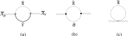
FIG. 1.: One-loop corrections to the two-point function $\overline{\cal A}_{\mu}$-$\overline{\cal A}_{\nu}$. The vertex with a dot ($\bullet$) implies the derivatives acting on the quantum fields, while that with a circle ($\circ$) implies no derivatives are included: The vertices in (a) are from $\Sigma^{(\pi V_{\beta})}_{ab}$ and $\Sigma^{(V_{\alpha}\pi)}_{ab}$ in Eqs. (B40) and (B41); the vertices in (b) are from $\Gamma^{(\pi\sigma)}_{\mu,ab}$ and $\Gamma^{(\sigma\pi)}_{\mu,ab}$ in Eqs. (B26) and (B27) together with the derivatives acting on the quantum fields; the vertex in (c) is from the first term of $\Sigma^{(\pi\pi)}_{ab}$ in Eq. (B32) and $\sum_{c}\Gamma^{(\pi\sigma)}_{\mu,ac}\Gamma^{\mu,(\sigma\pi)}_{cb}$ [32].

Let us start from the one-loop corrections to the two-point function $\overline{\cal A}_{\mu}$-$\overline{\cal A}_{\nu}$. The relevant diagrams are shown in Fig. 1. The divergent contributions of these diagrams are evaluated as

$$\left.\Pi_{\overline{\cal A}\overline{\cal A}}^{{\rm(a)}\mu\nu}(p)\right|_{\rm div}=g^{\mu\nu}\,\frac{N_{f}}{2(4\pi)^{2}}\left[-2a\bar{M}_{V}^{2}\,\ln\Lambda^{2}\right]\ ,$$ (C3)

$$\left.\Pi_{\overline{\cal A}\overline{\cal A}}^{{\rm(b)}\mu\nu}(p)\right|_{\rm div}=g^{\mu\nu}\,\frac{N_{f}}{2(4\pi)^{2}}\left[-a\Lambda^{2}+\frac{1}{2}a\bar{M}_{V}^{2}\,\ln\Lambda^{2}\right]$$ (C4)

$$\quad{}-\left(g^{\mu\nu}p^{2}-p^{\mu}p^{\nu}\right)\,\frac{N_{f}}{2(4\pi)^{2}}\frac{a}{6}\ln\Lambda^{2}\ ,$$ (C5)

$$\left.\Pi_{\overline{\cal A}\overline{\cal A}}^{{\rm(c)}\mu\nu}(p)\right|_{\rm div}=g^{\mu\nu}\,\frac{N_{f}}{2(4\pi)^{2}}\left[2(a-1)\Lambda^{2}\right]\ .$$ (C6)

The divergences in Eq. (C6) are renormalized by the bare parameters in the Lagrangian. The tree level contribution with the bare parameters is given by

$$\Pi_{\overline{\cal A}\overline{\cal A}}^{{\rm(tree)}\mu\nu}(p^{2})=F_{\pi,{\rm bare}}^{2}\,g^{\mu\nu}+2z_{2,{\rm bare}}\left(p^{2}g^{\mu\nu}-p^{\mu}p^{\nu}\right)\ .$$ (C7)

Thus the renormalization is done by requiring that the followings be finite:

$$F_{\pi,{\rm bare}}^{2}-\frac{N_{f}}{4(4\pi)^{2}}\left[2(2-a)\Lambda^{2}+3a^{2}g^{2}F_{\pi}^{2}\ln\Lambda^{2}\right]$$ (C8)

$$\qquad\qquad=\mbox{(finite)}\ ,$$ (C9)

$$z_{2,{\rm bare}}-\frac{N_{f}}{2(4\pi)^{2}}\,\frac{a}{12}\ln\Lambda^{2}=\mbox{(finite)}\ .$$ (C10)

The above renormalizations lead to the following RGE’s for $F_{\pi}$ [the first equation in Eqs. (9)] and $z_{2}$ [the second equation in Eqs. (14)]:

$$\mu\frac{dF_{\pi}^{2}}{d\mu}=\frac{N_{f}}{2(4\pi)^{2}}\left[3a^{2}g^{2}F_{\pi}^{2}+2(2-a)\mu^{2}\right]\ ,$$ (C11)

$$\mu\frac{dz_{2}}{d\mu}=\frac{N_{f}}{(4\pi)^{2}}\frac{a}{12}\ ,$$ (C12)

where $\mu$ is the renormalization scale.

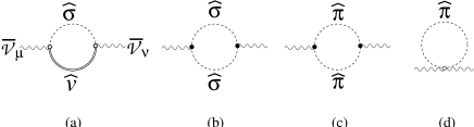
FIG. 2.: One-loop corrections to the two-point function $\overline{\cal V}_{\mu}$-$\overline{\cal V}_{\nu}$. The vertices in (a) are from $\Sigma^{(\sigma V_{\beta})}_{ab}$ and $\Sigma^{(V_{\alpha}\sigma)}_{ab}$ in Eqs. (B42) and (B43); the vertices in (b) are from $\Gamma^{(\sigma\sigma)}_{\mu,ab}$ in Eq. (B25) together with derivatives acting on the quantum fields; the vertices in (c) are from $\Gamma^{(\pi\pi)}_{\mu,ab}$ in Eq. (B24) together with derivatives acting on the quantum fields; the vertex in (d) is from the second term of $\Sigma^{(\pi\pi)}_{ab}$ in Eq. (B32) and $\sum_{c}\Gamma^{(\pi\pi)}_{\mu,ac}\Gamma^{\mu,(\pi\pi)}_{cb}$.

Next we calculate one-loop corrections to the two-point function $\overline{\cal V}_{\mu}$-$\overline{\cal V}_{\nu}$. The relevant diagrams are shown in Fig. 2. The divergent contributions are evaluated as

$$\left.\Pi_{\overline{\cal V}\overline{\cal V}}^{{\rm(a)}\mu\nu}(p)\right|_{\rm div}=g^{\mu\nu}\,\frac{N_{f}}{2(4\pi)^{2}}\left[-2a\bar{M}_{V}^{2}\,\ln\Lambda^{2}\right]\ ,$$ (C13)

$$\left.\Pi_{\overline{\cal V}\overline{\cal V}}^{{\rm(b)}\mu\nu}(p)\right|_{\rm div}=g^{\mu\nu}\,\frac{N_{f}}{2(4\pi)^{2}}\left[-\frac{1}{2}\Lambda^{2}+\frac{1}{2}\bar{M}_{V}^{2}\,\ln\Lambda^{2}\right]$$ (C14)

$$\quad{}-\left(g^{\mu\nu}p^{2}-p^{\mu}p^{\nu}\right)\,\frac{N_{f}}{2(4\pi)^{2}}\frac{1}{12}\ln\Lambda^{2}\ ,$$ (C15)

$$\left.\Pi_{\overline{\cal V}\overline{\cal V}}^{{\rm(c)}\mu\nu}(p)\right|_{\rm div}=g^{\mu\nu}\,\frac{N_{f}}{2(4\pi)^{2}}\left[-\frac{(2-a)^{2}}{2}\Lambda^{2}\right]$$ (C16)

$$\quad{}-\left(g^{\mu\nu}p^{2}-p^{\mu}p^{\nu}\right)\,\frac{N_{f}}{2(4\pi)^{2}}\frac{(2-a)^{2}}{12}\ln\Lambda^{2}\ ,$$ (C17)

$$\left.\Pi_{\overline{\cal V}\overline{\cal V}}^{{\rm(d)}\mu\nu}(p)\right|_{\rm div}=g^{\mu\nu}\,\frac{N_{f}}{2(4\pi)^{2}}\left[-2(a-1)\Lambda^{2}\right]\ .$$ (C18)

Similarly to the $\overline{\cal A}_{\mu}$-$\overline{\cal A}_{\nu}$ two-point function, we require that the following quantities be finite:

$$F_{\sigma,{\rm bare}}^{2}-\frac{N_{f}}{4(4\pi)^{2}}\left[(1+a^{2})\Lambda^{2}+3ag^{2}F_{\pi}^{2}\ln\Lambda^{2}\right]$$ (C19)

$$\qquad\qquad=\mbox{(finite)}\ ,$$ (C20)

$$z_{1,{\rm bare}}-\frac{N_{f}}{2(4\pi)^{2}}\,\frac{5-4a+a^{2}}{12}\ln\Lambda^{2}=\mbox{(finite)}\ .$$ (C21)

The above renormalizations lead to the following RGE’s for $F_{\sigma}$ and $z_{1}$ [the first equation in Eqs. (14)]:

$$\mu\frac{dF_{\sigma}^{2}}{d\mu}=\frac{N_{f}}{2(4\pi)^{2}}\left[3ag^{2}F_{\pi}^{2}+(1+a^{2})\mu^{2}\right]\ ,$$ (C22)

$$\mu\frac{dz_{1}}{d\mu}=\frac{N_{f}}{(4\pi)^{2}}\frac{5-4a+a^{2}}{24}\ .$$ (C23)

The RGE for $a\equiv F_{\sigma}^{2}/F_{\pi}^{2}$ [the second equation in Eqs. (9)] is derived from the RGE’s for $F_{\sigma}$ and $F_{\pi}$ given in Eqs. (C11) and (C22):

$$\mu\frac{da}{d\mu}=-C(a-1)\left[3a(a+1)g^{2}-(3a-1)\frac{\mu^{2}}{F_{\pi}^{2}}\right]\ ,$$ (C24)

where $C=N_{f}/[2(4\pi)^{2}]$.

Now, we calculate the one-loop correction to the two-point function $\overline{V}_{\mu}$-$\overline{V}_{\nu}$. The relevant diagrams are shown in Fig. 3. These are evaluated as

$$\left.\Pi_{\overline{V}\overline{V}}^{{\rm(a)}\mu\nu}(p)\right|_{\rm div}=g^{\mu\nu}\,\frac{N_{f}}{2(4\pi)^{2}}\left[-4\Lambda^{2}+8\bar{M}_{V}^{2}\,\ln\Lambda^{2}\right]$$ (C25)

$$\quad{}+\left(g^{\mu\nu}p^{2}-p^{\mu}p^{\nu}\right)\,\frac{N_{f}}{2(4\pi)^{2}}\frac{20}{3}\ln\Lambda^{2}\ ,$$ (C26)

$$\left.\Pi_{\overline{V}\overline{V}}^{{\rm(b)}\mu\nu}(p)\right|_{\rm div}=g^{\mu\nu}\,\frac{N_{f}}{2(4\pi)^{2}}\left[-2\bar{M}_{V}^{2}\,\ln\Lambda^{2}\right]\ ,$$ (C27)

$$\left.\Pi_{\overline{V}\overline{V}}^{{\rm(c)}\mu\nu}(p)\right|_{\rm div}=g^{\mu\nu}\,\frac{N_{f}}{2(4\pi)^{2}}\left[4\Lambda^{2}-4\bar{M}_{V}^{2}\,\ln\Lambda^{2}\right]$$ (C28)

$$\quad{}+\left(g^{\mu\nu}p^{2}-p^{\mu}p^{\nu}\right)\,\frac{N_{f}}{2(4\pi)^{2}}\frac{2}{3}\ln\Lambda^{2}\ ,$$ (C29)

$$\left.\Pi_{\overline{V}\overline{V}}^{{\rm(d)}\mu\nu}(p)\right|_{\rm div}=g^{\mu\nu}\,\frac{N_{f}}{2(4\pi)^{2}}\left[4\Lambda^{2}-8\bar{M}_{V}^{2}\,\ln\Lambda^{2}\right]\ ,$$ (C30)

$$\left.\Pi_{\overline{V}\overline{V}}^{{\rm(e)}\mu\nu}(p)\right|_{\rm div}=g^{\mu\nu}\,\frac{N_{f}}{2(4\pi)^{2}}\left[-4\Lambda^{2}+4\bar{M}_{V}^{2}\,\ln\Lambda^{2}\right]\ ,$$ (C31)

$$\left.\Pi_{\overline{V}\overline{V}}^{{\rm(f)}\mu\nu}(p)\right|_{\rm div}=g^{\mu\nu}\,\frac{N_{f}}{2(4\pi)^{2}}\left[-\frac{1}{2}\Lambda^{2}+\frac{1}{2}\bar{M}_{V}^{2}\,\ln\Lambda^{2}\right]$$ (C32)

$$\quad{}-\left(g^{\mu\nu}p^{2}-p^{\mu}p^{\nu}\right)\,\frac{N_{f}}{2(4\pi)^{2}}\frac{1}{12}\ln\Lambda^{2}$$ (C33)

$$\left.\Pi_{\overline{V}\overline{V}}^{{\rm(g)}\mu\nu}(p)\right|_{\rm div}=g^{\mu\nu}\,\frac{N_{f}}{2(4\pi)^{2}}\left[-\frac{a^{2}}{2}\Lambda^{2}\right]$$ (C34)

$$\quad{}-\left(g^{\mu\nu}p^{2}-p^{\mu}p^{\nu}\right)\,\frac{N_{f}}{2(4\pi)^{2}}\frac{a^{2}}{12}\ln\Lambda^{2}\ .$$ (C35)

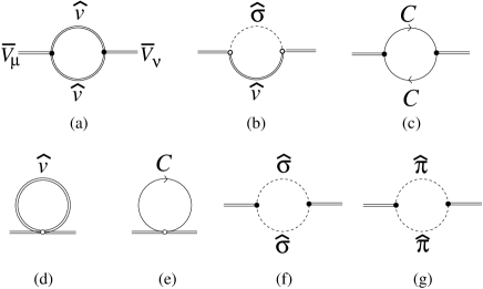
FIG. 3.: One-loop corrections to the two-point function $\overline{V}_{\mu}$-$\overline{V}_{\nu}$. The vertices in (a) are from $\Sigma^{(V_{\alpha}V_{\beta})}_{ab}$ in Eq. (B39) and $\Gamma^{(V_{\alpha}V_{\beta})}_{\mu,ab}$ in Eq. (B28) together with derivatives acting on the quantum fields; the vertices in (b) are from $\Sigma^{(\sigma V_{\beta})}_{ab}$ and $\Sigma^{(V_{\alpha}\sigma)}_{ab}$ in Eqs. (B42) and (B43); the vertices in (c) are from $\Gamma^{(CC)}_{\mu,ab}$ in Eq. (B74) together with derivatives acting on the quantum fields; the vertex in (d) is from $\Sigma^{(V_{\alpha}V_{\beta})}_{ab}$ and $\sum_{c,\gamma}\Gamma^{(V_{\alpha}}_{\mu,V_{\gamma}),ac}{\Gamma^{\mu,(V_{\gamma}V_{\beta})}_{cb}}$; the vertex in (e) is from $\sum_{c}\Gamma^{(CC)}_{\mu,ac}\Gamma^{\mu,(CC)}_{cb}$; the vertices in (f) are from $\Gamma^{(\sigma\sigma)}_{\mu,ab}$ in Eq. (B25) together with derivatives acting on the quantum fields; the vertices in (g) are from $\Gamma^{(\pi\pi)}_{\mu,ab}$ in Eq. (B24) together with derivatives acting on the quantum fields.

Summing up the contributions in Eq. (C35), we obtain the following divergent contribution:

$$\left.\Pi_{\overline{V}\overline{V}}^{{\mbox{(1-loop)}}\mu\nu}(p)\right|_{\rm div}$$ (C36)

$$\quad=-\frac{N_{f}}{4(4\pi)^{2}}\left[(1+a^{2})\Lambda^{2}+3ag^{2}F_{\pi}^{2}\ln\Lambda^{2}\right]g^{\mu\nu}$$ (C37)

$$\qquad{}+\frac{N_{f}}{2(4\pi)^{2}}\,\frac{87-a^{2}}{12}\ln\Lambda^{2}\left(p^{2}g^{\mu\nu}-p^{\mu}p^{\nu}\right)\ .$$ (C38)

On the other hand, the tree contribution is given by

$$\Pi_{\overline{V}\overline{V}}^{{\rm(tree)}\mu\nu}(p^{2})=F_{\sigma,{\rm bare}}^{2}\,g^{\mu\nu}-\frac{1}{g^{2}_{\rm bare}}\left(p^{2}g^{\mu\nu}-p^{\mu}p^{\nu}\right)\ .$$ (C39)

The first term in Eq. (C38) which is proportional to $g^{\mu\nu}$ is renormalized by $F_{\sigma,{\rm bare}}^{2}$ through the requirement in Eq. (C21). The second term in Eq. (C38) is renormalized by $g_{\rm bare}$ through

$$\frac{1}{g^{2}_{\rm bare}}-\frac{N_{f}}{2(4\pi)^{2}}\,\frac{87-a^{2}}{12}\ln\Lambda^{2}=\mbox{(finite)}\ .$$ (C40)

This renormalization leads to the following RGE for $g$ [the third equation in Eqs. (9)]:

$$\mu\frac{dg^{2}}{d\mu}=-\frac{N_{f}}{2(4\pi)^{2}}\frac{87-a^{2}}{6}g^{4}\ .$$ (C41)

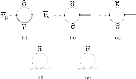
FIG. 4.: One-loop corrections to the two-point function $\overline{\cal V}_{\mu}$-$\overline{V}_{\nu}$. The vertices in (a) are from $\Sigma^{(\sigma V_{\beta})}_{ab}$ and $\Sigma^{(V_{\alpha}\sigma)}_{ab}$ in Eqs. (B42) and (B43); the vertices in (b) are from $\Gamma^{(\sigma\sigma)}_{\mu,ab}$ in Eq. (B25) together with derivatives acting on the quantum fields; the vertices in (c) are from $\Gamma^{(\pi\pi)}_{\mu,ab}$ in Eq. (B24) together with derivatives acting on the quantum fields; the vertex in (d) is from the second term of $\Sigma^{(\pi\pi)}_{ab}$ in Eq. (B32) and $\sum_{c}\Gamma^{(\pi\pi)}_{\mu,ac}\Gamma^{\mu,(\pi\pi)}_{cb}$; the vertex in (e) is from the second term of $\Sigma^{(\sigma\sigma)}_{ab}$ in Eq. (B34) and $\sum_{c}\Gamma^{(\sigma\sigma)}_{\mu,ac}\Gamma^{\mu,(\sigma\sigma)}_{cb}$.

We also calculate the one-loop correction to the two-point function $\overline{\cal V}_{\mu}$-$\overline{V}_{\nu}$ to determine the renormalization of $z_{3}$. The relevant diagrams are shown in Fig. 4. The divergent contributions are evaluated as

$$\left.\Pi_{\overline{\cal V}\overline{V}}^{{\rm(a)}\mu\nu}(p)\right|_{\rm div}=g^{\mu\nu}\,\frac{N_{f}}{2(4\pi)^{2}}\left[2\bar{M}_{V}^{2}\,\ln\Lambda^{2}\right]\ ,$$ (C42)

$$\left.\Pi_{\overline{\cal V}\overline{V}}^{{\rm(b)}\mu\nu}(p)\right|_{\rm div}=g^{\mu\nu}\,\frac{N_{f}}{2(4\pi)^{2}}\left[-\frac{1}{2}\Lambda^{2}+\frac{1}{2}\bar{M}_{V}^{2}\,\ln\Lambda^{2}\right]$$ (C43)

$$\quad{}-\left(g^{\mu\nu}p^{2}-p^{\mu}p^{\nu}\right)\,\frac{N_{f}}{2(4\pi)^{2}}\frac{1}{12}\ln\Lambda^{2}\ ,$$ (C44)

$$\left.\Pi_{\overline{\cal V}\overline{V}}^{{\rm(c)}\mu\nu}(p)\right|_{\rm div}=-g^{\mu\nu}\,\frac{N_{f}}{2(4\pi)^{2}}\,\frac{a(2-a)}{2}\Lambda^{2}$$ (C45)

$$\quad{}-\left(g^{\mu\nu}p^{2}-p^{\mu}p^{\nu}\right)\,\frac{N_{f}}{2(4\pi)^{2}}\frac{a(2-a)}{12}\ln\Lambda^{2}\ ,$$ (C46)

$$\left.\Pi_{\overline{\cal V}\overline{V}}^{{\rm(d)}\mu\nu}(p)\right|_{\rm div}=g^{\mu\nu}\,\frac{N_{f}}{2(4\pi)^{2}}a\Lambda^{2}\ ,$$ (C47)

$$\left.\Pi_{\overline{\cal V}\overline{V}}^{{\rm(e)}\mu\nu}(p)\right|_{\rm div}=g^{\mu\nu}\,\frac{N_{f}}{2(4\pi)^{2}}\left[\Lambda^{2}-2\bar{M}_{V}^{2}\,\ln\Lambda^{2}\right]\ .$$ (C48)

Thus

$$\left.\Pi_{\overline{\cal V}\overline{V}}^{{\mbox{(1-loop)}}\mu\nu}(p)\right|_{\rm div}$$ (C49)

$$\quad=\frac{N_{f}}{4(4\pi)^{2}}\left[(1+a^{2})\Lambda^{2}+3ag^{2}F_{\pi}^{2}\ln\Lambda^{2}\right]g^{\mu\nu}$$ (C50)

$$\qquad{}-\frac{N_{f}}{2(4\pi)^{2}}\,\frac{1+2a-a^{2}}{12}\ln\Lambda^{2}\left(p^{2}g^{\mu\nu}-p^{\mu}p^{\nu}\right)\ .$$ (C51)

The tree contribution is given by

$$\Pi_{\overline{\cal V}\overline{V}}^{{\rm(tree)}\mu\nu}(p^{2})=F_{\sigma,{\rm bare}}^{2}\,g^{\mu\nu}+2z_{3,{\rm bare}}\left(p^{2}g^{\mu\nu}-p^{\mu}p^{\nu}\right)\ .$$ (C52)

The first term in Eq. (C51) which is proportional to $g^{\mu\nu}$ is renormalized by $F_{\sigma,{\rm bare}}^{2}$ through the requirement in Eq. (C21). The second term in Eq. (C51) is renormalized by $z_{3,{\rm bare}}$ through

$$z_{3,{\rm bare}}-\frac{N_{f}}{2(4\pi)^{2}}\,\frac{1+2a-a^{2}}{12}\ln\Lambda^{2}=\mbox{(finite)}\ .$$ (C53)

This leads to [the third equation in Eqs. (14)]

$$\mu\frac{dz_{3}}{d\mu}=\frac{N_{f}}{(4\pi)^{2}}\frac{1+2a-a^{2}}{12}\ .$$ (C54)

To summarize, Eqs. (C11), (C24) and (C41) are the RGE’s for $F_{\pi}^{2}$, $a$ and $g$ shown in Eq. (9), and Eqs. (C23), (C12) and (C54) are the RGE’s for $z_{1}$, $z_{2}$ and $z_{3}$ shown in Eq. (14).

Below the $m_{\rho}$ scale, $\rho$ decouples and hence $F_{\pi}$ runs by the loop effect of $\pi$ alone. The relevant Lagrangian with least derivatives is given by the first term of Eq. (A68) [or equivalently, the first term of Eq. (5)], and the diagram contributing to $F_{\pi}^{2}$ is shown in Fig. 1(c). The resultant RGE for $F_{\pi}$ is given by

$$\mu\frac{d}{d\mu}\left[F_{\pi}^{(\pi)}\right]^{2}=\frac{2N_{f}}{(4\pi)^{2}}\mu^{2}\qquad(\mu<m_{\rho})\ .$$ (C55)

Unlike the parameters renormalized in a mass independent scheme, the parameter $F_{\pi}(\mu)$ ($\mu<m_{\rho}$) does not smoothly connect to $F_{\pi}(\mu)$ ($\mu>m_{\rho}$) at the $m_{\rho}$ scale. We need to include the effect of finite renormalization. This is evaluated by taking quadratic divergence proportional to $a$ in Eq. (C6) and replacing $\Lambda$ by $m_{\rho}$. This leads to the relation (34):

$$\left[F_{\pi}^{(\pi)}(m_{\rho})\right]^{2}=F_{\pi}^{2}(m_{\rho})+\frac{N_{f}}{(4\pi)^{2}}\frac{a(m_{\rho})}{2}m_{\rho}^{2}\ ,$$ (C56)

where $F_{\pi}^{(\pi)}(\mu)$ runs by the loop effect of $\pi$ alone for $\mu<m_{\rho}$.

Finally, let us show the finite correction to the relation for $L_{10}$ given in Eq. (37). This is evaluated from the finite part of the $g^{\mu\nu}$ part of the $\overline{\cal A}_{\mu}$-$\overline{\cal A}_{\nu}$ two-point function. [Here the $g^{\mu\nu}$ part of the $\overline{\cal A}_{\mu}$-$\overline{\cal A}_{\nu}$ two-point function is defined by $\Pi_{\overline{\cal A}\overline{\cal A}}^{L}(p^{2})\equiv\frac{p_{\mu}p_{\nu}}{p^{2}}\Pi_{\overline{\cal A}\overline{\cal A}}^{\mu\nu}(p)$.] From Fig. 1 we obtain

$$\Pi_{\overline{\cal A}\overline{\cal A}}^{(a)L}(p)=-N_{f}a\bar{M}_{v}^{2}B_{0}(p^{2};\bar{M}_{v},0)\ ,$$ (C57)

$$\Pi_{\overline{\cal A}\overline{\cal A}}^{(b)L}(p)=N_{f}\frac{a}{4}\left[B_{A}(p^{2};\bar{M}_{v},0)-A_{0}(\bar{M}_{v})-A_{0}(0)\right]\ ,$$ (C58)

$$\Pi_{\overline{\cal A}\overline{\cal A}}^{(c)L}(p)=N_{f}(a-1)A_{0}(0)\ ,$$ (C59)

where

$$A_{0}(M^{2})\equiv\int\frac{d^{n}k}{i(2\pi)^{n}}\frac{1}{M^{2}-k^{2}}\ ,$$ (C60)

$$B_{0}(p^{2};M,m)\equiv\int\frac{d^{n}k}{i(2\pi)^{n}}\frac{1}{[M^{2}-k^{2}][m^{2}-(k-p)^{2}]}\ ,$$ (C61)

$$B_{A}(p^{2};M,m)\equiv$$ (C62)

$$\quad\frac{(M^{2}-m^{2})^{2}}{p^{2}}\left[B_{0}(p^{2};M,m)-B_{0}(0;M,m)\right]\ .$$ (C63)

According to the analysis in Ref. [11], the ${\cal O}(p^{2})$ part of $\Pi_{\overline{\cal A}\overline{\cal A}}^{{\mbox{(1-loop)}}L}(p^{2})\equiv\Pi_{\overline{\cal A}\overline{\cal A}}^{(a)L}(p^{2})+\Pi_{\overline{\cal A}\overline{\cal A}}^{(b)L}(p^{2})+\Pi_{\overline{\cal A}\overline{\cal A}}^{(c)L}(p^{2})$ gives a finite order correction to $L_{10}$ as

$$-\frac{1}{4}\left.\frac{d}{dp^{2}}\Pi_{\overline{\cal A}\overline{\cal A}}^{{\mbox{(1-loop)}}L}(p^{2})\right|_{p^{2}=0}=\frac{N_{f}}{(4\pi)^{2}}\frac{11a}{96}\ ,$$ (C64)

which is the last term in Eq. (37).