Lepton asymmetries from neutrino oscillations

Abstract

Reasonably large relic neutrino asymmetries can be generated by active-sterile neutrino oscillations. After briefly discussing possible applications, I describe the Quantum Kinetic Equation formalism used to compute the asymmetry growth curves. I then show how the basic features of these curves can be understood on the basis of the adiabatic limit approximation in the collision dominated epoch, and the pure MSW effect at lower temperatures.

1 BRIEF OVERVIEW

The $\alpha$ flavour relic neutrino asymmetry $L_{\nu_{\alpha}}$ is defined by

$$L_{\nu_{\alpha}}=\frac{n_{\nu_{\alpha}}-n_{\overline{\nu}_{\alpha}}}{n_{\gamma}}$$ (1)

where $n_{\psi}$ is the number density of species $\psi$, and $\alpha=e,\mu,\tau$. Reasonably large values for $L_{\nu_{\alpha}}$ will be generated by $\nu_{\alpha}\leftrightarrow\nu_{s}$ and $\overline{\nu}_{\alpha}\leftrightarrow\overline{\nu}_{s}$ oscillations (where $s$ denotes a sterile species), in the temperature range $1$ MeV to $10$’s of MeV, provided that $\Delta m^{2}<0$ and the vacuum mixing angle $\theta_{0}$ is small [1, 2, 3, 4]. (Note that $|\Delta m^{2}|$ must be sufficiently large to induce significant asymmetry growth prior to neutrino decoupling at $1$ MeV. We focus on this case.) By convention, $\Delta m^{2}<0$ means that the predominantly sterile mass eigenstate is lighter than the predominantly active eigenstate. The asymmetry growth is seeded by the $CP$ asymmetric background plasma (baryon/electron asymmetry), and it is driven by runaway positive feedback conditions that prevail for a short time below a critical temperature $T_{c}$. Figure 1 shows $|L_{\nu_{\alpha}}|$ evolution for three different vacuum oscillation parameter choices [4].

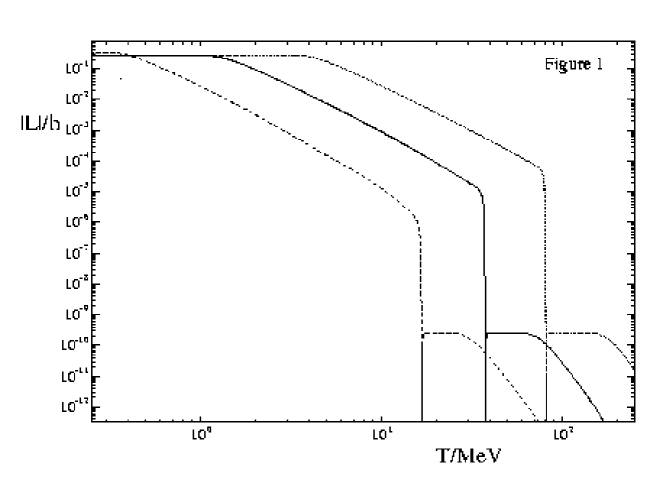
Figure 1: Examples of lepton asymmetry growth curves driven by $\nu_{\tau}\leftrightarrow\nu_{s}$ and the corresponding antineutrino oscillations. The mixing angle is selected to be $\sin^{2}2\theta=10^{-8}$. The three curves correspond to $\Delta m^{2}=-0.5,\ -50,\ -5000$ eV², reading left to right. This figure is taken from Ref.[4].

It is noteworthy that this mechanism requires light sterile neutrinos. These hypothetical degrees of freedom are interesting for other reasons also: as a simple explanation for two-fold maximal mixing (via the mirror matter [5] or pseudo-Dirac schemes [6]), and in order to reconcile the solar [7], atmospheric [8] and LSND anomalies [9].

Large neutrino asymmetries have found three potential applications. The first is the suppression of sterile neutrino production [1, 2, 4, 10]. Recall that the matter-affected mixing angle for neutrinos is given by

$$\sin^{2}2\theta_{m}=\frac{s^{2}}{s^{2}+(b-a-c)^{2}}$$ (2)

where $s\equiv\sin 2\theta_{0}$ and $c\equiv\cos 2\theta_{0}$. The functions $a$ and $b$ contribute to the effective potential [11]

$$V_{\alpha}=\frac{\Delta m^{2}}{2p}(-a+b)$$ (3)

where $p$ is the neutrino momentum or energy and

$$a = -\frac{2p\sqrt{2}G_{F}n_{\gamma}L}{\Delta m^{2}},$$

$$b = -\frac{2\sqrt{2}p^{2}\,G_{F}\,n_{\gamma}}{\Delta m^{2}}\frac{A_{\alpha}T}{m^{2}_{W}}.$$ (4)

The quantity $G_{F}$ is the Fermi constant, $m_{W}$ is the $W$ boson mass, $A_{e}\simeq 17$, $A_{\mu,\tau}\simeq 4.9$ and the effective total lepton number $L$ is

$$L\equiv L_{\nu_{\alpha}}+L_{\nu_{e}}+L_{\nu_{\mu}}+L_{\nu_{\tau}}+\eta,$$ (5)

where $|\eta|\sim 5\times 10^{-10}$ is a small term due to the asymmetry of the electrons and nucleons. The $a$ term is the Wolfenstein effective potential, while $b$ is a finite temperature correction that is very important in the early universe context. When $V_{\alpha}$ is large, the matter-affected mixing angle is small and sterile neutrino production is suppressed. At high $T$, the $b$ term alone is sufficient for this purpose, but at low $T$ a large enough $L$ is required.

The second application requires an electron-like asymmetry $L_{\nu_{e}}$ of the appropriate magnitude. Primordial light element abundances depend on the expansion rate of the universe during Big Bang Nucleosynthesis (BBN) as well as the reaction rates for $\overline{\nu}_{e}p\leftrightarrow e^{+}n$ and $\nu_{e}n\leftrightarrow e^{-}p$. The latter are affected by $L_{\nu_{e}}$, with a positive asymmetry lowering $n/p$ and thus also the Helium abundance. Now, the Helium yield increases with the baryon density $\eta_{B}$. A positive $L_{\nu_{e}}$ thus allows one to obtain an acceptable ⁴He mass fraction with a higher baryon density than would otherwise be the case [3, 12]. Interestingly, the recent Boomerang/Maxima cosmic microwave background anisotropy measurements prefer a relatively high $\eta_{B}$ [13]. This is a hint that $L_{\nu_{e}}>0$ should be taken seriously for phenomenological reasons.

The final application is related to the second. Recall that the effective potential depends on the linear combination $L$ which contains the baryon asymmetry $\eta$. Because of this, neutrino asymmetry generation depends on the properties of the baryonic component of the plasma. If the latter were to be spatially inhomogeneous, then it could seed inhomogeneous asymmetry creation [14]. There could be a domain structure, whereby the sign of $L_{\nu_{e}}$ flips between spatial cells. This will become especially interesting if future observations uncover firm evidence for inhomogeneous light element abundances.

Another interesting issue is the possibility of rapid oscillations in the asymmetry immediately after $T_{c}$ [1, 15, 16]. Recent work has shown that there are definitely no $L_{\nu_{\alpha}}$ oscillations for a large region of oscillation parameter space [16]. The remaining region requires significant computational effort, and has not been properly explored. There are indications for rapid oscillations, but numerical error cannot be definitively ruled out as their cause. On the theoretical front, it is strongly suspected that non-adiabatic effects should cause oscillations [2, 17], so it would not surprise if numerical work eventually confirms same (but only for a certain region of parameter space).

2 QUANTUM KINETIC EQUATIONS

The dynamical variable of interest is the 1-body reduced density matrix $\rho$ for the $\nu_{\alpha}/\nu_{s}$ subsystem. There is a corresponding density matrix for the antineutrinos. These functions depend on time $t$, or equivalently temperature $T$, and momentum $y\equiv p/T$. We will employ the decomposition

$$\rho\equiv\frac{1}{2}(P_{0}+\vec{P}\cdot\vec{\sigma}).$$ (6)

The diagonal entries are conveniently normalised distribution functions $f_{\alpha}$ and $f_{s}$ for $\nu_{\alpha}$ and $\nu_{s}$, respectively:

$$f_{\alpha}=\frac{1}{2}(P_{0}+P_{z})f_{eq}^{0},\quad f_{s}=\frac{1}{2}(P_{0}-P_{z})f_{eq}^{0}.$$ (7)

The off-diagonal entries $P_{x,y}$ are the coherences.

The Quantum Kinetic Equations (QKEs) are [18]

$${\partial\vec{P}\over\partial t}=\vec{V}\times\vec{P}-D(P_{x}{\bf\hat{x}}+P_{y}{\bf\hat{y}})+{\partial P_{0}\over\partial t}\,{\bf\hat{z}},$$ (8)

$${\partial P_{0}\over\partial t}\equiv R\simeq\Gamma(y)\left\{{f_{eq}\over f^{0}_{eq}}-{1\over 2}(P_{0}+P_{z})\right\}.$$ (9)

The damping or decoherence function $D$ is given by $D=\frac{\Gamma}{2}$, with $\Gamma$ being the total collision rate of the weak eigenstate neutrino of momentum $y$ with the background plasma, $\Gamma(y)\simeq\kappa_{\alpha}\,G_{F}^{2}T^{5}\,y$, where $\kappa_{e}\simeq 1.27$ and $\kappa_{\mu}=\kappa_{\tau}\simeq 0.92$ (for $m_{e}\stackrel{{\scriptstyle<}}{{\sim}}T\stackrel{{\scriptstyle<}}{{\sim}}m_{\mu}$).

The function $f_{eq}$ is the Fermi-Dirac distribution,

$$f_{eq}(y)\equiv{1\over 1+e^{y-\tilde{\mu}_{\alpha}}}.$$ (10)

where $\tilde{\mu}_{\alpha}\equiv\mu_{\nu_{\alpha}}/T$ is a dimensionless chemical potential, and $f^{0}_{eq}$ is the $\mu_{\nu_{\alpha}}=0$ case.

The quantity $\vec{V}$ is given by

$${\bf V}=\beta{\bf\hat{x}}+\lambda{\bf\hat{z}},$$ (11)

where

$$\beta=\frac{\sin 2\theta_{0}}{\ell_{0}},\quad\lambda=-\frac{\cos 2\theta_{0}}{\ell_{0}}+V_{\alpha},$$ (12)

and $\ell_{0}\equiv 2yT/\Delta m^{2}$ is the vacuum oscillation length.

The $\vec{V}\times\vec{P}$ term describes coherent nonlinear MSW evolution, the $D$ entry represents collisional decoherence, while $R$ quantifies repopulation of the $\nu_{\alpha}$ distribution from the background plasma.

An overbar will designate corresponding antineutrino functions. The kinetic equations are identical except for the substitution $L\to-L$.

The QKEs together with $\alpha+s$ lepton number conservation supply

$$\frac{dL_{\nu_{\alpha}}}{dt}=\frac{T^{3}}{2n_{\gamma}}\int_{0}^{\infty}\beta(P_{y}-\overline{P}_{y})\frac{y^{2}f_{eq}^{0}}{2\pi^{2}}dy$$ (13)

as the asymmetry evolution equation. This is a redundant equation, but numerically very useful in removing the problem of taking the difference of two large numbers to obtain the asymmetry. It is nonlinear, because $\lambda$ and $\overline{\lambda}$ depend on $L_{\nu_{\alpha}}$.

3 ANALYTICAL AND PHYSICAL UNDERSTANDING OF ASYMMETRY GROWTH

The growth curves in Fig.1 were obtained by numerically solving the QKEs in conjunction with Eq.(13). In this section I review how the QKE “black box” may be opened and the basic features of these graphs analytically and physically understood. This will provide a partial reply to the claims of Ref.[19]. A more complete riposte can be found in Ref.[20].

3.1 Collision dominated epoch

The collision rate $\Gamma$ is proportional to $T^{5}$, so at high enough temperatures collisions dominate the evolution. In this epoch it is legitimate to take $R\simeq 0$, because $f_{\alpha}$ does not depart from equilibrium form very strongly. See Ref.[21] for a discussion. The QKEs then reduce to

$${\partial{\bf P}\over\partial t}\simeq{\cal K}{\bf P}=\left(\begin{array}[]{ccc}-D&-\lambda&0\\ \lambda&-D&-\beta\\ 0&\beta&0\end{array}\right)\left(\begin{array}[]{c}P_{x}\\ P_{y}\\ P_{z}\end{array}\right).$$ (14)

In the instantaneous diagonal basis ${\bf Q}={\cal U}{\bf P}$ this equation becomes

$$\frac{\partial{\bf Q}}{\partial t}={\cal K}_{d}{\bf Q}-{\cal U}\frac{\partial{\cal U}^{-1}}{\partial t}{\bf Q},$$ (15)

where ${\cal K}_{d}$ is the diagonal matrix of eigenvalues $k_{1,2,3}$ of ${\cal K}$. In the adiabatic limit we set ${\partial{\cal U}^{-1}}/{\partial t}=0$ and Eq.(15) may be formally solved to yield [17, 22]

$${\bf P}(t)\simeq{\cal U}^{-1}(t)e^{\int_{0}^{t}{\cal K}_{d}dt^{\prime}}{\cal U}(0){\cal P}(0).$$ (16)

Under most circumstances, the eigenvalues take the form [17]

$$k_{1}=k_{2}^{*}=-d+i\omega,\quad k_{3}=-\frac{\beta^{2}D}{d^{2}+\omega^{2}},$$ (17)

with

$$d=D+\frac{k_{3}}{2},\quad\omega^{2}=\lambda^{2}+\beta^{2}+k_{3}D+\frac{3}{4}k_{3}^{2}.$$ (18)

In the high $T$ collision dominated regime

$$d\simeq D,\quad\omega\simeq\sqrt{\beta^{2}+\lambda^{2}}$$ (19)

and

$$k_{3}\simeq-\frac{\beta^{2}D}{D^{2}+\lambda^{2}+\beta^{2}}\ll D,$$ (20)

except at the very centre of the resonance. For full technical details concerning the resonance regime see Ref.[17]. When collisions dominate, $\exp(\int k_{1,2}dt^{\prime})\to 0$, and Eq.(16) yields

$$P_{y}(t)\simeq\frac{k_{3}}{\beta}P_{z}(t),$$ (21)

so that Eq.(13) becomes

$$\frac{dL_{\nu_{\alpha}}}{dt}=\frac{T^{3}}{2n_{\gamma}}\int_{0}^{\infty}(k_{3}P_{z}-\overline{k}_{3}\overline{P}_{z})\frac{y^{2}f_{eq}^{0}}{2\pi^{2}}dy.$$ (22)

One also obtains a sterile neutrino production equation which I will not display. These equations involve the distribution functions only – the coherences have been eliminated – so we have a Boltzmann limit. The root of this lies with the collisional damping by $-d$ of the oscillatory behaviour driven by $\omega$.

Substituting for the various functions on the righthand side of Eq.(22) one finally obtains, to leading order [1, 2, 22],

$$\frac{dL_{\nu_{\alpha}}}{dt}\simeq\frac{s^{2}T^{3}}{4\pi^{2}n_{\gamma}}\times$$

$$\int_{0}^{\infty}dy\frac{\Gamma a(c-b)(f_{\alpha}+f_{\overline{\alpha}}-f_{s}-f_{\overline{s}})y^{2}}{[x+(c-b+a)^{2}][x+(c-b-a)^{2}]},$$ (23)

where $x\equiv s^{2}+(D\ell_{0})^{2}$. This has been called the “static approximation”. There are correction terms also which I will not discuss. If $\Delta m^{2}>0$, then it is easy to see $dL_{\nu_{\alpha}}/dt\sim-L$ and so $L_{\nu_{\alpha}}$ evolves so as to drive the effective asymmetry $L$ to zero. The $\Delta m^{2}<0$ case is, however, quite different. The function $b$ is then always positive, decreasing as $T^{5}$, and the sign of the asymmetry derivative changes from negative to positive at a critical temperature $T_{c}$ due to the evolving net effect of the $(c-b)$ factor in the integrand. Immediately after $T_{c}$, a brief spurt of exponential growth occurs because now $dL_{\nu_{\alpha}}/dt\sim+L$.

The dashed line in Fig.2, taken from Ref.[3], shows the asymmetry growth curve obtain from Eq.(23). The dash-dotted curve displays asymmetry evolution as obtained from the full QKEs for the same oscillation parameter choice. The explosive growth at $T_{c}$ is well approximated by Eq.(23), demonstrating that collision dominated adiabatic evolution is the dominant physical effect during this epoch. At lower $T$, the magnitude of the asymmetry is seriously underestimated. New physics has taken over [3].

Figure 2: Asymmetry growth curves from the QKEs (dash-dotted line), the static approxmation (dashed line) and undamped adiabatic MSW transitions (solid line) as presented in Ref.[3] for $\Delta m^{2}=-10$ eV² and $\sin^{2}2\theta_{0}=10^{-9}$.

3.2 MSW dominated epoch

We begin by observing that Eq.(22) reduces to $dL_{\nu_{\alpha}}/dt=0$ when the collision rate $\Gamma$ vanishes. This helps to explain why the approximate evolution equation reviewed above underestimates asymmetry growth at lower temperatures. When collisions are unimportant, the QKEs describe pure (non-linear) matter-affected evolution, so we now turn to a study of the MSW effect.

Putting $D=\Gamma/2=0$ in the adiabatic evolution matrix ${\cal K}$ produces the eigenvalues

$$k_{1}=k_{2}^{*}=i\sqrt{\beta^{2}+\lambda^{2}},\quad k_{3}=0.$$ (24)

There is no damping so the evolution is oscillatory, with $|k_{1,2}|$ being the matter-affected oscillation frequency for a neutrino of momentum $y$. The conditions for the validity of Eqs.(22) and (23) no longer hold [17, 22].

Furthermore, the condition of the plasma is now different because of the significant neutrino asymmetry, leading to a separation of the neutrino and antineutrino resonance momenta $y^{r}$ [3]. Writing $a\equiv\xi_{a}y$ and $b\equiv\xi_{b}y^{2}$, the MSW resonance conditions $c-b\mp a=0$ imply that

$$y^{r}_{\nu}=\frac{\xi_{a}+\sqrt{\xi_{a}^{2}+4\xi_{b}}}{2\xi_{b}}$$ (25)

and

$$y^{r}_{\overline{\nu}}=\frac{-\xi_{a}+\sqrt{\xi_{a}^{2}+4\xi_{b}}}{2\xi_{b}}.$$ (26)

If $L>0$, then $\xi_{a}$ is positive and $y^{r}_{\nu}$ quickly moves to the high-momentum tail of the distribution. The partial cancellation between the terms in the numerator of $y^{r}_{\overline{\nu}}$ keeps the antineutrino resonance within the body of the distribution. Doing the algebra with $\xi_{b}\ll\xi_{a}$ one obtains

$$y^{r}_{\overline{\nu}}\simeq\frac{\pi^{2}|\Delta m^{2}|}{8\sqrt{2}\zeta(3)G_{F}}\frac{1}{L_{\nu_{\alpha}}T^{4}},$$ (27)

where we have taken $L\simeq 2L_{\nu_{\alpha}}$. The resonance momentum evolution [3] is shown in Fig.3.

Figure 3: The separation of the neutrino and antineutrino resonance momenta as the asymmetry grows. The oscillation parameters are as for Fig.2. This figure first appeared in Ref.[3].

The separation of the resonances means that the MSW effect has very asymmetric (pardon the pun) consequences for neutrinos and antineutrinos: neutrino oscillation are strongly suppressed, whereas $\overline{\nu}_{\alpha}$’s get MSW converted into sterile states. This keeps the positive $L$ growing [3]. (The final sign of $L$, but not its magnitude, depends on the high $T$ initial neutrino chemical potentials and so cannot be predicted.) The MSW effect is of course automatically taken care of by the QKEs. But in order to isolate its influence, a more physical approach is useful. We will stay with the $L>0$ case. For small resonance widths and $100\%$ (adiabatic) conversion, the rate of change of the asymmetry is proportional to the speed with which the antineutrino resonance moves through the distribution [3]:

$$\frac{dL_{\nu_{\alpha}}}{dT}=-\frac{T^{3}}{2\pi^{2}n_{\gamma}}\,[f_{\overline{\nu}_{\alpha}}(y^{r}_{\overline{\nu}})-f_{\overline{\nu}_{s}}(y^{r}_{\overline{\nu}})]\,(y^{r}_{\overline{\nu}})^{2}\,\frac{dy^{r}_{\overline{\nu}}}{dT}$$

$$\equiv-X\frac{dy^{r}_{\overline{\nu}}}{dT}$$ (28)

Using Eq. (27) one then obtains

$$\frac{dL_{\nu_{\alpha}}}{dT}=-\frac{4}{T}\frac{Xy^{r}_{\overline{\nu}}}{1+\frac{Xy^{r}_{\overline{\nu}}}{L_{\nu_{\alpha}}}}$$ (29)

as a non-linear evolution equation for the asymmetry, for the case where $\frac{dy^{r}_{\overline{\nu}}}{dT}<0$. We employ instantaneous repopulation before neutrino decoupling, so $f_{\overline{\alpha}}$ is understood to be of Fermi-Dirac form with the appropriate (evolving) chemical potential. After chemical and kinetic decoupling one has to handle repopulation in a more complicated way: see Refs.[3, 12] for further explanations.

The solid line in Fig.2 shows the result of numerically integrating Eq.(29), beginning at $T\simeq T_{c}/2$. The agreement with the QKE result is excellent, which shows that the MSW effect has taken over by $T\simeq T_{c}/2$ [3]. Furthermore, when $L_{\nu_{\alpha}}\ll 1$, Eq.(29) reduces to

$$\frac{dL_{\nu_{\alpha}}}{dT}\simeq-\frac{4L_{\nu_{\alpha}}}{T},$$ (30)

which immediately implies that $L_{\nu_{\alpha}}\sim T^{-4}$. The power law behaviour displayed by the QKE solution is thus easily understood as a consequence of undamped adiabatic MSW transitions [3].

As the asymmetry continues to grow, the antineutrino resonance eventually moves out of the body into the high momentum end of the distribution. The asymmetry becomes frozen at some final steady state value, whose approximate magnitude can be easily understood by integrating the Fermi–Dirac distribution from $y\sim 0$ to $y=\infty$ [3]:

$$L^{\rm final}_{\nu_{\alpha}}\sim\frac{1}{4\zeta(3)}\left(\frac{T_{\nu_{\alpha}}}{T_{\gamma}}\right)^{3}\int_{0}^{\infty}\frac{y^{2}dy}{1+e^{y}}$$

$$=\frac{3}{8}\left(\frac{T_{\nu_{\alpha}}}{T_{\gamma}}\right)^{3}.$$ (31)

The temperature ratio takes care of reheating due to $e^{+}e^{-}$ annihilations at $T\simeq m_{e}\simeq 0.5$ MeV. Equation (31) gives the approximate magnitude only, because the distribution changes with time as the asymmetry is created. Numerically, the final values found by incorporating proper thermalisation effects are quite close to this estimate.

4 CONCLUSIONS

Active-sterile neutrino oscillations will produce a final steady state asymmetry of order $3/8$ provided the oscillation parameters are in the appropriate range. Applications include the suppression of sterile neutrino production prior to BBN and the alteration of the primoridal Helium abundance due to a $\nu_{e}$ asymmetry. Inhomogeneous baryogenesis can seed lepton domain formation leading to inhomogeneous BBN. The asymmetry growth curves obtained from brute force numerical solution of the QKEs have been understood analytically and physically.

References

- [1] R. Foot, M. J. Thomson and R. R. Volkas, Phys. Rev. D 53 (1996) 5349.
- [2] R. Foot and R. R. Volkas, Phys. Rev. D 55 (1997) 5147.
- [3] R. Foot and R. R. Volkas, Phys. Rev. D56 (1997) 6653; Erratum, Phys. Rev. D59 (1999) 029901;
- [4] R. Foot, Astropart. Phys. 10 (1999) 253.
- [5] R. Foot, H. Lew and R. R. Volkas, Phys. Lett. B272 (1991) 67; Mod. Phys. Lett. A7 (1992) 2567; R. Foot, Mod. Phys. Lett. A9 (1994) 169; R. Foot and R. R. Volkas, Phys. Rev. D52 (1995) 6595; Astropart. Phys. 7 (1997) 283; Phys. Rev. D61 (2000) 043507.
- [6] S. M. Bilenky and S. T. Petcov, Rev. Mod. Phys. 59 (1987) 671; D. Chang and O. C. W. Kong, Phys. Lett. B477 (2000) 416; J. Bowes and R. R. Volkas, J. Phys. G24 (1998) 1249; A. Geiser, Phys. Lett. B444 (1999) 358; P. Langacker, Phys. Rev. D58 (1998) 093017; Y. Koide and H. Fusaoka, Phys. Rev. D59 (1999) 053004; C. Giunti, C. W. Kim and U. W. Kim, Phys. Rev. D46 (1992) 3034; M. Kobayashi, C. S. Lim and M. M. Nojiri, Phys. Rev. Lett. 67 (1991) 1685.
- [7] Y. Suzuki, these Proceedings.
- [8] H. Sobel, these Proceedings.
- [9] G. Mills, these Proceedings.
- [10] P. Di Bari, P. Lipari and M. Lusignoli, Int. J. Mod. Phys. A15 (2000) 2289.
- [11] L. Wolfenstein, Phys. Rev. D17 (1978) 2369; D20 (1979) 2634; S. P. Mikheyev and A. Yu. Smirnov, Nuovo Cimento C 9 (1986) 17; D. Nötzold and G. Raffelt, Nucl. Phys. B307 (1988) 924.
- [12] N. F. Bell, R. Foot and R. R. Volkas, Phys. Rev. D58 (1998) 105010.
- [13] P. de Bernardis et al., Nature 404 (2000) 955; A. E. Lange et al., astro-ph/0005004; S. Hanany et al., astro-ph/0005123; A. Balbi et al., astro-ph/0005124; see also, S. Esposito et al., astro-ph/0005571.
- [14] P. Di Bari, Phys. Lett. B482 (2000) 150.
- [15] X. Shi, Phys. Rev. D54 (1996) 2753; K. Enqvist, K. Kainulainen and A. Sorri, Phys. Lett. B464 (1999) 199; A. Sorri, Phys. Lett. B477 (2000) 201.
- [16] P. Di Bari and R. Foot, Phys. Rev. D61 (2000) 105012.
- [17] R. R. Volkas and Y. Y. Y. Wong, hep-ph/0007185, Phys. Rev. D (in press).
- [18] R. A. Harris and L. Stodolsky, Phys. Lett. 116B (1982) 464; B78 (1978) 313; A. Dolgov, Sov. J. Nucl. Phys. 33 (1981) 700; L. Stodolsky, Phys. Rev. D36 (1987) 2273; M. Thomson, Phys. Rev. A45 (1991) 2243; K. Enqvist, K. Kainulainen and J. Maalampi, Nucl. Phys. B349 (1991) 754; B. H. J. McKellar and M. J. Thomson, Phys. Rev. D49 (1994) 2710.
- [19] A. D. Dolgov, S. H. Hansen, S. Pastor and D. V. Semikoz, Astropart. Phys. 14 (2000) 79.
- [20] P. Di Bari, R. Foot, R. R. Volkas and Y. Y. Y. Wong, hep-ph/0008245.
- [21] K. S. M. Lee, R. R. Volkas and Y. Y. Y. Wong, hep-ph/0007186, Phys. Rev. D (in press).
- [22] N. F. Bell, R. R. Volkas and Y. Y. Y. Wong, Phys. Rev. D59 (1999) 113001.