Abstract

We use an optimised hopping parameter expansion for the free energy (linear $\delta$-expansion) to study the phase transitions at finite temperature and finite charge density in a global U(1) scalar Higgs sector on the lattice at large lattice couplings. We are able to plot out phase diagrams in lattice parameter space and find that the standard second-order phase transition with temperature at zero chemical potential becomes first order as the chemical potential increases.

1 Introduction

Quantum field theory has had many remarkable successes in the past fifty years using the standard methods of perturbative expansions. However, there are many situations where such techniques are not appropriate. The obvious example is QCD, which has strongly coupled bound states at low momenta. However, phase transitions at non-zero temperatures and densities, even in models without infrared slavery like the electroweak model, are also poorly explained by perturbative methods. It is this latter example which motivates our interest in scalar Higgs fields. The global U(1) model is also a relatively simple testing ground for techniques at finite chemical potential and temperature. There are many examples of physical situations at finite charge densities. Any phase transitions after baryogenesis in the early universe occur at finite baryon charge density. Heavy ion collisions also occur in the same regime.

Having ruled out a perturbative approach we turn to the various available non-perturbative techniques. One’s first thought is to use Monte Carlo (MC) techniques to tackle the problem. However, MC methods usually fail when considering models at finite densities. This is because the Euclidean action, which is used as a statistical weight for the system, becomes complex, making a simple statistical integration technique imposible.

To replace the MC approach we need an analytical non-perturbative method. The method chosen in this paper is an example of a general family sometimes called linear $\delta$-expansions [5]. Examples of these methods have appeared under many names, including optimised pertubation theory[4], action-variational approach [17], variational perturbation theory [21], method of self-similar approximations [22], screened perturbation theory [20],and the variational cumulant expansion [23]. The method has been applied successfully to the evaluation of simple integrals [5, 14, 15], solving non-linear differential equations [16], quantum mechanics [5, 13, 24, 25, 26], cosmological slow roll transitions [7] and to quantum field theory, both in the continuum [26, 21] and on the lattice [5, 8, 9, 10, 11, 12, 17, 18, 19, 23, 28, 29]. Since the LDE approach is analytical, we do not have to worry about the presence of a complex action. The expectation value of all physical observables will turn out to be real.

The work in this paper with the $U(1)$ or $O(2)$ model builds on that set out in [4] for the case of zero temperature and zero chemical potential. However, here we phrase the model in terms of the field and its conjugate $(\Phi,\Phi^{*})$ rather than working with the real components of the field. This change is made because the charge operator is diagonal in this representation and so much easier to deal with[32].

This paper is also complementary to the work done on the $U(1)$ model using LDE methods in the continuum at finite temperature and finite chemical potential [6].

2 The Linear Delta expansion

The general format of the LDE method is to take a given expansion, whether it be a perturbative expansion in the continuum or a cumulant expansion on the lattice, and to provide an order by order optimisation of this expansion. It is in this process of optimisation that non-perturbative information emerges. It is straightforward, in principle, to expand beyond leading order, unlike other non-perturbative methods like large-N expansions or mean-field approximations.

The first step in the method is to replace the physical action with an interpolating action made up of a linear combination of the physical action and a soluble trial action. This trial action is characterised by some set of new variational parameters $\{\vec{v}\}$. The particular choice of trial action is the main decision to be made in implementing the method. The more general the trial action, and the more terms one includes, the greater the number of variational parameters required to characterise it. The interpolating action takes the form $S\rightarrow S_{\delta}=S_{0}(\vec{v})+\delta(S-S_{0}(\vec{v}))$. If we set $\delta=1$ in the interpolating action then $S_{\delta}=S$. The new statistical average of an operator $O$ is

$$\left\langle O\right\rangle_{\delta}=\frac{1}{Z_{\delta}}\int{\cal D}\Phi\;O\;e^{-S_{0}}e^{\delta(S-S_{0})}$$ (1)

We now perform our chosen expansion technique on this new action. In this paper we use an expansion for the free energy on the lattice in terms of cumulant averages (sometimes known as a linked cluster expansion). However, we expand in the unphysical parameter $\delta$ instead of the coupling or the hopping parameter. The new expansion, as compared to the original, has additional terms at each order which depend upon the variational parameters. When we truncate the expansion at a given power of $\delta$ and then impose $\delta=1$ there remains a residual dependence on these varational parameters. So the LDE up to $\delta^{R}$ for the expectation value of some operator $\hat{\mathcal{O}}$ is

$$\left\langle\mathcal{O}\right\rangle_{R}=\left\langle\mathcal{O}\right\rangle_{R}\left(\vec{v}\right):=\lim_{\delta\rightarrow 1}\left\{\left\langle\mathcal{O}\right\rangle_{\delta}\left(\vec{v}\right)\right\}_{R}$$ (2)

where the $\{\}_{R}$ bracket signifies the truncation of the power series to order $\delta^{R}$. It is how we choose to fix the variational parameters, order by order in the expansion, which introduces the main fully non-perturbative effects. There are at least two apparently different approaches to this final part of the method listed in the literature. The first is to demand that the series converge as fast as possible by minimising the highest order term with respect to the lower order terms [17] - the principle of fastest convergence. However, we shall take the second main approach, often called the principle of minimal sensitivity (PMS)[30]. This is discussed in [5, 8, 9, 10] and used in standard partical physics to minimise dependence of perturbative results on the renormalisation scheme choice[31]. For the PMS case the parameters, $\{\vec{v}\}$, are set at each order in the expansion by demanding that the variation of some physical observable be zero. It is useful to be aware of the general statement that a derivative of (2) with respect to some arbitary parameter $x$ gives

$$\frac{\partial\left\langle\mathcal{O}\right\rangle_{R}}{\partial x}=\left\langle\frac{\partial\mathcal{O}}{\partial x}\right\rangle_{R} - \lim_{\delta\rightarrow 1}\left[\left\langle\frac{\partial S_{0}}{\partial x}\mathcal{O}\right\rangle_{\delta}-\left\langle\frac{\partial S_{0}}{\partial x}\right\rangle_{\delta}\left\langle\mathcal{O}\right\rangle_{\delta}\right]_{\rm R^{\it th}\,term}$$ (3)

$$- \lim_{\delta\rightarrow 1}\left\{\left\langle\frac{\partial S}{\partial x}\mathcal{O}\right\rangle_{\delta}-\left\langle\frac{\partial S}{\partial x}\right\rangle_{\delta}\left\langle\mathcal{O}\right\rangle_{\delta}\right\}_{R-1}$$

The first term is just an LDE up to order $R$, the second is just the last term in an LDE expansion up to order $R$ and the final term is an LDE up to order $R-1$. This means that the PMS condition on a variational parameter is

$$\frac{\partial\left\langle\mathcal{O}\right\rangle_{R}}{\partial v}=0\Longrightarrow\lim_{\delta\rightarrow 1}\left[\left\langle\frac{\partial S_{0}}{\partial v}\mathcal{O}\right\rangle_{\delta}-\left\langle\frac{\partial S_{0}}{\partial x}\right\rangle_{\delta}\left\langle\mathcal{O}\right\rangle_{\delta}\right]_{\rm R^{th}term}=0$$ (4)

In the special case of the free energy, defined by $F=-(1/N)\ln Z$, we have instead

$$\frac{\partial F_{R}}{\partial x}=\frac{1}{N}\lim_{\delta\rightarrow 1}\left[\left\langle\frac{\partial S_{0}}{\partial x}\right\rangle_{\delta}\right]_{\rm R^{th}term}+\frac{1}{N}\lim_{\delta\rightarrow 1}\left\{\left\langle\frac{\partial S}{\partial x}\right\rangle_{\delta}\right\}_{R-1}$$ (5)

$$\frac{\partial F_{R}}{\partial v}=0\Longrightarrow\lim_{\delta\rightarrow 1}\left[\left\langle\frac{\partial S_{0}}{\partial v}\right\rangle_{\delta}\right]_{\rm R^{th}term}=0$$ (6)

In general the PMS condition is only a condition on the final term in the expansion. In this way one sees that the PMS and principle of fastest convergence are quite closely related.

The variational parameters are set order by order by (4) or (6) and then substituted back into the expression for the physical observable to obtain the LDE estimate for its value. In quantum mechanical models at least, the absolute convergence of this LDE estimate to the true solution can be proven[13].

We have set out the two overall approaches to fixing the varational parameters. However, the choice of what physical observable one chooses for the PMS procedure vastly increases the possible options. One can for example always apply the PMS techniques to an LDE for the particular observable one is trying to measure; this could be called a true PMS approach. On the other hand one could choose to extremise an LDE for one particular physical observable, say the free energy, and then apply the values of the variational parameters gleaned therefrom to another LDE for the particular physical observable one is interested in. These two options are discussedin [4] for the $O(2)$ scalar model and the second option is preferred.

We have set out the two overall approaches to fixing the variational parameters. However, there is a further degree of freedom in the choice of which physical observable to apply the PMS procedure to. The strict LDE approach would be to apply the PMS procedure to the expansion for the observable one is interested in. However, in some cases (see, for example, Ref. 4 for the $O(2)$ scalar model) there may be no PMS points in that expansion. The alternative is to fix the variational parameters by applying the PMS procedure to the expansion for one particular, privileged observable, e.g. the free energy, and then use those parameters in the expansions for all other observables.

In this paper we shall take what is effectively the second approach, but instead of calculating two expansions, one for the free energy and one for the physical parameter we are trying to evaluate, we will evaluate the free energy using an LDE approach with the PMS criterion and then calculate all the other required physical observables by numerical differentiation with respect to the physical parameters of the free energy.

3 The U(1) complex scalar model on the lattice

We work with a Euclidean time formulation of the $U(1)$ field theory. In the continuum the global U(1) model at finite density has a conserved charge of the form ${\cal Q}=i(\Phi^{*}\Pi-\Phi\Pi^{*})$. The presence of a finite charge density at finite temperature gives rise to an effective action[32]

$$S_{\rm eff}=-\int_{0}^{\beta}dt\int d^{3}x\left[(\nabla_{\mu}\Phi)^{*}(\nabla^{\mu}\Phi)+(\mu_{0}^{2}-m_{0}^{2})\Phi^{*}\Phi-\lambda_{0}(\Phi^{*}\Phi)^{2}\right.$$

$$\left.-i\mu_{0}(\Phi^{*}\dot{\Phi}-\Phi\dot{\Phi^{*}})+J_{0}^{*}\Phi+J_{0}\Phi^{*}\right]$$ (7)

The temperature appears as a finite boundary condition in the Euclidean time direction, where $N_{t}a_{t}=1/T$. The integer $N_{t}$ is the number of lattice links in the temporal direction and $a_{t}$ is the temporal lattice spacing. In contrast the chemical potential is present in the main body of the Lagrangian. In particular we have a slightly surprising $\mu_{0}^{2}$ term which arises from integrating out the conjugate fields when constructing the effective action. This term can cause symmetry breaking with positive $m_{0}^{2}$, even for free fields, when the transition occurs at $\mu=m_{L}$. In a Euclidean formulation the effective action is complex. This complexification caused by the introduction of a chemical potential is generic. In addition, the presence of the chemical potential means that the action is not invariant under $t\rightarrow-t$ (Osterwalder-Schrader reflection)[1].

To regularise the UV infinities of quantum field theory we introduce a lattice formalism and replace Euclidean spacetime with a hypercubic 4d lattice. The lattice points are denoted by $n\equiv(n_{4},\bf{n})$. With a standard redefinition of the physical parameters and fields we get

$$S=\sum_{n}\left[-\kappa_{s}\sum_{i}\left[\Phi_{n_{4},\bf{n}}^{*}\Phi_{n_{4},\bf{n}+\bf{e}_{i}}+\Phi_{n_{4},\bf{n}}\Phi_{n_{4},\bf{n}+\bf{e}_{i}}^{*}\right]-\kappa_{t}(1+\mu_{L})\Phi_{n_{4},\bf{n}}^{*}\Phi_{n_{4}+1,\bf{n}}\right.$$

$$\left.-\kappa_{t}(1-\mu_{L})\Phi_{n_{4},\bf{n}}\Phi_{n_{4}+1,\bf{n}}^{*}+(m_{L}^{2}-\mu_{L}^{2})\Phi_{n}^{*}\Phi_{n}+\lambda_{L}(\Phi_{n}^{*}\Phi_{n})^{2}-J_{L}^{*}\Phi_{n}-J_{L}\Phi_{n}^{*}\right]$$ (8)

where $J_{L}=(J_{1}+iJ_{2})/\sqrt{2}$. The physical lattice parameters are all dimensionless and so measured in units of the lattice cutoff. The derivative terms have become nearest-neighbour interactions. We also introduce separate hopping parameters, $\kappa_{s}$ and $\kappa_{t}=1$, for the spatial and temporal nearest-neighbour interaction. The $\kappa_{t}$ has a physical value of unity but we introduce it as an additional arbitary parameter to allow us to take derivatives with respect to it later on. The different hopping parameters allow for a different effective lattice spacing in the Euclidean time direction as compared to the spatial direction, thus allowing one to indirectly vary the lattice temperature continuously, while keeping the number of links in the temporal direction constant, by varing $\kappa_{s}$. The detail of this process is discussed in section 7.2. To keep calculations relatively easy we will keep the Euclidean temporal direction two links in extent, $N_{t}=2$. This means that we will be working with only the first three Matsubara modes and so effectively at high temperatures.

As the physical action stands, when we set $J_{L}=0$ we have automatically, via symmetry arguments, that $\left\langle\Phi\right\rangle=0$, so the symmetry is unbroken. This remains the case whether one is considering a perturbative expansion in the continuum or a hopping parameter expansion on the lattice.

If the nearest-neighbour terms were to go to zero then the remaining action, containing only ultralocal terms, would be exacly soluble. On the lattice we make an expansion around this solution in powers of the nearest-neighbour terms, not in powers of the coupling. This is often called a hopping parameter expansion. It is the hopping parameter expansion for the free energy, often given the special title of a linked cluster expansion [35], which we will optimise in this paper using LDE techniques.

4 LDE applied to U(1) model on the lattice

The groundwork for the choice of trial action is set out in [4]. Following the lead of this paper we shall include a source term, a quadratic term and a quartic term. Unfortunately, because we are dealing with an action in terms of the field and its conjugate rather than its real components, defined by $\Phi=\left(\phi+i\psi\right)/\sqrt{2}$, we will have to change the notation slightly.

$$S_{0}=\sum_{n}\left[(\Omega^{2}-\mu_{L}^{2})\Phi^{n*}\Phi^{n}+\lambda_{L}(\Phi^{n*}\Phi^{n})^{2}-j^{*}\Phi^{n}-j\Phi^{n*}\right]$$ (9)

where $j=\left(j_{1}+ij_{2}\right)/\sqrt{2}$. With this choice of $S_{0}$ we obtain an $S_{\delta}$ which we organise as follows:

$$S_{\delta} = S_{0}+\delta S_{1}-\delta S_{int}=S_{U}(\delta)-\delta S_{I}$$

$$S_{1} = \sum_{n}\left[(m_{L}^{2}-\Omega^{2})\Phi_{n}^{*}\Phi_{n}-(J_{L}^{*}-j^{*})\Phi_{n}-(J_{L}-j)\Phi_{n}^{*}\right]$$

$$S_{int} = \sum_{n}\left[\kappa_{s}\sum_{i}\left[\Phi_{n_{4},\bf{n}}^{*}\Phi_{n_{4},\bf{n}+\bf{e}_{i}}+\Phi_{n_{4},\bf{n}}\Phi_{n_{4},\bf{n}+\bf{e}_{i}}^{*}\right]+\kappa_{t}(1+\mu_{L})\Phi_{n_{4},\bf{n}}^{*}\Phi_{n_{4}+1,\bf{n}}\right.$$ (10)

$$\left.+\kappa_{t}(1-\mu_{L})\Phi_{n_{4},\bf{n}}\Phi_{n_{4}+1,\bf{n}}^{*}\right]$$

Although the $S_{U}$ is still $\delta$ dependent it is ultralocal, i.e. it contains no interaction terms between lattice points. We now perform a diagrammatic expansion of the $S_{I}$ term identical to the standard hopping parameter link expansion. As it stands this is not strictly a $\delta$ expansion, as there is some residual $\delta$ dependence in the $S_{U}$ action. However, this can be dealt with separately later on in the calculation. The expansion is best represented graphically, where we define the spatial and temporal links as

$$L_{s} := \kappa_{s}\sum_{n,i}\left[\Phi_{n_{4},\bf{n}}^{*}\Phi_{n_{4},\bf{n}+\bf{e}_{i}}+\Phi_{n_{4},\bf{n}}\Phi_{n_{4},\bf{n}+\bf{e}_{i}}^{*}\right]:=\sum_{n,i}\begin{picture}(10.0,1.0)\put(1.0,1.0){\circle*{0.5}} \put(1.0,1.0){\line(1,0){8.0}} \put(9.0,1.0){\circle*{0.5}} \end{picture}$$

$$L_{t} := \sum_{n}\left[\kappa_{t}\right(1+\mu_{L}\left)\Phi_{n_{4},\bf{n}}^{*}\Phi_{n_{4}+1,\bf{n}}+\kappa_{t}\right(1-\mu_{L}\left)\Phi_{n_{4},\bf{n}}\Phi_{n_{4}+1,\bf{n}}^{*}\right]:=\sum_{n}\begin{picture}(4.0,8.0)\put(2.0,-3.0){\circle*{0.5}} \put(2.0,-3.0){\vector(0,1){8.0}} \put(2.0,5.0){\circle*{0.5}} \end{picture}$$

$$\rightarrow S_{int} = \sum_{n}\left[\begin{picture}(4.0,8.0)\put(2.0,-3.0){\circle*{0.5}} \put(2.0,-3.0){\vector(0,1){8.0}} \put(2.0,5.0){\circle*{0.5}} \end{picture}+\sum_{i}\begin{picture}(10.0,1.0)\put(1.0,1.0){\circle*{0.5}} \put(1.0,1.0){\line(1,0){8.0}} \put(9.0,1.0){\circle*{0.5}} \end{picture}\right]$$ (11)

Thick vertical lines are in the temporal direction, and thin horizontal or diagonal lines represent spatial directions. An arrow is added to the temporal link because, due to the presence of a non-zero chemical potential, $L_{t}$ is not symmetric under interchange of initial and final lattice points, this is due to the lack of Osterwalder-Schrader symmetry in the starting action (3). The arrow can be thought of as representing a net flow of charge in the imaginary ‘time’ direction.

To extract the thermodynamical information we calculate the free energy per lattice site in terms of cumulant averages. To do this we first construct statistical averages with respect to the $S_{U}$ action (4); these are given a subscript $U$.

$$\left\langle\mathcal{O}\right\rangle_{U} := \frac{1}{Z_{U}}\int{\cal D}\Phi\;\mathcal{O}\;e^{-S_{U}}$$

$$\Rightarrow Z = Z_{U}(\delta)\left\langle e^{\delta S_{I}}\right\rangle_{U}=Z_{U}(\delta)\sum_{j=0}^{R}\left[\frac{\delta^{j}}{j!}\left\langle\left(\sum_{n}\left[\begin{picture}(4.0,8.0)\put(2.0,-3.0){\circle*{0.5}} \put(2.0,-3.0){\vector(0,1){8.0}} \put(2.0,5.0){\circle*{0.5}} \end{picture}+\sum_{i}\begin{picture}(10.0,1.0)\put(1.0,1.0){\circle*{0.5}} \put(1.0,1.0){\line(1,0){8.0}} \put(9.0,1.0){\circle*{0.5}} \end{picture}\right]\right)^{j}\right\rangle_{U}\right]$$ (12)

Then cumulant averages, denoted by a subscript $C$, are constructed from the $S_{U}$ statistical averages according to

$$\sum_{j=1}^{\infty}\frac{1}{j!}\left\langle O^{j}\right\rangle_{C}:=\ln\left[\left\langle e^{O}\right\rangle_{U}\right]$$ (13)

We thus obtain the following expression for the free energy

$$F=-\frac{1}{N}\ln Z_{U}-\frac{1}{N}\sum_{j=1}^{\infty}\frac{\delta^{j}}{j!}\left\langle\left(\sum_{n}\begin{picture}(4.0,8.0)\put(2.0,-3.0){\circle*{0.5}} \put(2.0,-3.0){\vector(0,1){8.0}} \put(2.0,5.0){\circle*{0.5}} \end{picture}+\sum_{n,i}\begin{picture}(10.0,1.0)\put(1.0,1.0){\circle*{0.5}} \put(1.0,1.0){\line(1,0){8.0}} \put(9.0,1.0){\circle*{0.5}} \end{picture}\right)^{j}\right\rangle_{C}$$ (14)

Because this is in terms of cumulant averages we only have to consider connected diagrams. As an example, the $j=2$ term is:

$$\left\langle\left(\sum_{n}\begin{picture}(4.0,8.0)\put(2.0,-3.0){\circle*{0.5}} \put(2.0,-3.0){\vector(0,1){8.0}} \put(2.0,5.0){\circle*{0.5}} \end{picture}+\sum_{n,i}\begin{picture}(10.0,1.0)\put(1.0,1.0){\circle*{0.5}} \put(1.0,1.0){\line(1,0){8.0}} \put(9.0,1.0){\circle*{0.5}} \end{picture}\right)^{2}\right\rangle_{C} = N\left\langle\begin{picture}(4.0,8.0)\put(2.0,-3.0){\circle*{0.5}} \put(1.0,-3.0){\vector(0,1){8.0}} \put(3.0,-3.0){\vector(0,1){8.0}} \put(2.0,5.0){\circle*{0.5}} \end{picture}\right\rangle_{C}+2N\left\langle\begin{picture}(4.0,16.0)\put(2.0,-6.0){\circle*{0.5}} \put(2.0,-6.0){\vector(0,1){8.0}} \put(2.0,2.0){\circle*{0.5}} \put(2.0,2.0){\vector(0,1){8.0}} \put(2.0,10.0){\circle*{0.5}} \end{picture}\right\rangle_{C}+2N(d-1)\left\langle\begin{picture}(12.0,8.0)\put(2.0,-3.0){\circle*{0.5}} \put(2.0,-3.0){\vector(0,1){8.0}} \put(2.0,5.0){\circle*{0.5}} \put(2.0,-3.0){\line(1,0){8.0}} \put(10.0,-3.0){\circle*{0.5}} \end{picture}\right\rangle_{C}$$

$$+2N(d-1)\left\langle\begin{picture}(12.0,8.0)\put(2.0,-3.0){\circle*{0.5}} \put(2.0,-3.0){\vector(0,1){8.0}} \put(2.0,5.0){\circle*{0.5}} \put(2.0,5.0){\line(1,0){8.0}} \put(10.0,5.0){\circle*{0.5}} \end{picture}\right\rangle_{C} + N(d-1)\left\langle\begin{picture}(10.0,1.0)\put(1.0,2.0){\circle*{0.5}} \put(1.0,1.0){\line(1,0){8.0}} \put(1.0,3.0){\line(1,0){8.0}} \put(9.0,2.0){\circle*{0.5}} \end{picture}\right\rangle_{C}+N(d-1)\left\langle\begin{picture}(18.0,1.0)\put(1.0,1.0){\circle*{0.5}} \put(1.0,1.0){\line(1,0){8.0}} \put(9.0,1.0){\circle*{0.5}} \put(9.0,1.0){\line(1,0){8.0}} \put(17.0,1.0){\circle*{0.5}} \end{picture}\right\rangle_{C}$$ (15)

where $d$ is the number of spacetime dimensions. The multiplicities are calculated by hand for each of the distinct diagrams. As one goes up in order the number of diagrams in the cumulant expansion increases rapidly. The hopping parameter expansion has been evaluated at least up to $14^{th}$ order for an $O(N)$ scalar field theory at zero temperature and zero chemical potential [33, 34, 38]. There have also been some calculations at finite temperature [36, 37].

We take the hopping parameter expansion for $F$ up to third order, calculating the diagrams by hand. The full list of diagrams and multiplicities used is given in Appendix A. Having performed the standard linked cluster expansion to a given order, with the additional diagrammatic complications introduced by the presence of the chemical potential, we need to convert the expansion to one in terms of powers of $\delta$. To do this we have to Taylor expand the cumulant averages to include the residual $\delta$ dependence caused by the fact that $S_{U}=S_{U}(\delta)$. This will introduce additional optimisable terms at each order in the expansion. This method of calculating the LDE is much simpler than including all the $\delta$ dependent terms in $S_{int}$ at the start, which requires many additional diagrams.

Not all the diagrams in the hopping parameter expansion ‘feel’ the temperature, as they are not periodic across the Euclidean time direction. However, when we apply the variational part of the LDE approach all the diagrams effects are combined and so the temperature is felt indirectly by the whole of the expansion.

The presence of a $j^{*}\Phi$ term in the trial action, where the $j$ value is fixed variationally, allows for the possibility that $\left\langle\Phi\right\rangle\not=0$ even when $J_{L}=0$. This means that we can examine the symmetry breaking of the model using the optimised LDE version, unlike the standard free energy expansion, which is fixed on one side of the phase transition by the symmetry of the physical action.

5 Example diagram calculation

The statistical and cumulant averages result in an expression made up of known parameters and a set of integrals involving the $L_{U}$ Lagrangian. These integrals in turn, when one performs the Taylor expansion in $\delta$, become integrals with respect to $L_{0}$ because $L_{U}=L_{0}+\delta L_{1}$. At this point we should define the general set of integrals

$$J_{mn}(\delta) := \int d\phi d\phi^{*}(\phi)^{m}(\phi^{*})^{n}e^{-L_{U}(\delta)}\qquad K_{mn}(\delta):=\int d\phi_{2}d\phi_{1}(\phi_{1})^{m}(\phi_{2})^{n}e^{-L_{U}(\delta)}\qquad$$

$$B_{mn} := \int d\phi_{2}d\phi_{1}(\phi_{1})^{m}(\phi_{2})^{n}e^{-L_{0}}$$ (16)

$$\hat{J}_{mn}(\delta):=\frac{J_{mn}(\delta)}{J_{00}(\delta)}\qquad\hat{K}_{mn}(\delta):=\frac{K_{mn}(\delta)}{K_{00}(\delta)}\qquad\hat{B}_{mn}:=\frac{B_{mn}}{B_{00}}$$

In terms of these definitions,

$$\ln Z_{U}=N\ln J_{00}$$ (17)

All the diagrams we need to calculate are expressible in terms of these integrals. Consider the very simple example of the cumulant average of the single spatial link. The cumulant as defined in (13) is expandable in terms of statistical averages with respect to the $S_{U}$ action (4). We get

$$\left\langle\begin{picture}(10.0,1.0)\put(1.0,1.0){\circle*{0.5}} \put(1.0,1.0){\line(1,0){8.0}} \put(9.0,1.0){\circle*{0.5}} \end{picture}\right\rangle_{C}=\left\langle\begin{picture}(10.0,1.0)\put(1.0,1.0){\circle*{0.5}} \put(1.0,1.0){\line(1,0){8.0}} \put(9.0,1.0){\circle*{0.5}} \end{picture}\right\rangle_{U}$$

$$=\kappa_{s}\left[\left\langle\phi_{n_{4},\bf{n}}^{*}\phi_{n_{4},\bf{n}+\bf{e}_{i}}\right\rangle_{U}+\left\langle\phi_{n_{4},\bf{n}}\phi_{n_{4},\bf{n}+\bf{e}_{i}}^{*}\right\rangle_{U}\right]=\kappa_{s}\left[\left\langle\phi_{a}^{*}\phi_{b}\right\rangle_{U}+\left\langle\phi_{a}\phi_{b}^{*}\right\rangle_{U}\right]$$

$$=\kappa_{s}\left[\frac{\int\left(\prod_{m}d\phi^{m}d\phi^{*m}\right)\;\phi_{a}^{*}\phi_{b}\;\exp\left\{-\sum_{n}L_{U}^{n}(\delta)\right\}}{\int\left(\prod_{m}d\phi_{m}d\phi_{m}^{*}\right)\exp\left\{-\sum_{n}L_{U}^{n}(\delta)\right\}}\right.$$

$$\qquad\qquad\qquad\qquad\qquad\left.+\frac{\int\left(\prod_{m}d\phi_{m}d\phi_{m}^{*}\right)\;\phi_{a}\phi_{b}^{*}\;\exp\left\{-\sum_{n}L_{U}^{n}(\delta)\right\}}{\int\left(\prod_{m}d\phi_{m}d\phi_{m}^{*}\right)\exp\left\{-\sum_{n}L_{U}^{n}(\delta)\right\}}\right]$$ (18)

As $L_{U}$ is ultralocal all the integrals separate from each other. It was to ensure this fact that we imposed ultralocality on our choice of trial action, $S_{0}$. The integrals over variables other than $\phi_{a}$ and $\phi_{b}$ cancel between the numerator and denominator. Therefore in both terms in (5) we will just be left with the product of two integrals. Using the identities defined in (5) we get

$$\left\langle\begin{picture}(10.0,1.0)\put(1.0,1.0){\circle*{0.5}} \put(1.0,1.0){\line(1,0){8.0}} \put(9.0,1.0){\circle*{0.5}} \end{picture}\right\rangle_{C}= \kappa_{S}\left[\left\langle\phi^{*a}\right\rangle_{U}\left\langle\phi^{b}\right\rangle_{U}+\left\langle\phi^{a}\right\rangle_{U}\left\langle\phi^{*b}\right\rangle_{U}\right]=2\kappa_{S}\left\langle\phi^{a}\right\rangle_{U}\left\langle\phi^{*a}\right\rangle_{U}$$ (19)

$$=2\kappa_{S}\frac{J_{10}(\delta)J_{01}(\delta)}{J_{00}(\delta)^{2}}=2\kappa_{S}\hat{J}_{10}(\delta)\hat{J}_{01}(\delta)$$

All the cumulants obtained from the expansion in (14) are similarly expressible in terms of some combination of our integrals. The final step in evaluating the expansion of $F$ to a given explicit order in $\delta$ is to Taylor expand the $\hat{J}$ integrals. We first express the $\hat{J}$ integrals as $\hat{K}$ integrals. Then we Taylor expand the later using the following recursion relation for the derivative:

$$\frac{\partial\hat{K}_{mn}}{\partial\delta} = -\frac{1}{2}(m_{L}^{2}-\Omega^{2})\hat{K}_{m+2\;n}-\frac{1}{2}(m_{L}^{2}-\Omega^{2})\hat{K}_{m\;n+2}+(J_{1}-j_{1})\hat{K}_{m+1\;n}$$ (20)

$$+(J_{2}-j_{2})\hat{K}_{m\;n+1}-\hat{K}_{mn}\left[-\frac{1}{2}(m_{L}^{2}-\Omega^{2})\hat{K}_{20}-\frac{1}{2}(m_{L}^{2}-\Omega^{2})\hat{K}_{02}\right.$$

$$\left.+(J_{1}-j_{1})\hat{K}_{10}+(J_{2}-j_{2})\hat{K}_{01}\right]$$

Noting that $\left.\hat{K}_{mn}\right|_{\delta=0}=\hat{B}_{mn}$ we have all the required information to evaluate the Taylor expansion to any order. For example, the single spatial link can now be calculated using

$$\hat{K}_{10}(\delta)=\hat{B}_{10}+\delta\left.\frac{\partial\hat{K}_{10}}{\partial\delta}\right|_{\delta=0}+\cdots\qquad\hat{K}_{01}(\delta)=\hat{B}_{01}+\delta\left.\frac{\partial\hat{K}_{01}}{\partial\delta}\right|_{\delta=0}+\cdots$$

as

$$\left\langle\begin{picture}(10.0,1.0)\put(1.0,1.0){\circle*{0.5}} \put(1.0,1.0){\line(1,0){8.0}} \put(9.0,1.0){\circle*{0.5}} \end{picture}\right\rangle_{C}=2\kappa_{S}\left[\hat{B}_{10}^{2}+\hat{B}_{01}^{2}\right]+4\kappa_{S}\delta\left[\hat{B}_{10}\left.\frac{\partial\hat{K}_{10}}{\partial\delta}\right|_{\delta=0}+\hat{B}_{01}\left.\frac{\partial\hat{K}_{01}}{\partial\delta}\right|_{\delta=0}\right]$$ (21)

All the other cumulant averages, initially evaluated in terms of $\hat{J}$ integrals, and the $\ln J_{00}$ term, can be similarly expressed as a power series in $\delta$ in terms of the $\hat{B}$ integrals. As one increases the order of the $\delta$-expansion the number of diagrams soon becomes too large to deal with by hand. At order $3$, for example, there are roughly $20$ diagrams (see Appendix A). We therefore use an algebraic manipulation program which can handle the repetitious task of calculating all the Taylor expansions and rearranging the overall expansion in explicit powers of $\delta$.

6 Minimisation

As the expression for $F$ given in (14) stands, each order in the expansion has residual dependence on the variational parameters $\left\{\Omega^{2},j_{1},j_{2}\right\}$, as well as the expected dependence on the physical parameters $\left\{m_{L}^{2},\kappa_{s},\kappa_{t},\mu_{L},\lambda_{L},J_{1},J_{2}\right\}$. We will fix the variational parameters using the PMS condition set out in (6). But first we note that we can immediately set $j_{2}=0$, which can be justified using symmetry considerations [4]. Having made this choice we are reduced to a two-dimensional variational parameter space. Minimisation of the free energy in this space is best represented as a two-dimensional contour plot. The phase transitions in the physical parameter space are actually mirrored in the variational parameter space in terms of the number of minima present. This behaviour has already been noted in more limited terms in [4]. As a result of this there are a few generic pictures for the minimisation depending on the values of the physical parameters. The minimisation curves are plotted in Figure 1.

Figure 1: Various minimisation plots. In all graphs $m_{L}^{2}=-40,\kappa_{t}=1,\lambda_{L}=100,J_{1}=J_{2}=0$.

We include the lattice temperature with these plots. See section 7.2 for the derivation of these temperatures. Going from Fig. 1(a) to 1(b) we increase $\kappa_{s}$ and so decrease the lattice temperature. In so doing we move from one minimum to two minima in the variational parameter space and at the same time undergo a second order phase transition in the physical parameter space. Similarly, going from Fig. 1(a) to 1(c) we increase $\mu_{L}$ (also indirectly increase $T$) and in so doing move from one minimum to three minima in the variational parameter space. At around the same time in the physical parameter space we undergo a first-order phase transition. The order of the ‘phase transition’ in variational parameter space matches the order of the true phase transition in the physical parameter space.

In the unbroken physical phase the minima will be found at the point:

$$\Omega^{2}=m^{2},\qquad j_{1}=0$$ (22)

This is discussed further for the zero temperature and zero chemical potential case in [4]. As noted in that paper, because the minimisation space for the free energy reflects the physical parameter phase space, the value of the variational parameters at the minimum is often sufficient information to find the phase of the system, without a full calculation of $\left\langle\Phi\right\rangle$. However, in the case of a first-order phase transition more care is needed, as there will be both ‘broken’ and ‘unbroken’ minima, as in Fig. 1(c). One chooses between them by taking the overall minimum. As an aside, note that minimising the free energy is equivalent to maximising the entropy, which gives us a further physical justification for our particular PMS approach.

By tracking the value of $F$ at all the minima, and taking special care when we have a first-order transition, we can build up a set of $F$ values for any range of physical parameters. From the free energy data we can then evaluate many other correlators by taking numerical derivatives with respect to the physical parameters.

Of course the method is always limited by the fact that it requires the presence of a minimum. When the minima in $F$ disappear the method breaks down. However, the method is sustained far enough on either side of the phase transition for a large enough range of physical parameters to allow it to be used to plot out reasonable phase diagrams.

Having minimised the free energy we can now take numerical derivatives of $F$ to evaluate particular physical observables. This will allow us to build up phase portraits in the $\left\{T,\mu_{L}\right\}$ plane for any choice of the other physical parameters.

7 Numerical Results

7.1 Phase transition using $\kappa_{s}$

As a first example we shall look at evaluating $\left\langle\Phi_{1}\right\rangle$ as a function of the hopping parameter, $\kappa_{s}$, to look for a phase transition. To do this we evaluate the estimated $F$ value, by tracking the minima across our 2D variational parameter space, at two nearby $J_{1}$ values around zero to allow us to evaluate a numerical derivative with respect to $J_{1}$. This is related to the $\left\langle\Phi_{1}\right\rangle$ value using (5) to give

$$\left.\frac{\partial F}{\partial J_{1}}\right|_{J_{1}=0}=-\frac{1}{N}\left\langle\sum_{n}\Phi_{1n}\right\rangle=-\left\langle\Phi_{1}\right\rangle$$ (23)

Therefore by taking numerical derivatives we can look for symmetry breaking, where $\left\langle\Phi_{1}\right\rangle\not=0$. For simplicity we consider the $\mu_{L}=0$ curves. In this case the variational parameter space tracks between Fig. 1(a) and Fig. 1(b).

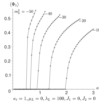
Figure 2: Phase transition with $\kappa_{s}$

We have a second order phase transition to a broken symmetry sector as we increase the $\kappa_{s}$ value, and so decrease the lattice temperature. This transition happens at lower and lower temperatures as one increases the lattice mass.

7.2 Evaluating the lattice temperature

To construct a true phase diagram we need to translate from the hopping parameter $\kappa_{s}$ to the lattice temperature $T$. Therefore we need to calculate the lattice temperature caused by particular choices of the $\kappa_{s}$ hopping parameter.

To do this we note that the presence of different hopping parameters in the temporal and spatial directions means that correlation functions will also be anisotropic with respect to the temporal and spatial axes of the lattice. The correlation length in lattice units in the time direction, $\xi_{t}$, will be different from the space-like correlation length, $\xi_{s}$. However, we expect the correlation lengths in physical units to be the same, even though the lattice spacings $a_{t}$ and $a_{s}$ will be different. This means that $a_{s}\xi_{s}\equiv a_{t}\xi_{t}$, which implies that

$$\frac{\xi_{t}}{\xi_{s}}=\frac{a_{s}}{a_{t}}=2Ta_{s}=\frac{2T}{\Lambda_{s}}$$ (24)

where $\Lambda_{s}$ is the spatial cutoff. By varying the spatial hopping parameter, $\kappa_{s}$, we will vary the relative size of the two correlation lengths and so vary the effective lattice anisotropy. This in turn allows us to vary the temperature [1].

The overall scale of the lattice temperature is set by $N_{t}=2$, which limits us to high temperatures, but within this range of high values we can vary the temperature continuously using the hopping parameter $\kappa_{s}$.

Now (5) gives

$$\frac{\partial F}{\partial\kappa_{s}}=-\frac{1}{N}\left\langle\sum_{n,i}\begin{picture}(10.0,1.0)\put(1.0,1.0){\circle*{0.5}} \put(1.0,1.0){\line(1,0){8.0}} \put(9.0,1.0){\circle*{0.5}} \end{picture}\right\rangle = -(d-1)\left\langle\Phi^{n_{4},\bf{n}*}\Phi^{n_{4},\bf{n}+\bf{e}_{i}}+\Phi^{n_{4},\bf{n}}\Phi^{n_{4},\bf{n}+\bf{e}_{i}*}\right\rangle=-(d-1)\xi_{s}$$

$$\frac{\partial F}{\partial\kappa_{t}}=-\frac{1}{N}\left\langle\sum_{n}\begin{picture}(4.0,8.0)\put(2.0,-3.0){\circle*{0.5}} \put(2.0,-3.0){\line(0,1){8.0}} \put(2.0,5.0){\circle*{0.5}} \end{picture}\right\rangle = -\left\langle(1+\mu_{L})\Phi^{n_{4},\bf{n}*}\Phi^{n_{4}+1,\bf{n}}+(1-\mu_{L})\Phi^{n_{4},\bf{n}}\Phi^{n_{4}+1,\bf{n}*}\right\rangle=-\xi_{t}$$ (25)

$$\Rightarrow \frac{T}{\Lambda_{s}}=\frac{(d-1)}{2}\frac{\partial F}{\partial\kappa_{t}}\left/\frac{\partial F}{\partial\kappa_{s}}\right.$$

Therefore purely by taking numerical derivatives with respect to the hopping parameters we can construct the lattice temperature for a given value of $\kappa_{s}$. As an example we plot $\ln(T/\Lambda_{s})$ against $\ln(\kappa_{s})$ for a particular range of physical parameters in Figure 3.

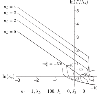
Figure 3: Effective T

In the unbroken regime of physical parameters there is a simple inverse relationship $\kappa_{s}T=k$. This is true for both zero and non-zero chemical potential. The only effect of the chemical potential is to change the value of the constant $k$. In the unbroken regime we find an almost perfect fit for the empirical curve

$$\kappa_{s}T=\frac{1}{2}\left(\mu_{L}^{2}+3\right)$$ (26)

However, as we pass through what is a second order phase transition, the relationship becomes more complex. This break-off point occurs at lower and lower $\kappa_{s}$ as one decreases the lattice mass.

For any other set of physical parameters we can similarly evaluate the effective temperature given by a particular choice of $\kappa_{s}$.

7.3 Phase transition using $T$

We can now combine the information in sections 7.1 and 7.2 to allow us to evaluate $\left\langle\Phi_{1}\right\rangle$ as a function of $T$ and look for a phase transition. This leads to the curves shown in Fig. 4.

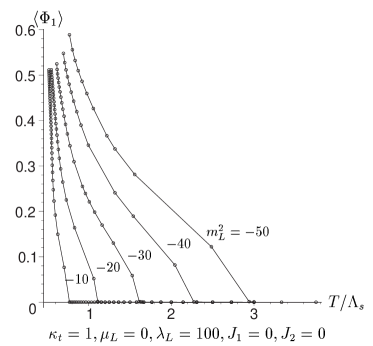
Figure 4: Phase transition with $T$

These curves follow directly from Fig. 2 and, as expected, as the temperature is lowered the symmetry breaks at some point, starting first with the lowest mass. The phase transition is second order in form. As the temperature decreases towards zero there is an unexpected divergence of the value of $\left\langle\Phi_{1}\right\rangle$. However, this is precisely in the regime where the approximation we are using is expected to break down, so no physical interpretation should be made of this behaviour.

7.4 Phase transition using $m_{L}^{2}$

For completeness we show the standard symmetry breaking which occurs as one lowers the physical mass. This second-order phase transition is discussed in much more detail in [4]. For particular choices of physical parameters we have the phase transition curves shown in Figure 5.

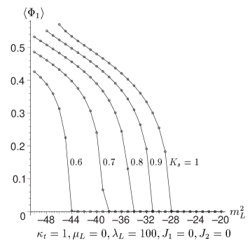
Figure 5: Phase transition with $m_{L}^{2}$

As expected, lowering the lattice mass breaks the symmetry, starting first with the highest $\kappa_{s}$ curve. The phase transition is second order. The curves are performed at fixed hopping parameter values and not at fixed lattice temperature. In the unbroken phase, as we can see in Fig. 3, the effective lattice temperature is independent of the lattice mass, so fixing $\kappa_{s}$ is equivalent to fixing $T$. However, when the symmetry is broken the temperature becomes mass dependent. Although this make things more complex it does not stop us from measuring the lattice temperature at the phase transition. Using the empirical formula (26) we can calculate the lattice temperatures. $\kappa_{s}=0.6,0.7,0.8,0.9$ and $1.0$ correspond to $T=2.499,2.143,1.875,1.667$ and $1.5$ respectively.

7.5 Phase transition using $\mu_{L}$

Having seen how the symmetry is restored as one increases the temperature and lattice mass, we should finally look at evaluating $\left\langle\Phi_{1}\right\rangle$ as a function of $\mu_{L}$. The phase transition with $\mu_{L}$ involves travelling between variational parameter spaces which look like Fig. 1(a) and Fig. 1(c). This means that we will have first-order phase transitions. Examining the free energy across the transition leads to the curves shown in Figure 6.

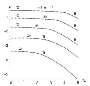
Figure 6: Phase transition in F with $\mu_{L}$

In the $m_{L}^{2}=-15\cdots-25$ plots we can see that there is a kink in the free energy due to the first order phase transition from an unbroken (U) to a broken (B) global $U(1)$ symmetry. The transition point moves to lower $\mu$ values as the mass is decreases. These curves have variational parameter spaces which move between Fig. 1(a) and Fig. 1(c). The kinks arise as one jumps from the unbroken to the broken minima in the variational parameter space.

At $m_{L}^{2}<-30$, and lower, the symmetry is broken for all $\mu$ values. The variational parameter space moves between Fig. 1(b) and Fig. 1(d). The symmetry is already broken at $\mu_{L}=0$ because of the second order phase transition which occurs at low enough temperatures, as discussed in section 7.4. The special case of the $m_{L}^{2}=-30$ curve is discussed in more detail later.

Using the free energy data, and again noting (23), we can construct the $\left\langle\Phi_{1}\right\rangle$ value. Where there is a kink in the $F$ value we expect a first order phase transition in the field value. This is precisely the behaviour seen for the curves in Figure 7.

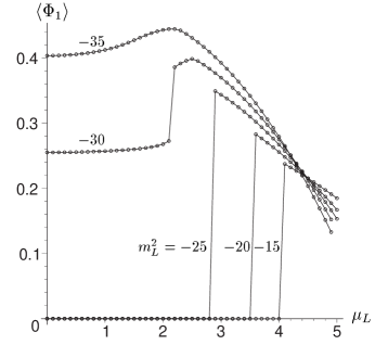
Figure 7: Phase transition in $\left\langle\Phi_{1}\right\rangle$ with $\mu_{L}$

In the $m_{L}^{2}=-15\cdots-25$ plots we see there is a first order phase transition from an unbroken to a broken global $U(1)$ symmetry. Crossing through this phase transition we move from Fig. 1(a) to Fig. 1(c) in variational space. Raising the chemical potential breaks the symmetry, starting first with the lowest $m_{L}^{2}$ curve. The transition point moves to higher $\mu_{L}$ values as one raises the lattice mass.

The $m_{L}^{2}=-30$ case is more unusual because, although the symmetry is already broken at $\mu_{L}=0$, we find evidence for a further phase transition at $\mu_{L}=2.1$. It turns out that this unexpected behaviour occurs at the place in phase space where the first order phase transition meets the second order phase transition. We shall postpone discussion of this point, as it will become much clearer on consideration of the full phase diagram, see section 7.6.

For $m_{L}^{2}<-30$ we see that the symmetry is already completely broken. There is a smooth crossover as one increases the chemical potential value from zero and in doing this one moves from Fig. 1(b) to Fig. 1(d) in variational parameter space.

Just as in section 7.4 these curves are derived at fixed hopping parameter values and not at fixed lattice temperature. However, unlike the lattice mass, the temperature is chemical potential dependent, whether or not one is in the broken regime. Each point on the curves is at a different lattice temperature. Again this make things more complex but we can still find the lattice temperature at the phase transition. We find that that $\{m_{L}^{2}=-15,\mu_{L}=4\}$ gives $T=9.5$, $\{m_{L}^{2}=-20,\mu_{L}=3.5\}$ gives $T=7.625$, $\{m_{L}^{2}=-25,\mu_{L}=2.9\}$ gives $T=5.705$, and finally $\{m_{L}^{2}=-30,\mu_{L}=2.1\}$ gives $T=3.705$.

7.6 Phase diagrams

7.6.1 $\{T,\mu_{L}\}$ Phase diagram

Combining all the information from the previous sections we can build up phase diagrams for the theory in $\{T,\mu_{L}\}$ space. These are plotted for various value of the lattice mass in Figure 8.

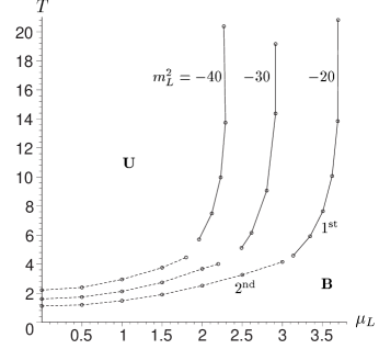
Figure 8: $\{T,\mu_{L}\}$ Phase diagram

Close to the $\mu_{L}=0$ axis we have a second-order phase transition between the unbroken phase at high temperatures and the broken phase at low temperatures. As one crosses through this transition the minima plots change from Fig. 1(a) to Fig. 1(c). However, as one follows this transition out to higher densities it becomes first order in nature. For the first order phase transition the minima plots change from Fig. 1(a) to Fig. 1(b).

For a small region at the changeover between the first-order and second-order phase transition lines both the minima at $~{}-\lambda_{L}$ and the minima at $~{}m_{L}^{2}$ are present in variational parameter space. Travelling from the second-order regime into the first-order part the minima at $~{}m_{L}^{2}$ spawn two further minima which rapidly move up towards $~{}-\lambda_{L}$. This is captured in the variational parameter space picture seen in Figure 9.

Figure 9: Changeover region

As $\mu_{L}$ and $T$ are increased further one enters the first-order phase transition regime and the two minima at $~{}m_{L}^{2}$ become one minimum.

It is this overlap which explains the unusual phase structure seen for the $m_{L}^{2}=-30$ curve in Fig. 7. We can that the unexpected additional first-order transition for this curve sits at $\mu_{L}=2.1,T=3.7$, which is right in the changeover regime for the $m_{L}^{2}=-30$ case in Fig. 8. For $\mu_{L}<2.1$ the field value is being evaluated at one of a pair of minima at $~{}m_{L}^{2}$, for the $\mu_{L}>2.1$ the field value is being evaluated at a pair of minima at $~{}-\lambda_{L}$. The jump between the two causes the first-order phase transition.

In physical space we have the three distinct types of pictures on the broken side of the transition, these are shown in Fig. 10.

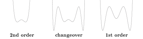
Figure 10: Qualitative $F$ against $\left\langle\Phi_{1}\right\rangle$ curves along the phase transition line

As one moves through the changeover area, starting from the second-order area of the phase diagram, the first-order style metastable states appear out beyond the second-order style minima. Then as one moves into the first-order area the two second-order minima merge to give the classic first-order field distribution.

7.6.2 $\{T,\rho\}$ Phase diagram

One can also calculate the charge density in lattice units which, noting that $\mathcal{H}_{eff}=\mathcal{H}+\mu\mathcal{Q}$ and $\mu_{L}=a_{t}\mu$, is

$$\rho:=\frac{\left\langle\mathcal{Q}\right\rangle}{N_{s}a_{s}^{3}}=2T\frac{\partial F}{\partial\mu_{L}}$$ (27)

where, because we are in lattice units, $a_{s}=\Lambda_{s}=1$. Using (27) one can construct the phase diagram of temperature against charge density. This is plotted in Figure 11.

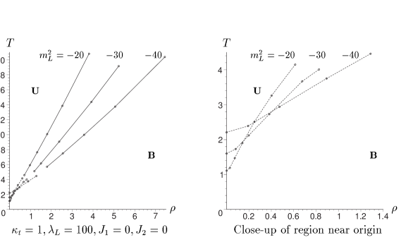
Figure 11: $\{T,\rho\}$ Phase diagram

The lower ends of the transition lines move closer to the origin in $\{T,\rho\}$ space as one increases the mass. In the close-up of the second-order phase transition lines, near to the $\mu=0$ axis, we can see an interesting complex curve form. As the transition becomes first-order for higher chemical potentials the transition lines become straighter.

8 Conclusions

An LDE optimisation of the standard hopping parameter expansion has allowed access to some of the truly non-perturbative physics of the scalar global $U(1)$ model. Close to the $\mu_{L}=0$ axis we find the expected second-order phase transition but as we track out to higher chemical potentials we see that this transition becomes first order. At our level of approximation at least there appears to be evidence for a more complex phase structure than expected.

Although the $U(1)$ model is in itself intrinsically interesting as a simple model for Higgs physics, the work in this paper can also be seen as a test of LDE techniques as applied to phase transition at finite density in general. In this context we can see that the LDE is a sucessful approach. The presence of the additional variational parameters allows one to examine a theory as one tracks through the phase transition with any of the physical parameters. By the choice of variational parameter one can actually choose which particular equivalent broken vacuum state the model is in, as demonstrated in [4]. Also the form of the free energy contours in variational parameter space signals the phase-space behaviour of the physical model itself. This allows one to extract the physical phase of the system without explicitly calculating the particular order parameter such as $\left\langle\Phi_{1}\right\rangle$.

To extend our approach to plotting out a phase diagram at finite density to a more complex model, in particular a gauge theory, we need to find an equivalent, lattice regularised, expansion to optimise. The hopping parameter expansion is only available for scalar theories: the derivative terms cannot be broken up in the same way for a gauge field theory. However, there is an alternative lattice expansion in the strong coupling expansion, i.e. an expansion in powers of the trace round lattice plaquettes. An example of an LDE optimisation of a plaquette expansion for gauge theories on the lattice at zero temperature and chemical potential is given in [8]. Using a similar scheme to that used in this paper for scalars one could extend considerations of gauge theories on the lattice to finite temperature and densities.

9 Acknowledgements

We are grateful to R.J. Rivers for useful discussions. D. Winder also gratefully acknowledges the financial support of the Particle Physics and Astronomy Research Council.

A Diagrams

Below we list all the diagrams which contribute to the cumulant expansion for the free energy of a $U(1)$ scalar Higgs model with finite temperature and chemical potential up and including order 3. With a lattice of two temporal links in extent we have periodicity across some of the diagrams. Points which are identified as identical are signified with an open circle in the diagrams. In the multiplicities that accompany the diagrams we have omitted the overall $N$ factor and used the shorthand

$$d_{j}=2(d-1)-j,$$ (28)

where $d$ is the spacetime dimension of the lattice and $j\in\mathcal{Z}$.

	$m_{1,1}=\frac{1}{2}d_{0}$		$m_{1,2}=1$
	$m_{2,1}=\frac{1}{2}d_{0}$		$m_{2,2}=d_{0}d_{1}$
	$m_{2,3}=2d_{0}$		$m_{2,4}=2d_{0}$
	$m_{2,5}=1$		$m_{2,6}=2$
	$m_{3,1}=\frac{1}{2}d_{0}$		$m_{3,2}=3d_{0}d_{1}$
	$m_{3,3}=3d_{0}d_{1}^{2}$		$m_{3,4}=d_{0}d_{1}d_{2}$
	$m_{3,5}=3d_{0}$		$m_{3,6}=3d_{0}$
	$m_{3,7}=6d_{0}d_{1}$		$m_{3,8}=3d_{0}d_{1}$
	$m_{3,9}=6d_{0}^{2}$		$m_{3,10}=3d_{0}d_{1}$
	$m_{3,11}=6d_{0}d_{1}$		$m_{3,12}=3d_{0}$
	$m_{3,13}=3d_{0}$		$m_{3,14}=3d_{0}$
	$m_{3,15}=6d_{0}$		$m_{3,16}=3d_{0}$
	$m_{3,17}=3d_{0}$		$m_{3,18}=1$
	$m_{3,19}=3$

References

- [1] I. Montvay and G. Münster Quantum Fields on a Lattice (Cambridge Monographs on Mathematical Physics, Cambridge, 1994).
- [2] J.I. Kapusta, Finite Temperature Field Theory (Cambridge University Press, Cambridge, 1989)
- [3] J.M. Yeomans, Statistical Mechanics of Phase Transitions (Oxford Science Publications, Oxford, 1992)
- [4] T.S. Evans, M. Ivin and M. Möbius, An optimized pertubation expansion for a global O(2) theory, Nucl. Phys.B577 (2000) 325.
- [5] H.F. Jones, Nucl. Phys. (Proc.Suppl.) B39 (1995) 220.
- [6] H.F. Jones and P. Parkin, The Renormalised Thermal Mass with Non-zero charge density, [hep-th/0005069].
- [7] H.F. Jones, P. Parkin and D. Winder, Quantum Dynamics of the Slow Rollover Transition in the Linear Delta Expansion, [hep-th/0008069].
- [8] J.O. Akeyo and H.F. Jones, Phys. Rev. D 47 (1993) 1668.
- [9] J.O. Akeyo and H.F. Jones, Z. Phys. C 58 (1993) 629.
- [10] J.O. Akeyo, H.F. Jones and C.S. Parker, Extended Variational Approach to the SU(2) Mass Gap on the Lattice, Phys. Rev. D 51 (1995) 1298 [hep-ph/9405311].
- [11] T.S. Evans, H.F. Jones and A. Ritz, An Analytical Approach to Lattice Gauge-Higgs Models, in “Strong and Electroweak Matter ’97”, ed. F.Csikor and Z.Fodor (World Scientific, Singapore, 1998, ISBN 981-02-3257-8) [hep-ph/9707539].
- [12] T.S. Evans, H.F. Jones and A. Ritz, On the Phase Structure of the 3D SU(2)-Higgs Model and the Electroweak Phase Transition, Nucl. Phys. B517 (1998) 599 [hep-ph/9710271].
- [13] A. Duncan and H.F. Jones, Phys. Rev. D 47 (1993) 2560.
- [14] I.R.C. Buckley, A. Duncan and H.F. Jones, Phys. Rev. D 47 (1993) 2554.
- [15] C.M. Bender, A. Duncan and H.F. Jones, Phys. Rev. D 49 (1994) 4219.
- [16] C.M. Bender, K.A. Milton, S.S. Pinsky and L.M. Simmons Jr., J. Math. Phys. 30 (1989) 1447.
- [17] W. Kerler and T. Metz, Phys. Rev. D 44 (1991) 1263.
- [18] X.-T. Zheng, Z.G. Tan and J. Wang, Nucl. Phys. B287 (1987) 171.
- [19] X.-T. Zheng, B.S. Liu, Intl. J. Mod. Phys. A 6 (1991) 103.
- [20] Jens O. Andersen, Eric Braaten and Michael Strickland, The massive thermal basketball diagram[ hep-ph/0002048 ].
- [21] A.N. Sissakian, I.L. Solovtsov and O.P. Solovtsova, Phys. Lett. B 321 (1994) 381.
- [22] V.I. Yukalov, J. Math. Phys. 33 (1992) 3994.
- [23] C.M. Wu et al., Phase Structure of Lattice Theory by Variational Cumulant Expansion, Phys. Lett. B 216 (1989) 381.
- [24] W.E. Caswell, Ann. Phys. 123 (1979) 153.
- [25] J. Killingbeck, J. Phys. A 14 (1981) 1005.
- [26] A. Okapińska, Phys. Rev. D 35 (1987) 1835.
- [27] A. Okapińska, Phys. Rev. D 36 (1987) 2415.
- [28] J.M. Yang, J. Phys. G 17 (1991) L143.
- [29] J.M. Yang, C.M. Wu and P.Y. Zhao, J. Phys. G 18 (1992) L1.
- [30] P.M. Stevenson, Phys. Rev. D 23 (1981) 2916.
- [31] D.E. Groom et al, Particle Physics Databook, Eur. Phys. J. C15 1 (2000)
- [32] T.S. Evans, in “Fourth Workshop on Thermal Field Theories and their Applications”, 5-10 August 1995, Dalian, China, ed. Y.X. Gui, F.C. Khanna, and Z.B. Su (World Scientific, Singapore, 1996) p.283-295 (hep-ph/9510298).
- [33] M. Lüscher and P. Weisz, Application of the Linked Cluster expansion to the n-component theory (Nuclear Physics B 300, 325-359, 1988)
- [34] M. Lüscher and P. Weisz, Nucl. Phys. B300 (1989) 325.
- [35] M. Wortis, Linked Cluster Expansion, in “Phase Transitions and Critical Phenomena”, vol.3, eds. C. Domb and M.S. Green (Academic Press, London, 1974).
- [36] T. Reisz, Hopping Parameter Series construction for Models with Nontrivial Vacuum (hep-lat/9802023, 17 Feb 1998)
- [37] T. Reisz, Advanced Linked Cluster Expansion. Scalar fields at finite temperature (hep-lat/9505023, 29 May 1995)
- [38] H. Meyer-Ortmanns and T. Reisz, Nucl. Phys. (Proc.Suppl.) B73 (1999) 892