The GDH Sum Rule and Related Integrals

Abstract

The spin structure of the nucleon resonance region is analyzed on the basis of our phenomenological model MAID. Predictions are given for the Gerasimov-Drell-Hearn sum rule as well as generalized integrals over spin structure functions. The dependence of these integrals on momentum transfer is studied and rigorous relationships between various definitions of generalized Gerasimov-Drell-Hearn integrals and spin polarizabilities are derived. These results are compared to the predictions of chiral perturbation theory and phenomenological models.

I introduction

Since the end of the 1970’s, the spin structure of the nucleon has been studied by scattering polarized lepton beams off polarized targets. The aim of such experiments has been to measure the spin structure functions $g_{1}(x,Q^{2})$ and $g_{2}(x,Q^{2})$, depending on the fractional momentum of the constituents, $x=Q^{2}/2m\nu$, and the square of four-momentum transfer, $q^{2}=-Q^{2}$, where $\nu$ is the (virtual) photon lab energy and $m$ the nucleon mass. Already the first experiments at CERN [1] and SLAC [2] sparked considerable interest in the community, because the first moment of $g_{1}$ , $\Gamma_{1}(Q^{2})=\int\limits_{0}^{1}g_{1}(x,Q^{2})dx$, turned out to be substantially below the quark model prediction [3]. This ”spin crisis” led to the conclusion that less than half of the nucleon spin is carried by the quarks. However, the difference of the proton and neutron moments, $\Gamma_{1}^{p}-\Gamma_{1}^{n}$ , was found to be well described by Bjorken’s sum rule [4], which is a strict QCD prediction.

In spite of new and more sophisticated experiments [5], the question about the carriers of the spin is still open. Various new experimental proposals are presently underway at HERMES, COMPASS and Jlab [6], and in the context of the ELFE project [7]. The idea behind these experiments is to measure the so-called skewed parton distributions, which are expected to reveal information on details of the parton structure, such as sea quark, gluon and orbital momentum contributions to the spin. The experimental tool to determine these new structure functions will be semi-inclusive reactions such as deeply virtual Compton scattering and the production of various mesons as filters of particular quantum numbers [7].

Recent improvements in polarized beam and target techniques have made it possible to determine the spin structure functions over an increased range of kinematical values. In particular the E143 Collaboration at SLAC [8] and the HERMES Collaboration at DESY [9] have obtained data at momentum transfers down to $Q^{2}\simeq 1$ (GeV/c)². The range of momentum transfer below these values will be covered by various experiments at the Jefferson Lab, which are being performed in the full range $0.02(GeV/c)^{2}\leq Q^{2}\leq 2$ (GeV/c)² [10]. The first direct experimental data for real photons $(Q^{2}=0)$ were recently taken at MAMI [11] in the energy range 200 MeV$<\nu<800$ MeV, and data at the higher energies are expected from ELSA within short.

In conclusion we expect that the spin structure functions will soon be known over the full kinematical range. This will make it possible to study the transition from the non-perturbative region at low $Q^{2}$ to the perturbative region at large $Q^{2}$. In particular the first moment $\Gamma_{1}$ is constrained, in the limit of $Q^{2}\rightarrow 0$ (real photons), by the famous Gerasimov-Drell-Hearn sum rule (GDH, Ref. [12]), $\Gamma_{1}\rightarrow-Q^{2}\kappa^{2}_{N}/8m^{2}$ , where $\kappa_{N}$ is the anomalous magnetic moment of the nucleon. The reader should note that here and in the following we have included the inelastic contributions to $\Gamma_{1}$ only. As has been pointed out by Ji and Melnitchouk [13], the elastic contribution is in fact the dominant one at small $Q^{2}$ and has to be taken into account in comparing with twist expansions about the deep inelastic limit.

The GDH sum rule predicts $\Gamma_{1}<0$ for small $Q^{2}$, while all experiments for $Q^{2}>1$ (GeV/c)² yield clearly positive values for the proton. Therefore, the spin structure has to change rapidly at low $Q^{2}$, with some zero-crossing at $Q^{2}<1$ (GeV/c)². The expected strong variation of $\Gamma_{1}$ with momentum transfer marks the transition from the physics of resonance-driven coherent processes to incoherent scattering off the constituents. The evolution of the sum rule was first described by Anselmino et al. [14] in terms of a parametrization based on vector meson dominance. Burkert, Ioffe and others [15, 16, 17] refined this model considerably by treating the contributions of the resonances explicitly. Soffer and Teryaev [18] suggested that the rapid fluctuation of $\Gamma_{1}$ should be analyzed in conjunction with $\Gamma_{2}$ , the first moment of the second spin structure function. The latter is constrained by the less familiar Burkhardt-Cottingham sum rule (BC, Ref. [19]) at all values of $Q^{2}$. Therefore the sum of the two moments, $\Gamma_{3}=\Gamma_{1}+\Gamma_{2}$, is known for both $Q^{2}=0$ and $Q^{2}\rightarrow\infty$. Though this sum is related to the practically unknown longitudinal-transverse interference cross section $\sigma^{\prime}_{LT}$ and therefore not yet determined directly, Ref. [18] assumed that it can be extrapolated smoothly between the two limiting values of $Q^{2}$. The rapid fluctuation of $\Gamma_{1}$ then follows by subtraction of the BC value from $\Gamma_{3}$.

The small momentum evolution of a generalized GDH integral was investigated by Bernard et al. [25] in the framework of heavy baryon ChPT. At $O(p^{3})$ these authors predicted a positive slope of this integral at $Q^{2}=0$, while the phenomenological analysis of Burkert et al. [15] indicated a negative slope. These generalized GDH integrals contain information on both spin structure functions, which are combined such that the practically unknown longitudinal-transverse interference term cancels. As will be explained later in detail, the definition of these integrals in the literature is not unique.

Recently, Ji et al. [21] have extended the calculations to $O(p^{4})$. They find strong modifications due to the next-order term, which even change the sign of the slope at the origin to negative values much below the phenomenological analysis. In a similar way the related forward spin polarizability $\gamma_{0}$ is changed substantially by going from $O(p^{3})$ to $O(p^{4})$ , which may cast some doubt on the convergence of the perturbation series [22, 23, 24, 26]. Unfortunately there appears an additional problem concerning the decomposition of the Compton amplitude in the nucleon pole terms (contained in the real Born amplitude) and contributions of intermediate excited states (the complex residual amplitude). The origin of the problem is due to the Foldy-Wouthuysen type expansion in HBChPT, which changes the pole structure at any given expansion in the nucleon mass $m$.

It will be the aim of this contribution to present our predictions for the helicity-dependent cross sections, and to compare our results with the existing data and other theoretical predictions. For this purpose we shall review the formalism in sect. 2, with special emphasis on sum rules and generalized GDH integrals. Our predictions will be compared to the data and previous calculations in sect. 3, and we shall close by a brief summary of our results in sect. 4.

II Formalism

We consider the scattering of polarized electrons off polarized target nucleons. The $lab$ energies of the electrons in the initial and final states are denoted with $E$ and $E^{\prime}$, respectively. The incoming electrons carry the (longitudinal) polarization $h=\pm 1$, and the two relevant polarization components of the target are $P_{z}$ (parallel to the $lab$ momentum $\vec{k}$ of the virtual photon) and $P_{x}$ (perpendicular to $\vec{k}$ in the scattering plane of the electron and in the half-plane of the outgoing electron). The differential cross section for exclusive electroproduction can then be expressed in terms of four “virtual photoabsorption cross sections” $\sigma_{i}(\nu,Q^{2})$ by [27, 28]

$$\frac{d\sigma}{d\Omega\ dE^{\prime}}=\Gamma\sigma(\nu,Q^{2})\,,$$ (1)

$$\sigma=\sigma_{T}+\epsilon\sigma_{L}+hP_{x}\sqrt{2\epsilon(1-\epsilon)}\ \sigma^{\prime}_{LT}+hP_{z}\sqrt{1-\epsilon^{2}}\sigma^{\prime}_{TT}\,,$$ (2)

with

$$\Gamma=\frac{\alpha}{2\pi^{2}}\ \frac{E^{\prime}}{E}\ \frac{K}{Q^{2}}\ \frac{1}{1-\epsilon}$$ (3)

the flux of the virtual photon field and $\epsilon$ its transverse polarization, $\nu=E-E^{\prime}$ the virtual photon energy in the $lab$ frame and $Q^{2}>0$ describing the square of the virtual photon four-momentum. In accordance with our previous notation [29] we shall define the flux with the “photon equivalent energy” $K=K_{H}=(W^{2}-m^{2})/2m=\nu(1-x)$, where $W$ is the total $cm$ energy, $m$ the mass of the target nucleon, and $x=Q^{2}/2m\nu$ the Bjorken scaling variable. We note that our choice of the flux factor is originally due to Hand [30]. Another often used definition was given by Gilman [31] who used $K=K_{G}=\nu\sqrt{1+\gamma^{2}}$, the $lab$ momentum of the virtual photon, with $\gamma=Q/\nu$.

The quantities $\sigma_{T}$ and $\sigma^{\prime}_{TT}$ can be expressed in terms of the total cross sections $\sigma_{3/2}$ and $\sigma_{1/2}$, corresponding to excitation of intermediate states with spin projections $3/2$ and $1/2$, respectively,

$$\sigma_{T}=\frac{1}{2}(\sigma_{3/2}+\sigma_{1/2})\,,\qquad\sigma^{\prime}_{TT}=\frac{1}{2}(\sigma_{3/2}-\sigma_{1/2})\ .$$ (4)

The virtual photoabsorption cross sections in Eq. (2) are related to the quark structure functions $F_{1}$, $F_{2}$, $g_{1}$, and $g_{2}$ depending on $\nu$ and $Q^{2}$,

$$\sigma_{T} = \frac{4\pi^{2}\alpha}{mK}\ F_{1}\ ,$$ (5)

$$\sigma_{L} = \frac{4\pi^{2}\alpha}{K}\left[\frac{F_{2}}{\nu}(1+\gamma^{2})-\frac{F_{1}}{m}\right]\ ,$$ (6)

$$\sigma^{\prime}_{LT} = -\frac{4\pi^{2}\alpha}{mK}\,\gamma\,(g_{1}+g_{2})\ ,$$ (7)

$$\sigma^{\prime}_{TT} = -\frac{4\pi^{2}\alpha}{mK}\left(g_{1}-\gamma^{2}\,g_{2}\right)\ .$$ (8)

In comparing with the standard nomenclature of deep inelastic scattering DIS [8] we note that $\sigma^{\prime}_{LT}=-\sigma_{LT}(DIS)$ and $\sigma^{\prime}_{TT}=-\sigma_{TT}(DIS)$. It is obvious that the virtual absorption cross sections $\sigma_{i}$ depend on the choice of the flux factor $K$. In the following we shall use the definition of Hand, $K=K_{H}$. If we compare with the work of authors using the convention of Gilman, $K=K_{G}$, our photoabsorption cross sections of Eqs. (5) have to be multiplied by the ratio $K_{H}/K_{G}=(1-x)/\sqrt{1+\gamma^{2}}$, i.e. $\sigma_{i}^{G}=(1-x)(1+\gamma^{2})^{-1/2}\sigma_{i}^{H}$.

We generalize the Gerasimov-Drell-Hearn (GDH) sum rule [12] by introducing the $Q^{2}$-dependent integral

$$I_{1}(Q^{2})=\frac{2m^{2}}{Q^{2}}\int_{0}^{x_{0}}g_{1}(x,Q^{2})\ dx\rightarrow\left\{\begin{array}[]{lll}-\frac{1}{4}\kappa_{N}^{2}&{\rm for}&Q^{2}\rightarrow 0\\ \frac{2m^{2}}{Q^{2}}\Gamma_{1}+{\cal O}(Q^{-4})&{\rm for}&Q^{2}\rightarrow\infty\end{array}\right.\,,$$ (9)

where $x_{0}=Q^{2}/(2mm_{\pi}+m_{\pi}^{2}+Q^{2})$ is the threshold for one-pion production. In the scaling regime the structure functions should depend on $x$ only, and $\Gamma_{1}=\int g_{1}(x)dx=const$.

For the second spin structure function the Burkhardt-Cottingham (BC) sum rule asserts that the integral over $g_{2}$ vanishes if integrated over both elastic and inelastic contributions [19]. As a consequence one finds

$$I_{2}(Q^{2})=\frac{2m^{2}}{Q^{2}}\int_{0}^{x_{0}}g_{2}(x,Q^{2})\ dx=\frac{1}{4}\frac{G_{M}(Q^{2})-G_{E}(Q^{2})}{1+Q^{2}/4m^{2}}\,G_{M}(Q^{2})\,,$$ (10)

i.e. the inelastic contribution for $0<x<x_{0}$ equals the negative value of the elastic contribution given by the $rhs$ of Eq. (10), which is parametrized by the magnetic and electric Sachs form factors $G_{M}$ and $G_{E}$, respectively. In the limit of $Q^{2}\rightarrow 0$, these form factors are normalized to the magnetic moment $\mu_{N}=\kappa_{N}+e_{N}$ and the charge $e_{N}$ of the nucleon, $G_{M}(0)=\mu_{N}$ and $G_{E}(0)=e_{N}$. The BC sum rule has the limiting cases

$$I_{2}(Q^{2})\rightarrow\left\{\begin{array}[]{lll}\frac{1}{4}\mu_{N}\kappa_{N}&{\rm for}&Q^{2}\rightarrow 0\\ {\cal O}(Q^{-10})&{\rm for}&Q^{2}\rightarrow\infty\end{array}\right.\,.$$ (11)

By use of Eqs. (5) the integrals $I_{1}$ and $I_{2}$ can be cast into the form

$$I_{1}(Q^{2})=\frac{m^{2}}{8\pi^{2}\alpha}\int_{\nu_{0}}^{\infty}\frac{1-x}{1+\gamma^{2}}\left(\sigma_{1/2}-\sigma_{3/2}-2\gamma\,\sigma^{\prime}_{LT}\right)\ \frac{d\nu}{\nu}\ ,$$ (12)

$$I_{2}(Q^{2})=\frac{m^{2}}{8\pi^{2}\alpha}\int_{\nu_{0}}^{\infty}\frac{1-x}{1+\gamma^{2}}\left(\sigma_{3/2}-\sigma_{1/2}-\frac{2}{\gamma}\,\sigma^{\prime}_{LT}\right)\ \frac{d\nu}{\nu}\ ,$$ (13)

where $\nu_{0}=m_{\pi}+(m_{\pi}^{2}+Q^{2})/2m$ is the threshold $lab$ energy of one-pion production.

Since $\gamma\sigma^{\prime}_{LT}={\cal O}(Q^{2})$, the longitudinal-transverse term does not contribute to the integral $I_{1}$ in the real photon limit. However, the ratio $\sigma^{\prime}_{LT}/\gamma$ remains constant in that limit and hence contributes to $I_{2}$. As a result we find

$$I_{2}(0)=\frac{1}{4}\kappa_{N}^{2}+\frac{1}{4}e_{N}\kappa_{N}\ ,$$ (14)

with the two terms on the $rhs$ corresponding to the contributions of $\sigma_{3/2}-\sigma_{1/2}$ and $\sigma^{\prime}_{LT}$, respectively.

It follows from Eqs. (12) and (13) that the sum of the integrals $I_{1}$ and $I_{2}$ is solely determined by the longitudinal-transverse interference term,

$$I_{3}(Q^{2}) = I_{1}(Q^{2})+I_{2}(Q^{2})=\frac{2m^{2}}{Q^{2}}\int_{0}^{x_{0}}(g_{1}+g_{2})dx$$ (15)

$$= -\frac{m^{2}}{4\pi^{2}\alpha}\int_{\nu_{0}}^{\infty}(1-x)\left(\frac{\nu}{Q}\sigma^{\prime}_{LT}\right)\frac{d\nu}{\nu}\ ,$$ (16)

with $I_{3}(0)=\frac{1}{4}e_{N}\ \kappa_{N}$. In Eq. (15) and in the following equations we have suppressed the arguments of the spin structure functions and virtual photoabsorption cross sections, $(x,Q^{2})$ and $(\nu,Q^{2})$ respectively. Of course, the integrals of Eq. (15) will only converge if $\sigma^{\prime}_{LT}$ drops faster than $1/\nu$ for large values of $\nu$. The origin of this problem is, of course, already contained in Eq. (13), and there are severe doubts whether the $I_{2}$ integral is actually converging.

As we have seen above, $I_{1}(Q^{2})$ approaches the GDH integral in the limit $Q^{2}\rightarrow 0$. However, at finite $Q^{2}$ the longitudinal-transverse term contributes significantly. In order to eliminate this term, 3 choices have been made in the literature [32], which in the following will be labeled $N=A,B$, and $C$,

$$I_{A}\,(Q^{2}) = \frac{m^{2}}{8\pi^{2}\alpha}\int_{\nu_{0}}^{\infty}(1-x)\ (\sigma_{1/2}-\sigma_{3/2})\frac{d\nu}{\nu}$$ (17)

$$= \frac{2m^{2}}{Q^{2}}\int_{0}^{x_{0}}(g_{1}-\gamma^{2}\ g_{2})\ dx\ ,$$ (18)

$$I_{B}\,(Q^{2}) = \frac{m^{2}}{8\pi^{2}\alpha}\int_{\nu_{0}}^{\infty}\frac{1-x}{\sqrt{1+\gamma^{2}}}\ (\sigma_{1/2}-\sigma_{3/2})\frac{d\nu}{\nu}$$ (19)

$$= \frac{2m^{2}}{Q^{2}}\int_{0}^{x_{0}}\frac{1}{\sqrt{1+\gamma^{2}}}\ (g_{1}-\gamma^{2}\ g_{2})\ dx\ ,$$ (20)

$$I_{C}\,(Q^{2}) = \frac{m^{2}}{8\pi^{2}\alpha}\int_{\nu_{0}}^{\infty}(\sigma_{1/2}-\sigma_{3/2})\frac{d\nu}{\nu}$$ (21)

$$= \frac{2m^{2}}{Q^{2}}\int_{0}^{x_{0}}\frac{1}{1-x}\,(g_{1}-\gamma^{2}\ g_{2})\ dx\ .$$ (22)

It is obvious that definition A is the natural choice in terms of the quark structure functions. On the other hand, the definitions B and C look “natural” in terms of the transverse-transverse cross section $\sigma^{\prime}_{TT}$ if one chooses the definition of the virtual photon flux according to Gilman or Hand, respectively. As we shall show in the following section, the numerical differences between these 3 definitions are quite substantial, in particular with regard to (I) the slopes at $Q^{2}=0$ and (II) the positions of the zero crossing.

Concerning the slopes of the generalized GDH integrals at $Q^{2}=0$, we find the following model-independent relations

$$I_{B}^{\prime}-I_{A}^{\prime} = -\frac{m^{2}}{4\alpha}\frac{1}{4\pi^{2}}\int\frac{d\nu}{\nu^{3}}(\sigma_{1/2}-\sigma_{3/2})\ ,$$ (23)

$$I_{C}^{\prime}-I_{A}^{\prime} = -\frac{m}{4\alpha}\frac{1}{4\pi^{2}}\int\frac{d\nu}{\nu^{2}}(\sigma_{1/2}-\sigma_{3/2})\ ,$$ (24)

$$I_{1}^{\prime}-I_{A}^{\prime} = -\frac{m^{2}}{2\alpha}\frac{1}{4\pi^{2}}\int\frac{d\nu}{\nu^{3}}(\sigma_{1/2}-\sigma_{3/2})-\frac{m^{2}}{2\alpha}\frac{1}{2\pi^{2}}\int\frac{d\nu}{\nu^{3}}\lim_{Q^{2}\to 0}\left(\frac{\nu}{Q}\sigma^{\prime}_{LT}\right)\ ,$$ (25)

where $I^{\prime}=dI/dQ^{2}$ and all cross sections should be evaluated at $Q^{2}=0$. In particular we observe the appearance of the forward spin polarizability,

$$\gamma_{0}=\frac{1}{4\pi^{2}}\int\frac{d\nu}{\nu^{3}}(\sigma_{1/2}-\sigma_{3/2})\ ,$$ (26)

and the longitudinal-transverse polarizability

$$\delta_{0}=-\frac{1}{2\pi^{2}}\int\frac{d\nu}{\nu^{3}}\lim_{Q^{2}\to 0}\left(\frac{\nu}{Q}\sigma^{\prime}_{LT}\right)\ ,$$ (27)

which can be evaluated pretty safely on the basis of dispersion relations.

Finally we give the multipole decomposition of the cross sections for the dominant one-pion contribution,

$$\sigma^{\prime}_{TT}(1\pi) = 4\pi\frac{k^{cm}_{\pi}}{K^{cm}}\sum_{l}\frac{1}{2}(l+1)[-(l+2)(|E_{l+}|^{2}+|M_{l+1,-}|^{2})$$ (29)

$$+l(|M_{l+}|^{2}+|E_{l+1,-}|^{2})-2l(l+2)(E_{l+}^{\ast}M_{l+}-E^{\ast}_{l+1,-}M_{l+1,-})]$$

$$= 4\pi\frac{k^{cm}_{\pi}}{K^{cm}}\{-|E_{0+}|^{2}+|M_{1+}|^{2}-6E_{1+}^{\ast}M_{1+}-3|E_{1+}|^{2}+|E_{2-}|^{2}\pm\ ...\}\,$$ (30)

$$\sigma^{\prime}_{LT}(1\pi) = 4\pi\frac{k^{cm}_{\pi}}{K^{cm}}\left(\frac{Q}{\omega^{cm}_{\gamma}}\right)\sum_{l}\frac{1}{2}(l+1)^{2}$$ (32)

$$\cdot\ [-L_{l+}^{\ast}((l+2)E_{l+}+lM_{l+})+L_{l+1,-}^{\ast}(lE_{l+1,-}+(l+2)M_{l+1,-})]$$

$$= 4\pi\frac{k^{cm}_{\pi}}{K^{cm}}\left(\frac{Q}{\omega^{cm}_{\gamma}}\right)\{-L_{0+}^{\ast}E_{0+}-2L_{1+}^{\ast}(M_{1+}+3E_{1+})$$ (34)

$$+L_{1-}^{\ast}M_{1-}+2L_{2-}^{\ast}E_{2-}\pm\ ...\}\ .$$

We note that here and in the following, expressions as $E_{l+}^{\ast}M_{l+}$ should be read as Re$(E_{l+}^{\ast}M_{l+})$. The kinematical variables in Eqs. (29) and (32) are $K^{cm}=\frac{W^{2}-m^{2}}{2W},\ \omega^{cm}_{\gamma}=\frac{m\nu-Q^{2}}{W}$ and $k^{cm}_{\pi}=\frac{1}{2W}\sqrt{(W^{2}-m_{\pi}^{2})^{2}-2m^{2}(W^{2}+m_{\pi}^{2})+m^{4}}$, where $W=\sqrt{m^{2}+2m\nu-Q^{2}}$ is the total $c.m.$ energy. Since $L_{0+}$ has a zero at $\omega^{cm}_{\gamma}=0$, it is often convenient to use the Coulomb or “scalar” multipoles defined by

$$S_{l\pm}=\frac{k^{cm}_{\gamma}}{\omega^{cm}_{\gamma}}\ L_{l\pm}\ ,\$$ (35)

with $k^{cm}_{\gamma}=\frac{m}{W}\sqrt{\nu^{2}+Q^{2}}\$ .

In particular Eq. (25) can be cast into the form

$$I_{1}^{\prime}-I_{A}^{\prime}=-\frac{m^{2}}{2\alpha}(\gamma_{0}-\delta_{0})\ ,$$ (36)

with the forward spin polarizability

$$\gamma_{0}=\frac{2}{\pi}\int\frac{d\nu}{\nu^{3}}\frac{k_{\pi}^{cm}}{\nu}\sqrt{1+\frac{2\nu}{m}}\{\mid E_{0+}\mid^{2}-\mid M_{1+}\mid^{2}+6E_{1+}^{\ast}M_{1+}+3\mid E_{1+}\mid^{2}\pm\ ...\}$$ (37)

and the longitudinal-transverse polarizability

$$\delta_{0}=\frac{2}{\pi}\int\frac{d\nu}{\nu^{3}}\frac{k_{\pi}^{cm}}{\nu}\left(1+\frac{2\nu}{m}\right)\{L_{0+}^{\ast}E_{0+}+2L_{1+}^{\ast}(M_{1+}+3E_{1+})\pm\ ...\}\ .$$ (38)

Due to the weight factor $\nu^{-3}$ in the integral for $\gamma_{0}$, Eq. (37), the contribution of s-wave pion production $(E_{0+})$ is enhanced such that it nearly cancels the contribution of magnetic $\Delta$ excitation $(M_{1+})$. Though the electric quadrupole excitation is small, $E_{1+}/M_{1+}\approx-2.5\%$ for real photons, its interference term with the magnetic dipole excitation becomes quite important for the forward spin polarizability because of the mentioned cancellation. However, such a cancellation does not occur in the case of $\delta_{0}$, Eq. (38). The Fermi-Watson theorem asserts that $L_{l\pm},\ E_{l\pm}$ and $M_{l\pm}$ have the same phases in the region of interest below two-pion threshold, and gauge invariance requires that $E_{l\pm}=L_{l\pm}$ in the Siegert limit or “pseudo threshold” situated in the unphysical region. The latter relation changes in the physical region, and as a rule of thumb we find $L_{0+}\approx\frac{1}{2}E_{0+}$ and $L_{1+}\approx 2E_{1+}$ in the (physical) threshold region. Since the p-wave contribution in Eq. (38) is much suppressed, there is no substantial cancellation between s and p waves, and as a result the longitudinal-transverse term gives the dominant contribution to the difference of slopes between $I_{1}$ and $I_{A}$, e.g. in Eq. (36).

III Results and Discussion

The spin structure of the nucleon is described by the cross sections $\sigma_{3/2}\,-\,\sigma_{1/2}$ and $\sigma^{\prime}_{LT}$, which are plotted in Figs. 1 and 2 as functions of the total energy $W$ for $Q^{2}=0,0.5$ and $1.0\,(GeV/c)^{2}$. In the upper part of Fig. 1, at $Q^{2}=0$, the negative contribution near threshold is essentially due to s-wave production of charged pions. Due to the weighting with $\nu^{-1}$ and $\nu^{-3}$, for the GDH integral and the spin polarizability respectively, s-wave pions become increasingly important in comparison with p-wave production near the $\Delta(1232)$, which carries the opposite sign. At the photon point, $Q^{2}=0$, the second and third resonance regions are clearly visible, their contributions have the same sign as for the $\Delta$.

With increasing momentum transfer $Q^{2}$, the cross sections generally decrease as is to be expected. However, there are two interesting peculiarities, which are of some consequence for the $Q^{2}$ dependence of the generalized GDH integrals.

1. The negative bump due to s-wave pion production near threshold decreases rapidly with increasing values of $Q^{2}$ due to the form factor. In the case of the $\Delta$, this effect is mostly compensated by the increase of the p-wave multipole appearing with the 3-momentum of the virtual photon. As a result the $\Delta$ effects become rapidly more dominant at very small $Q^{2}$.

2. The contributions in the second and third resonance region, which added to the $\Delta$ contribution at $Q^{2}=0$, change sign at $Q^{2}\approx 0.5\,(GeV/c)^{2}$.

The general decrease due to form factors and the change of sign in the first vs. second and third resonance regions lead to a rapid decrease of the integrals in absolute values.

The second structure function $\sigma_{LT}^{{}^{\prime}}$ is shown in Fig. 2. This longitudinal-transverse cross section vanishes, of course, for real photons. However, it contributes to the Burkhardt-Cottingham sum rule even in the limit $Q^{2}\,\to\,0$ due to Eq. (13), where it appears multiplied by a factor $\nu/Q$ in the integral. In Fig. 2 we therefore show both $2\gamma\sigma^{{}^{\prime}}_{LT}$ and $2\sigma^{{}^{\prime}}_{LT}/\gamma$, which contribute to the $I_{1}$ and $I_{2}$ integrals, respectively. Obviously the convergence of $2\sigma^{{}^{\prime}}_{LT}/\gamma$ is bad, even after the weighting with $\nu^{-1}$ in Eq. (13). The different sign of s-wave and $\Delta$ contributions is also seen in Fig. 2. Since $L_{1+}/M_{1+}$ is of the order of $5\%$ for real photons, the $\Delta$ resonance appears in that case as a small bump on a large negative background. Again the s-wave threshold contribution decreases rapidly with increasing $Q^{2}$, such that the $\Delta$ resonance becomes the dominant feature for $Q^{2}=1$ (GeV/c)² and $W<1.3$ GeV. Due to the increasingly negative contribution for larger energies, however, the integral over the longitudinal-transverse cross sections of Fig. 2 will always take the negative sign, such that the contribution of $\sigma^{\prime}_{LT}$ to $I_{1}$ and $I_{2}$ (see Eqs. (12) and (13)) will be positive at every value of $Q^{2}$.

The dependence of various generalized GDH integrals on momentum transfer is shown in Figs. 3-5. We include the one-pion channel according to MAID [29] and the two-pion and eta channels as in our previous work [28]. It is obvious that the integrals $I_{A},\ I_{B}$, and $I_{C}$ with purely transverse cross sections in the integrand (see Fig. 4) behave fundamentally different from $I_{1}$ (see Fig. 3), which also gets contributions from the longitudinal-transverse interference. While the latter has a large positive slope at the origin and crosses the zero line around $Q^{2}=0.4\,(GeV/c)^{2}$, the former 3 integrals have negative slopes at the origin, which leads to zero-crossings at much larger $Q^{2}$. The minima of the generalized GDH integrals occur at very small momentum transfers, indeed, as may be seen in more detail in Fig. 5. Such negative slopes at the origin were first obtained by Burkert, Ioffe and others [15, 16] in the framework of phenomenological models. In a similar spirit Scholten and Korchin [17] have recently evaluated $I_{A}(Q^{2})$ in the framework of an effective Lagrangian model. Their results are in qualitative agreement with those of Fig. 5, in particular they also predict a minimum at $Q^{2}=0.5\,(GeV/c)^{2}$. However, it is worthwhile pointing out that the different definitions lead to quite different results amongst each other. It is therefore absolutely prerogative to give clear definitions before comparing the published experimental or theoretical values. Concerning such definitions we find it most convenient to express the integrals in terms of the spin structure functions $g_{1}$  and $g_{2}$, because these are uniquely defined in the literature.

As mentioned in section 1, there have been many phenomenological estimates for the GDH sum rule of the nucleon. Until recently the estimates for the GDH integral of the proton were in the range from -260 $\mu$b to -290 $\mu$b, while the sum rule predicted -204 $\mu$b [33]. Our present analysis is shown in Table I. In the region 200 MeV$<\nu<$800 MeV we can now rely on the experimental data taken in 1998 at MAMI [11]. We are quite confident about our estimate for the integrand between threshold and 200 MeV, because here the cross sections are largely determined by s-wave pion production via the amplitude $E_{0+}$ fixed through low energy theorems. Also our estimate for one-pion production in the energy range 800 MeV$<\nu<$ 1.6 GeV should be quite reliable, because our model MAID describes the helicity structure of the main resonances very well. Since $\eta$ production has now been measured over a large energy range, and because of its $S_{11}$ dominance, the helicity structure of that contribution is fixed. The situation is less clear with regard to $K^{+}$ production, but the overall contribution of this reaction should be small. The only major uncertainty is with regard to two-pion production at the higher energies, which has been estimated with the prescription of Ref. [34].

As can be seen from Table I, the contributions of one-pion production from below $200~{}$MeV and above $800~{}$MeV cancel almost. The still missing DIS contribution has been estimated by Bianchi et al. [20] from an extrapolation of DIS to real photons. If we add those $(26\pm 7)~{}\mu$b to our analysis in the resonance region, the total result for the proton is $(-202\pm 10)~{}\mu$b. While the agreement between analysis and sum rule is remarkably good for the proton, this does not yet end the story. In fact our present prediction for the neutron is off the sum rule value by about $60~{}\mu$b, i.e. $25\%$!

The slope of the integral $I_{C}$ was first obtained by Bernard et al. [25] in chiral perturbation theory (ChPT) to $O(p^{3})$, with the result

$$I_{C}^{\prime}=\frac{1}{6}m^{2}\left(\frac{g_{A}}{4\pi m_{\pi}f_{\pi}}\right)^{2}\ .$$ (39)

Recently, Ji et al. [21] have calculated the slope of the integral $I_{A}$ up to terms of $O(p^{4})$, with the result

$$I_{A}^{\prime}=\frac{1}{6}m^{2}\left(\frac{g_{A}}{4\pi m_{\pi}f_{\pi}}\right)^{2}\Bigg{\{}1-\frac{\pi}{4}\frac{m_{\pi}}{m}(13+2\tau_{3}+2\kappa_{V})\Bigg{\}}\ .$$ (40)

By comparing Eqs. (39) and (40) we conclude that $I_{A}^{\prime}$ and $I_{C}^{\prime}$ take the same value at $O(p^{3})$. The reason for this becomes obvious from the model-independent relations Eqs. (23) - (25). While the $rhs$ of Eqs. (23) and (25) is $O(m^{2}/m_{\pi}^{2})$, as follows explicitly from the ChPT result for the forward spin polarizability $\gamma_{0}$, the $rhs$ of Eq. (24) is $O(m/m_{\pi})$, i.e. one order higher in the chiral counting scheme. Clearly the $(m/m_{\pi})^{2}$ or $(m/m_{\pi})$ behavior of the $rhs$ is due to the fact that the integrals diverge like $m_{\pi}^{-2}$ or $m_{\pi}^{-1}$, respectively, if the lower limit of the integrals, $\nu_{0}\simeq m_{\pi}$, goes to zero.

The slope of $I_{1}$, on the other hand, vanishes to $O(p^{3})$. To next order the result is [21]

$$I_{1}^{\prime}=\frac{1}{6}m^{2}\left(\frac{g_{A}}{4{\pi}m_{\pi}f_{\pi}}\right)^{2}\frac{\pi}{8}\,\frac{m_{\pi}}{m}\,(1+3\kappa_{V}+2\tau_{3}+6\kappa_{S}\tau_{3})\ .$$ (41)

The forward spin polarizability was first calculated to $O(p^{3})$ by Bernard et al. [22]. Again large corrections were found in the next order, $O(p^{4})$, by Ji et al. [23] and Kumar et al. [24]. However, Gellas et al. [26] claim that these authors used a definition of $\gamma_{0}$ that differed from the usual definition through forward dispersion relations as in Eq. (37), i.e. that the spin polarizabilities of Refs. [23, 24] contain higher order contributions from the nucleon pole term. The origin of the problem is due to the fact that HBChPT relies on nonrelativistic expansions of the intermediate state propagators, which makes it difficult to separate the pole terms from the internal structure contributions that are related to the polarizabilities. The two results for $\gamma_{0}$ at $O(p^{4})$ read [26, 23, 24]

$$\gamma_{0}\ {\rm{(GHM)}}=\frac{2}{3}\alpha\left(\frac{g_{A}}{4\pi\,m_{\pi}f_{\pi}}\right)^{2}\,\Bigg{\{}1-\frac{\pi}{8}\frac{m_{\pi}}{m}\,(13+4\tau_{3}+\kappa_{V}-\kappa_{S}\tau_{3})\Bigg{\}}\ ,$$ (42)

$$\gamma_{0}\ {\rm{(JKO,\ KMB)}}=\frac{2}{3}\alpha\left(\frac{g_{A}}{4\pi\,m_{\pi}f_{\pi}}\right)^{2}\,\Bigg{\{}1-\frac{\pi}{8}\frac{m_{\pi}}{m}\,(15+6\tau_{3}+3\kappa_{V}+\kappa_{S}\tau_{3})\Bigg{\}}\ .$$ (43)

The value of $\delta_{0}$ can then be obtained by the model-independent relation Eq. (36). If we assume that the results for $I_{A}^{\prime}$ and $I_{1}^{\prime}$ of Ref. [21] are valid, Eqs. (40)-(43) lead to the expressions

$$\delta_{0}\ {\rm{(GHM)}}=\frac{1}{3}\alpha\left(\frac{g_{A}}{4\pi\,m_{\pi}f_{\pi}}\right)^{2}\,\Bigg{\{}1+\frac{\pi}{8}\frac{m_{\pi}}{m}\,(1-2\tau_{3}+5\kappa_{V}+8\kappa_{S}\tau_{3})\Bigg{\}}\ ,$$ (44)

$$\delta_{0}\ {\rm{(JKO,\ KMB)}}=\frac{1}{3}\alpha\left(\frac{g_{A}}{4\pi\,m_{\pi}f_{\pi}}\right)^{2}\,\Bigg{\{}1-\frac{\pi}{8}\frac{m_{\pi}}{m}\,(3+6\tau_{3}-\kappa_{V}-4\kappa_{S}\tau_{3})\Bigg{\}}\ .$$ (45)

The values for the polarizabilities of the proton are compared to our results in table II. Here and in the following all numerical expressions are obtained with $\kappa_{V}=3.71$ and $\kappa_{S}=-0.12$ the isovector and isoscalar combinations of the anomalous magnetic moments, $g_{A}=1.26$ the axial coupling constant, $f_{\pi}=$92.4 MeV the pion decay constant, $m=$ 938 MeV the proton mass, and $m_{\pi}=$138 MeV an average pion mass.

The upper part of table II shows a partial wave decomposition of the polarizabilities. As has been pointed out before, the contributions of s and p waves nearly cancel in the case of $\gamma_{0}$, while $\delta_{0}$ is largely dominated by s waves. In the central part of table II, we give the contributions of various energy bins. Due to the weighting factor $\nu^{-3}$, the threshold region below 200 MeV contributes substantially, while the region above 800 MeV is of little importance. In the case of $\gamma_{0}$, the integrand in the resonance region (200 MeV$<\nu<$800 MeV) has now been measured at MAMI [11]. The experimental value is (-1.71$\pm$0.09) $10^{-4}$ fm⁴, slightly smaller than the prediction of MAID, -1.66$\cdot 10^{-4}$ fm⁴. We conclude that the presently best value of the forward spin polarizability is $\gamma_{0}=(-0.70\pm 0.10)\,10^{-4}~{}$fm⁴. Comparing now with the results of ChPT at $O(p^{3})$, we find the interesting relation $\gamma_{0}=2\delta_{0}$, which can be explained as follows. The leading order term originates from the lower limit of the integrals in Eqs. (25) and (26) if $\nu_{0}\simeq m_{\pi}\rightarrow 0$. In that limit the threshold amplitudes [35] for charged pion production are $E_{0^{+}}^{\rm{thr}}(\pi^{+})=2L_{0^{+}}^{\rm{thr}}(\pi^{+})$. By comparing Eqs. (37) and (38) in the same limit, $\nu$ and $m_{\pi}\ll m$, all higher partial waves vanish and we are left with integrands $\nu^{-2}$ times $\mid E_{0^{+}}\mid^{2}$ and $L_{0^{+}}^{\ast}E_{0^{+}}$, respectively, which immediately leads to the mentioned relation. Given the existing ambiguity in the definition of $\gamma_{0}$ in HBChPT , it is probably not very useful to compare the phenomenological results with the predictions of ChPT. A brief look at the last 4 lines of table II shows, however, that neither prediction can presently describe both $\gamma_{0}$ and $\delta_{0}$. It would therefore be interesting to examine whether the higher order terms in $I_{1}^{\prime}$ etc. could possibly also be affected by the ambiguities to separate elastic and inelastic contributions.

In table III we compare our predictions for the slopes of the integrals of Eqs. (12)-(21) with the predictions of ChPT, the Burkhardt-Cottingham sum rule, and the models of Anselmino et al., and Soffer and Teryaev. We should point out that we have evaluated all predictions with the same set of coupling constants and masses as specified before. Furthermore, we have used the more recent value $\Gamma_{1}^{p}=0.146$ for the asymptotic value [36] of the integral over the spin structure function $g_{1}$, and the proton radii $\langle r^{2}\rangle_{M}^{p}=0.728$ fm² and $\langle r^{2}\rangle_{E}^{p}=0.717$ fm² as given in Ref. [37].

It is obvious that the different approaches lead to rather different results. In particular, the generalized GDH integrals differ by factors and, with regard to ChPT at $O(p^{3})$, even by sign. In the case of $I_{B}$ we can estimate the asymptotic contribution, which is missing in our analysis, from the HERMES data [9]. If we add the slope of this contribution to our value, we obtain a further decrease by about $20\%$, i.e. a final result of $I_{B}^{\prime}\approx-4$ (GeV/c)^-2, which is still different from ChPT by a factor of 3. As has been pointed out before, the $O(p^{3})$ calculation predicts $I_{A}^{\prime}=I_{C}^{\prime}$ and $I_{1}^{\prime}=0$. If we use our model-independent Eqs. (23) and (36) and the relation $\gamma_{0}=2\delta_{0}$ at $O(p^{3})$, we find $I_{B}^{\prime}=0$. In a similar way we have evaluated $I_{B}^{\prime}=-6.6$ GeV^-2 at $O(p^{4})$ from the results of Ji et al. [21, 23]. Had we taken the value of $\gamma_{0}$ from Ref. [26], the result would be $I_{B}^{\prime}=-12.6$ GeV^-2. As a consequence the ambiguity in the $O(p^{4})$ spin polarizabilities influences the predictions for the generalized GDH integrals and a solution of the problem is urgently called for. We recall that this problem arises from the difficulty to describe the proper pole structure for real and virtual Compton scattering in higher order HBChPT, and repeat our suspicion that similar ambiguities could also arise in the case of the GDH integrals.

We further note that our analysis does not support the conjecture of Soffer and Teryaev [18] that $I_{3}=I_{1}+I_{2}$ varies slowly with $Q^{2}$. These authors propose to parametrize $I_{3}$ for the proton by a smooth function interpolating between the given values for $Q^{2}=0$ and $Q^{2}\rightarrow\infty$,

$$I_{3}\,(Q^{2})=\left\{\begin{array}[]{r@{\quad,\quad}l}\kappa_{p}/4-2m^{2}\,Q^{2}\,\Gamma^{p}_{1}/Q_{0}^{4}&Q^{2}<Q_{0}^{2}\\ 2m^{2}\,\Gamma^{p}_{1}/Q^{2}&Q^{2}>Q_{0}^{2}\ .\end{array}\right.$$ (46)

The continuity of the function and its derivative is implemented by choosing $Q_{0}^{2}=16m^{2}\,\Gamma^{p}_{1}/\kappa_{p}\simeq 1$ (GeV/c)². The resulting derivative at the origin is very small,

$$I_{3}^{\prime}=-\frac{\kappa^{2}_{p}}{128m^{2}\,\Gamma^{p}_{1}}\approx-0.2~{}{\rm{GeV}}^{-2}\ ,$$ (47)

and the derivative of $I_{1}$ follows from assuming the validity of the BC sum rule. In comparing our result with Eq. (47), we find that the slopes differ by about a factor of 20.

The model of Anselmino et al. [14], on the other hand, is relatively close to our prediction. Motivated by the vector dominance model, these authors proposed to describe $I_{1}$ by the expression

$$I_{1}\,(Q^{2})=\frac{1}{(Q^{2}+m_{V}^{2})^{2}}\left(2m\Gamma^{p}_{1}\,Q^{2}\,-\frac{\kappa^{2}_{p}}{4}\,m_{V}^{4}\right)\ ,$$ (48)

with $m_{V}\approx m_{\rho}$, the mass of the $\rho$ meson. The resulting derivative at the origin is

$$I_{1}^{\prime}=\frac{\kappa^{2}_{p}}{2m_{V}^{2}}+\frac{2m^{2}\Gamma^{p}_{1}}{m_{V}^{4}}\simeq 3.4~{}{\rm{GeV}}^{-2}\,$$ (49)

while our phenomenological model predicts 4.4 GeV^-2.

IV SUMMARY

The results of our phenomenological model MAID have been presented for various spin observables. We have updated our prediction for the GDH sum rule for the proton and find a good agreement with the sum rule value. The change from earlier results originate from a collaborative effect of a correct treatment of the threshold region, a reduced estimate for the two-pion contributions based on the recent results of the GDH Collaboration at MAMI, and an asymptotic contribution. We look forward to the continuation of the MAMI experiments to the higher energy at ELSA, which will probe the weakest point of our prediction, the two-pion contribution in the resonance region. In the case of the neutron the disagreement remains, and we are urgently waiting for a direct measurement of the helicity-dependent neutron cross sections in the resonance region.

The same model can be used to calculate the spin polarizability and an associated longitudinal-transverse polarizability. Due to the weighting factor $\nu^{-3}$, these predictions are on rather firm ground. Unfortunately, a comparison with the results from ChPT is difficult, because their interpretation is still under discussion.

We have also presented a systematic analysis of various generalized GDH-type integrals $I_{\rm{GDH}}(Q^{2})$ and of the BC sum rule $I_{2}(Q^{2})$. In the case of the proton, the latter can be reasonably well described by our model, but our prediction for the neutron fails again. Though all generalized GDH integrals are fixed for both real photons, $Q^{2}=0$, and in the asymptotic region, $Q^{2}\rightarrow\infty$, their dependence on momentum transfer differs considerably for $Q^{2}\lesssim 1$ (GeV/c)². A clear signature of these differences are the slopes $I_{\rm{GDH}}^{\prime}=dI_{\rm{GDH}}/dQ^{2}$ at the origin. In particular we compare our predictions to those of other phenomenological models and heavy baryon chiral perturbation theory. The different slopes from different definitions of $I_{\rm{GDH}}$ are related by model-independent relations involving the spin polarizability and related quantities, which can be safely evaluated from the helicity-dependent cross sections in the resonance region. Since both the spin polarizability and the derivatives of the GDH integrals are derived from doubly virtual Compton scattering in chiral perturbation theory, the ongoing discussion on how to separate pole and non-pole contributions in that theory also poses a serious problem for the generalized GDH integrals. As long as this problem exists, the given comparison between different predictions should not be taken too seriously. However the large spread of the obtained values certainly poses the challenge to solve the theoretical problem and to measure the generalized GDH integrals a soon as possible. Since we expect a negative slope of the purely transverse GDH integrals with a minimum as low as $Q^{2}\simeq m_{\pi}^{2}$, it is quite fortunate that some of the JLab experiments take data down to very low momentum transfer.

We conclude that the presently running and newly proposed experiments with beam and target/recoil polarization will give invaluable information on the spin structure of the nucleon. It is to be hoped that this quantitative increase of our knowledge will also sharpen our theoretical tools to test the applicability and the predictions of QCD in the confinement region.

ACKNOWLEDGEMENT

The authors gratefully acknowledge the support of the Deutsche Forschungsgemeinschaft (SFB 443) and of the Heisenberg-Landau program. We would like to thank the members of the GDH Collaboration for many fruitful discussions, in particular H.-J. Arends, R. Lannoy, and A. Thomas.

TABLE I.: Contributions to the GDH sum rule for the proton in units of $\mu$b. Note that $\nu=1.66\,GeV$ corresponds to $W=2\,GeV.$

energy range	channels	contributions	reference
$\nu_{0}<\nu<200$ MeV	$\pi^{+}n$	31	MAID [29]
	$\pi^{0}p$	-1
200 MeV$<\nu<800$ MeV	all	-218$\pm$6	MAMI [11]
800 MeV$<\nu<1.66$ GeV	$\pi^{+}n$	-30	MAID [29]
	$\pi^{0}p$	-6
	$\eta$ p	7	our estimate
	$\pi\pi$ N	-15$\pm$ 8
	$\Lambda K^{+},\Sigma K^{+}$	4
$\nu>1.66$ GeV	all	26 $\pm$7	Bianchi et al. [20]
total	all	-202 $\pm$ 10
sum rule	all	-204	GDH [12]

TABLE II.: Contributions to $\gamma_{0}$ and $\delta_{0}$ for the proton in units of $10^{-4}$fm⁴. The quantities with an asterisk are evaluated by use of Eqs. (44) and (45). For details see text.

contributions		$\gamma_{0}$	$\delta_{0}$	reference
one-pion	l=0	$2.65$	$2.03$	MAID [29]
	l=1	$-2.90$	$-0.36$
	l$\geq$ 2	$-0.39$	$-0.01$
others	$n\pi+\eta$	$-0.01$	$0.00$	our estimate
total		$-0.65$	$1.66$
$\nu_{0}<\nu<200$ MeV		$1.04$	$0.81$	MAID [29]
200 MeV $<\nu<800$ MeV		$-1.66$	$0.82$
800 MeV $<\nu<1.6$ GeV		$-0.03$	$0.02$	our estimate
total		$-0.65$	$1.66$
ChPT $O(p^{3})$		$4.6$	$2.3^{\ast}$	BKM [22]
ChPT $O(p^{4})$		$-3.9$	$1.5^{\ast}$	JKO [21], KMB [24]
		$-0.9$	$4.5^{\ast}$	GHM [26]

TABLE III.: Slopes of GDH related integrals for the proton at $Q^{2}=0$ in units of GeV^-2. The quantities with an asterisk are evaluated by use of Eq. (23) and with $\gamma_{0}$ as given by the respective authors. For details see text.

$I_{1}^{\prime}$	$I_{2}^{\prime}$	$I_{3}^{\prime}$	$I_{A}^{\prime}$	$I_{B}^{\prime}$	$I_{C}^{\prime}$	reference
$4.4$	$-8.8$	$-4.4$	$-4.8$	$-3.4$	$-5.6$	MAID [29]
	$-8.2$					BC [19]
$0$			$9.1$	$0^{\ast}$	$9.1$	$O(p^{3})$ BKM [25]
$7.0$			$-14.4$	$-6.6^{\ast}$		$O(p^{4})$ JKO [23]
$3.4$						AIL [14]
$8.0$	$-8.2$	$-0.2$				ST [18]

FIG. 1.: Helicity difference $\sigma_{3/2}-\sigma_{1/2}$ for the proton at $Q^{2}=0,\,\,0.5$ and 1.0 (GeV/c)² Dashed, dotted and dash-dotted curves: contributions of single-pion, eta and multipion channels, respectively; solid curves: total result.

FIG. 2.: Longitudinal-transverse cross sections for the proton, $2\gamma\sigma^{{}^{\prime}}_{LT}$ (solid curves) and $2\sigma^{{}^{\prime}}_{LT}/\gamma$ (dashed curves) at $Q^{2}=0,\,\,0.5$ and 1.0 (GeV/c)². The calculations are for the one-pion channel only.

FIG. 3.: The integrals $I_{1}$, $I_{2}$ and $I_{3}$ for the protons and neutrons as functions of $Q^{2}$ and integrated up to $W_{max}=2$ GeV. Dashed curves are the results obtained without the $\sigma^{\prime}_{LT}$ contribution, solid curves are the total results, and dotted curves for the $I_{2}$ integrals are the prediction of the BC sum rule. The full circles at $Q^{2}=0$ are the GDH sum rule values. The open circles at $Q^{2}=0.5$ (GeV/c)² are the recent SLAC data [8] for the resonance region.

   

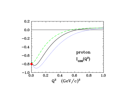
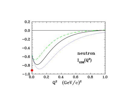
FIG. 4.: The GDH integrals $I_{A}$ (solid curves), $I_{B}$ (dashed curves) and $I_{C}$ (dotted curves) for proton and neutron, integrated up to $W_{max}=2$ GeV, in the range $0\leq Q^{2}\leq 1$ (GeV/c)². The full circles at $Q^{2}=0$ are the GDH sum rule values.

   

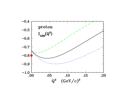
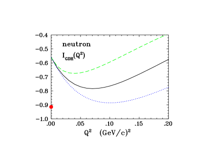
FIG. 5.: The GDH integrals $I_{A},\ I_{B},\$ and $I_{C},$ at small $Q^{2}$. Notation as in Fig. 4.

REFERENCES

- [1] J. Ashman et al. (EMC Collaboration), Nucl. Phys. B 238, 1 (1989).
- [2] G. Baum et al. (E130 Collaboration), Phys. Rev. Lett. 51, 1135 (1983).
- [3] J. Ellis and R. Jaffe, Phys. Rev. D 9, 1444 (1974) and D 10, 1669 (1974).
- [4] J. D. Bjorken, Phys. Rev. 148, 1467 (1966).
- [5] D. Adams et al. (SMC Collaboration), Phys. Lett. B 396, 338 (1997) and Phys. Rev. D 56, 5330 (1997).
- [6] See the review article by B. Lampe and E. Reya, Phys. Rep. 332, 1 (2000), and references quoted therein.
- [7] See the review article by M. Vanderhaeghen, hep-ph/0007232, and references quoted therein.
- [8] K. Abe et al. (E143 Collaboration), Phys. Rev. D 58, 112003 (1998).
- [9] K. Ackerstaff et al. (HERMES Collaboration), Phys. Lett. 44, 531 (1998).
- [10] V. D. Burkert et al., JLab proposal 91-23 (1991); S. Kuhn et al., JLab proposal 93-09 (1993); Z. E. Meziani et al., JLab proposal 94-10 (1994); J. P. Chen et al., JLab proposal 97-110 (1997).
- [11] J. Ahrens et al. (GDH Collaboration), Phys. Rev. Lett. 84, 5950 (2000), and private communications with members of the GDH Collaboration.
- [12] S.B. Gerasimov, Yad. Fiz. 2, 598 (1965), [Sov. J. Nucl. Phys. 2, 430 (1966)]; S. D. Drell and A. C. Hearn, Phys. Rev. Lett. 16, 908 (1966).
- [13] X. Ji and W. Melnitchouk, Phys. Rev. D 56, R1 (1997).
- [14] M. Anselmino, B. L. Ioffe, and E. Leader, Yad. Phys. 49, 214 (1989), [Sov. J. Nucl. Phys. 49, 136 (1989)].
- [15] V. D. Burkert and B. L. Ioffe, Phys. Lett. B 296, 223 (1992); V. D. Burkert and Zh. Li, Phys. Rev. D 47, 46 (1993); B. L. Ioffe, Yad. Fiz. 60, 1797 (1997) [Phys. At. Nucl. 60, 1558 (1997).
- [16] I. Aznauryan, Yad. Fiz. 58, 1088 (1995) [Phys. At. Nucl. 58, 1014 (1995)].
- [17] O. Scholten and A.Yu. Korchin, Eur. Phys. J. A6, 211 (1999).
- [18] J. Soffer and O. Teryaev, Phys. Rev. Lett. 70, 3373 (1993); Phys. Rev. D 51, 25 (1995); Phys. Rev. D 56, 7458 (1997).
- [19] H. Burkhardt and W. N. Cottingham, Ann. Phys. (N.Y.) 56, 453 (1970).
- [20] N. Bianchi and E. Thomas, Phys. Lett. B 450, 439 (1999).
- [21] X. Ji and J. Osborne, hep-ph/9905410; X. Ji, C.-W. Kao, and J. Osborne, Phys. Lett. B 472, 1 (2000).
- [22] V. Bernard, N. Kaiser, and U.-G. Meißner, Int. J. Mod. Phys. E 4, 193 (1995).
- [23] X. Ji, C.-W. Kao, and J. Osborne, Phys. Rev. D 61, 074003 (2000).
- [24] K. B. V. Kumar, J. A. McGovern, and M. Birse, hep-ph/9909442.
- [25] V. Bernard, N. Kaiser, and U.-G. Meißner, Phys. Rev. D 48, 3062 (1993).
- [26] G. C. Gellas, T. R. Hemmert, and U.-G. Meißner, Phys. Rev. Lett. 85, 14 (2000).
- [27] D. Drechsel, Prog. Part. Nucl. Phys. 34, 181 (1995).
- [28] D. Drechsel, S. S. Kamalov, G. Krein, and L. Tiator, Phys. Rev. D 59, 094021 (1999).
- [29] D. Drechsel, O. Hanstein, S.S. Kamalov and L. Tiator, Nucl. Phys. A 645, 145 (1999); MAID, an interactive program for pion electroproduction, available at www.kph.uni-mainz.de/MAID/.
- [30] L. N. Hand, Phys. Rev. 129, 1834 (1993).
- [31] F. J. Gilman, Phys. Rev. 167, 1365 (1968).
- [32] R. Pantförder, Ph.D thesis, Bonn, 1997; hep-ph/9805434.
- [33] D. Drechsel and G. Krein, Phys. Rev. D 58, 116009 (1998).
- [34] H. Holvoet and M. Vanderhaeghen, private communication.
- [35] S. Scherer and J. H. Koch, Nucl. Phys. A 534, 461 (1991).
- [36] M. Glück et al., Phys. Rev. D 53, 4775 (1996).
- [37] P. Mergell, U.-G. Meißner, and D. Drechsel, Nucl. Phys. A 596, 367 (1996).