Higher twist corrections and maxima for DIS
on a proton in the high density QCD region

Abstract

We show that the ratio of different structure functions have a maximum which depends on energy. We argue, using the Golec-Biernat and Wusthoff model as well as the eikonal approach, that these maxima are functions of the saturation scale. We analyze leading and higher twist contributions for different observables to check whether a kinematic region exists where high parton density effects can be detected experimentally.

1 Introduction

In this letter we continue our study of phenomena associated with gluon saturation in deep inelastic scattering (DIS) following our original study in Ref. [1]. Our goal is to find the kinematic region where the evolution of parton densities can no longer be correctly described by linear evolution equations[2, 3, 4, 5]. To solve this problem analytically one has to find a solution of the non-linear evolution equation which was derived in Refs. [6, 7] and in Ref. [8] in different approaches. In spite of the fact that the asymptotic solutions are known[9], a detailed description of the boundary of the saturation region is still lacking. We would like to determine how gluon saturation can be detected in current and future experimental data.

The idea suggested in Ref. [1] was that there is a breakdown of the Operator Product Expansion as one gets sufficiently close to the saturation region. This enabled us to find the scale $\hat{Q}^{2}$ where the twist expansion breaks down. Since, at sufficiently large $Q^{2}$, the saturation scale is the only scale of the problem, it should be expressed unambiguously in terms of $\hat{Q}^{2}$. We refer the reader to our previous publication for more details.

In Ref. [1] we used the eikonal model[10, 11, 12, 13, 14] to calculate the various structure functions relevant in DIS on nuclei, and then to expand them into the twist series. In this letter we will address the subject of DIS on a nucleon and apply the same approach developed for DIS on nuclei.

The paper is organized as follows: We start with a brief review of our approach without going into details of the calculation (Sec. 2). In Sec. 3, we discuss numerical estimates regarding the nucleon target. Finally, in Sec. 4 we conclude by proposing possible ways to measure the different twists at HERA and LHC.

2 The Model

As was pointed out in the introduction we use the eikonal (or Mueller-Glauber) model to calculate shadowing corrections. A complete description of the eikonal approach to shadowing corrections (SC) was given in Ref. [14]. It was shown in Ref. [14, 15, 16] that the eikonal approximation leads to a reasonable theoretical as well as experimental approximation in the region of not too small $x_{B}$. There are weighty arguments in favor of using the eikonal model to calculate contributions of different twists[1] in various cross sections. This simple eikonal model is a reasonable starting point for understanding how the shadowing corrections occur. The use of the Glauber-Mueller approach was justified for a nuclear target[6], and it should hold for a nucleon as well[17].

Following Ref. [1] and assuming that all dipoles in the virtual photon wave function have the size $r_{t}^{2}=4/Q^{2}$ and neglecting the quark masses we obtain for the longitudinal and transverse photon cross sections

$$\sigma_{L}(\gamma^{*}p) = 2\alpha_{em}\pi R^{2}\frac{Q_{s}^{2}}{4Q^{2}}G^{3\,2}_{3\,4}\left(\frac{Q^{2}}{Q_{s}^{2}}\Bigg{|}{0,1;\frac{5}{2}\atop 1,1,2;-\frac{1}{2}}\right)$$ (1)

$$\sigma_{T}(\gamma^{*}p) = 4\alpha_{em}\pi R_{A}^{2}\frac{Q_{s}^{2}}{4Q^{2}}\left[G^{3\,2}_{3\,4}\left(\frac{Q^{2}}{Q_{s}^{2}}\Bigg{|}{1,1;\frac{5}{2}\atop 1,1,1;\frac{1}{2}}\right)-\frac{1}{2}G^{3\,2}_{3\,4}\left(\frac{Q^{2}}{Q_{s}^{2}}\Bigg{|}{0,1;\frac{5}{2}\atop 1,1,1;-\frac{1}{2}}\right)\right.$$ (2)

$$\left.+\frac{Q_{s}^{2}}{Q^{2}}\left\{\frac{1}{4}G^{3\,2}_{3\,4}\left(\frac{Q^{2}}{Q_{s}^{2}}\Bigg{|}{1,1;\frac{7}{2}\atop 2,2,2;\frac{1}{2}}\right)-\frac{1}{2}G^{3\,2}_{3\,4}\left(\frac{Q^{2}}{Q_{s}^{2}}\Bigg{|}{1,2;\frac{7}{2}\atop 2,2,2;\frac{3}{2}}\right)\right\}\right]$$

where ${{}_{3}}F_{1}$ is the generalized hypergeometric function, $G^{3\,2}_{3\,4}$ is the Meijer function (see Ref.[18]), and we have defined

$$Q_{s}^{2}(x_{B},Q^{2})\equiv\frac{2\pi\alpha_{S}\,x_{B}G(x_{B},Q^{2})}{3R^{2}}\quad,$$ (3)

where $G(x_{B},Q^{2})$ denotes the gluon distribution in the nucleon, $R$ the radius of the nucleon, and $Q_{s}^{2}$ is used as a shorthand for $Q_{s}^{2}(x_{B},Q^{2})$ defined in Eq. (3). $Q_{s}^{2}$ is a saturation scale in the framework of our model.

Diffractive cross sections can be calculated using the simple relations following from the unitarity constraint:

$$\sigma(\gamma^{*}p)^{D}_{T,L}(Q_{s}^{2}/Q^{2})=\sigma(\gamma^{*}p)_{T,L}(Q_{s}^{2}/Q^{2})-\frac{1}{2}\sigma(\gamma^{*}p)_{T,L}(2Q_{s}^{2}/Q^{2})$$ (4)

Formulae Eq. (1), Eq. (2) and Eq. (4) make it possible to estimate the contribution of any order twist to the particular cross section[1] by closing the contour of integration in a Meijer function over the corresponding pole.

We argued in the Ref. [1], that studying ratios of the cross sections can yield very useful information about the saturation region. While the cross sections receive large corrections from the next-to-leading order of perturbative expansion, their ratios do not[14, 16]. In this paper we will consider two ratios $\sigma_{L}/\sigma_{T}$ and $\sigma_{L}^{D}/\sigma_{T}^{D}$. Both of these ratios display a remarkable property as a function of photon virtuality $Q^{2}$. At small $Q^{2}$ the ratios vanish since the real photon is transverse. At large $Q^{2}$ they vanish as well, as implied by pQCD. This leads us to suggest that both ratios have maximum $Q_{max}^{2}$. We would expect that this maximum is a certain function of the saturation scale, since at small $x_{B}$ and large $Q^{2}$ this is the only scale important in the process of dipole scattering. So, studying the behaviour of the $Q_{max}^{2}$ with energy we can determine the $Q_{s}^{2}(x_{B})$ as well. Two problems occur. First, the confinement scale affects the position of the maximum of ratios. We can only hope that at large energies (small $x_{B}$) the maximum will occur at sufficiently large $Q^{2}$ where this influence is small, though as we will see below, it cannot be completely excluded.

Second, we do not know the precise form of the function $Q_{s}^{2}=f(Q_{max}^{2})$ which has to be determined using the full twist expansion. We can, however, roughly estimate the form of this function using a simple approach. Namely, we illustrate the most important features (for finding the $Q_{max}^{2}$) of Eq. (1) and Eq. (2) by the following formulae which have the correct asymptotic behaviour for $Q^{2}\ll m_{f}^{2}<Q_{s}^{2}$ and $Q^{2}\gg Q_{s}^{2}>m_{f}^{2}$, and which are valid for any model:

$$\sigma_{T} \sim R^{2}\frac{Q_{s}^{2}}{Q^{2}+Q_{s}^{2}}\quad,$$

$$\sigma_{L} \sim R^{2}\frac{Q^{2}}{Q^{2}+m^{2}_{f}}\cdot\frac{Q_{s}^{2}}{Q^{2}+Q_{s}^{2}}\quad,$$

$$\sigma_{T}^{D} \sim R^{2}\frac{Q_{s}^{2}}{Q^{2}+Q_{s}^{2}}\quad,$$

$$\sigma_{L}^{D} \sim R^{2}\frac{Q^{2}}{Q^{2}+m^{2}_{f}}\cdot\frac{Q_{s}^{4}}{(Q^{2}+Q_{s}^{2})^{2}}\quad,$$

where the logarithmic contributions are neglected. Note, that we explicitly assumed here that at large energies the only relevant scale of the process is $Q_{s}^{2}$.

The ratios of the cross sections then read

$$R = \frac{\sigma_{L}}{\sigma_{T}}=\frac{Q^{2}}{Q^{2}+m_{f}^{2}}\quad,$$

$$R^{D} = \frac{Q^{2}}{Q^{2}+m_{f}^{2}}\cdot\frac{Q_{s}^{2}}{Q^{2}+Q_{s}^{2}}\quad.$$

Taking the derivative of $R$ and $R^{D}$ with respect to $Q^{2}$ and equating it to zero, we find that the ratio $R(Q^{2})$ has no maximum, while the maximum of the ratio $R^{D}(Q^{2})$ is at $Q^{2}_{max}=\sqrt{m_{f}^{2}Q_{s}^{2}}$. There is a maximum of $R(Q^{2})$ which appears when we take the logarithmic contributions into account ($R$ decreases logarithmically with $Q^{2}$) and turns out to be proportional to $Q_{s}^{2}$. Our simple arguments show that

1. The maximum of $R$ is much shallower than that of $R^{D}$ .

2. The maximum of $R^{D}$ is proportional to $\sqrt{Q_{s}^{2}}$ .

3. Existence of the non-perturbative scale $m_{f}^{2}$ is crucial for appearance of maxima.

The maxima that we have just discussed in general occur due to the well-known limiting behaviour of the longitudinal and transverse cross sections at small and large $Q^{2}$. What we showed is that at small enough $x_{B}$ those maxima are situated at a scale, which can be expressed unambiguously in terms of the saturation scale.

To check these conclusions, we plot the $Q_{max}^{2}$ and $Q_{s}^{2}$ versus $\log 1/x_{B}$ in Fig. 3(a). Recall, that we obtained formulae Eq. (1) and Eq. (2) by assuming that all dipoles in the virtual photon wave function are of the size $4/Q^{2}$. Thus, to get the correct (up to logarithmic contributions) numerical value of the saturation scale at fixed $x_{B}$ we evaluated the gluon distribution at sufficiently large value of $Q^{2}$ (in fact we took $Q^{2}=100$ GeV²) where to a good approximation it is a constant.

Note, that in making the simple estimations above we did not rely on a particular model. So, we also check our conclusions using the Golec-Biernat–Wusthoff model[19] which is similar to ours, but for which we know exactly what the saturation scale is. Using their $\hat{\sigma}$ we calculated the ratios $R$ and $R^{D}$ and found the maxima. The result is shown in Fig. 3(b). Surprisingly, both results agree quite well with our rough estimations (estimations of Fig. 3(a) are valid at not too large $\log Q^{2}$). Moreover, the maximum of $R$ is proportional to $Q_{s}^{2}$ in contrast to the maximum of $R^{D}$. This result can also be obtained from our simple estimation by including logarithmic corrections in $\sigma_{T}$.

3 Numerical estimations

We now present the results of the numerical calculations. We performed the calculation using GRV’94 parameterization[21, 22] for the gluon structure function $x_{B}G(x_{B},Q^{2})$ for two reasons. First, we hope that the non-linear corrections to the DGLAP evolution equation are not included in it. Second, it enables us to perform calculations at values of $Q^{2}$ as small as $0.4$ GeV².

We noted in Ref. [1] that the serious drawback of GRV’94 is the existence of a domain in $Q^{2}$ where it gives the anomalous dimension of $x_{B}G(x_{B},Q^{2})$ larger than 1. To overcome this we use the following amended gluon structure function

$$x_{B}G(x_{B},Q^{2}) = x_{B}G^{GRV}(x_{B},Q^{2})\>\theta(Q^{2}-\tilde{Q}^{2}(x_{B}))$$ (5)

$$+\frac{Q^{2}}{\tilde{Q}^{2}(x_{B})}\>x_{B}G^{GRV}(x_{B},\tilde{Q}^{2}(x_{B}))\>\theta(\tilde{Q}^{2}(x_{B})-Q^{2})$$

where $\theta$ is a step function, and $\tilde{Q}^{2}(x_{B})$ is a scale at which the anomalous dimension equals 1 (it is a saturation scale within our model accuracy). Eq. (5) can be used as a simplified parameterization of the behavior of the gluon structure function in the saturation region. Our results turn out not to be sensitive to the precise form of the behaviour of $xG(x_{B},Q^{2})$ in the vicinity of the saturation scale.

In order to compare our calculations with the experimental data one has to multiply the theoretical formulae for the cross sections (structure functions) by factor $\approx 0.5$. This factor stems from the next-to-leading order corrections which can be taken into account by modeling the anomalous dimension as described in Ref. [16].

To estimate contributions of different twists to various structure functions defined by

$$F(x_{B},Q^{2})=\frac{Q^{2}}{4\alpha_{em}\pi^{2}}\sigma(\gamma^{*}p)\quad,$$

we performed calculations using Eq. (1), Eq. (2) and Eq. (4). Note, that Eq. (1) and Eq. (2) are valid only in the massless limit $m_{f}^{2}=0$. As was explained above, this is a reasonable assumption as long as we are not concerned with the behavior at small $Q^{2}$. All calculations are made for the THERA kinematical region. The results of calculations for different twist contributions are shown in Fig. 1. Similarly to the nuclear target case the following important effects are seen, when we compare contributions of the first two non-vanishing twists:

1. In all structure functions except $F_{L}$ there is a scale $\hat{Q}^{2}$ for the particular structure function where these two twist corrections are equal. $\hat{Q}^{2}$ is largest for $F_{L}^{D}$;

2. $\hat{Q}^{2}$ grows as $x_{B}$ decreases;

3. Twist-4 corrections in $F_{L}$ cancels numerically with twist-4 in $F_{T}$ in the region where their separate contributions are quite large. This is a reason to measure the polarized structure functions instead of the total one.

In analogy with the scale $Q^{2}_{max}$ the scale at which OPE breaks down is expected to be a certain function of the saturation scale, this function differs for the various structure functions. The question of what the analytic expression of this function is warrants further study. We, however, can assert that the scale at which the OPE breaks down is not smaller than $\hat{Q}^{2}$. The latter can easily be estimated by equating the analytic expressions for twist-2 and twist-4 corrections obtained in Ref. [1]. The result is $\hat{Q}^{2}$ $=f\cdot Q^{2}_{s}$ up to logarithmic corrections, where the numerical factor $f$ is of order unity (e.g. for $\sigma_{T}$, $f=0.79$).

In Figs. 2 we plot the ratios $F_{L}/F_{T}\,(x_{B},Q^{2})$ and $F_{L}^{D}/F_{T}^{D}\,(x_{B},Q^{2})$ versus $Q^{2}$. The calculations were performed without neglecting the quark mass $m_{f}$. As is expected on theoretical grounds the ratio has maximum which increases as $x_{B}$ decreases[2]. In the kinematical region of THERA it is expected, that $Q_{s}^{2}\sim 1/x_{B}$[9]. The maxima in Fig. 2 occur at $Q^{2}_{max}\gg m_{f}^{2}$ which implies that we are sufficiently far from the confinement region. The maximum of the ratio of the diffractive structure functions $R^{D}$ is more obvious, as we saw in sec. 2.

We show in Figs. 3(a) the behavior of $Q^{2}_{max}(x_{B})$ as a function of $x_{B}$. The increase is still smaller than predicted theoretically. Our conclusion is that the kinematical region of THERA is intermediate between the linear and saturation regimes.

4 Conclusions

The aim of our work is to understand to what extent the high parton density regime of QCD could be detected in DIS experiments at HERA, there the density of partons could be sufficiently large to make SC significant. Using the eikonal model we observed two manifestations of the saturation scale:

1. The position of the maxima $Q_{max}^{2}$ in ratios $F_{L}/F_{T}$ and $F_{L}^{D}/F_{T}^{D}$ is intimately related to the saturation scale $Q_{s}^{2}(x_{B})$. $Q_{max}^{2}$ shows $x_{B}$ dependence typical for the saturation scale (see Fig. 3). On the contrary, the ratios of structure functions satisfying DGLAP equation have no maxima, as is readily seen from the leading twist formulae given in Ref. [1].

2. The maximum of the ratio $F_{L}^{D}/F_{T}^{D}$ is much more apparent than that of $F_{L}/F_{T}$, since the former occurs due to leading twist behaviour of the structure functions, whereas the later is due to logarithmic corrections to this behaviour.

3. The results of our calculations show that there exists a scale at which the twist expansion breaks down since all twist corrections become of the same order. We can use the DGLAP evolution equations only for $Q^{2}$ larger than this scale. The energy ($x_{B}$) dependence of this scale suggests that the experimental data for deep inelastic scattering on a proton will help us separate leading and higher twist contributions. In the case of nucleon deep inelastic scattering such a separation appears to be a rather difficult task and has not yet been performed.

Acknowledgments

We thank Jochen Bartels, Krzysztof Golec-Biernat, Dima Kharzeev and Yura Kovchegov for very fruitful discussions concerning saturation phenomena.

This paper in part was supported by BSF grant # 9800276. The work of L.McL. was supported by the US Department of Energy (Contract # DE-AC02-98CH10886). The research of E.L. and K.T. was supported in part by the Israel Science Foundation, founded by the Israeli Academy of Science and Humanities.

E.G. and E.L. are very grateful to DESY Theory Group for hospitality extended to them during their stay at DESY where this paper was completed.

$F_{L}(Q^{2})$
$x_{B}=10^{-3}$	$x_{B}=5\cdot 10^{-4}$	$x_{B}=10^{-5}$
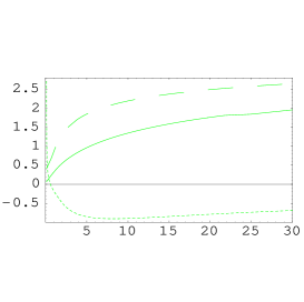
$F_{T}(Q^{2})$
$x_{B}=10^{-3}$	$x_{B}=5\cdot 10^{-4}$	$x_{B}=10^{-5}$
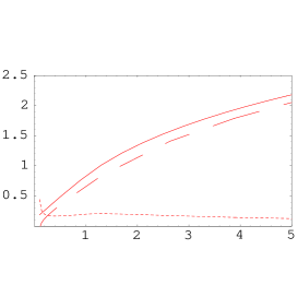
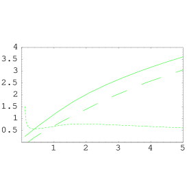
$F_{L}^{D}(Q^{2})$
$x_{B}=10^{-3}$	$x_{B}=5\cdot 10^{-4}$	$x_{B}=10^{-5}$
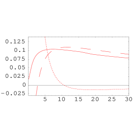
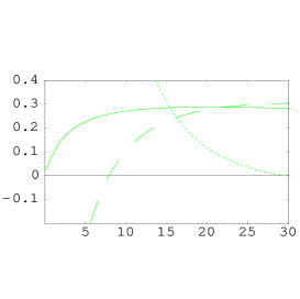
$F_{T}^{D}(Q^{2})$
$x_{B}=10^{-3}$	$x_{B}=5\cdot 10^{-4}$	$x_{B}=10^{-5}$

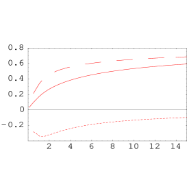
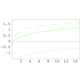
Figure 1: Different twist contributions to the various structure functions for DIS on the proton: leading twist (at high $Q^{2}$) – dashed line, next-to-leading – dotted one, exact structure function – solid curve.

$(a)$	$(b)$

Figure 2: $(a)$ Ratio $F_{L}/F_{T}$ versus $Q^{2}$ for different $x_{B}$, $(b)$ the same for $F_{L}^{D}/F_{T}^{D}$

$(a)$	$(b)$

Figure 3: Scaling of the maxima of ratios $F_{L}/F_{T}$ ($Q^{2}_{max}$) and $F_{L}^{D}/F_{T}^{D}$ ($Q^{2}_{max}(D)$) with $\log_{10}(1/x_{B})$ in $(a)$ the eikonal model, $(b)$ the GW model.

References

- [1] E. Gotsman, E. Levin, U. Maor, L. McLerran, K. Tuchin hep-ph/0007258,
- [2] L.V. Gribov, E.M. Levin and M.G. Ryskin, Phys. Rept. 100:1 (1983).
- [3] A.H. Mueller and J. Qiu, Nucl. Phys. B268:427 (1996).
- [4] L. McLerran and R. Venugopalan, Phys. Rev. D49:2233,3352 (1994), Phys. Rev. D50:2225 (1994), Phys. Rev. D53:458 (1996), Phys. Rev. D59:094002 (1999).
- [5] E. Levin and M.G. Ryskin, Phys. Rep. 189:267 (1990); J.C.Collins and J. Kwiecinski, Nucl. Phys. B335:89 (1990); J. Bartels, J. Blumlein and G. Shuler, Z. Phys. C50:91 (1991); E. Laenen and E. Levin, Ann. Rev. Nucl. Part. Sci. 44:199 (1994) and references therein; A.L. Ayala, M.B. Gay Ducati and E.M. Levin, Nucl. Phys. B493:305 (1997), Nucl. Phys. B510:355 (1998); Yu. Kovchegov, Phys. Rev. D54:5463 (1996); Phys. Rev. D55:5445 (1997), Phys. Rev. D60:034008 (1999); A.H. Mueller, Nucl. Phys. B572:227 (2000), Nucl. Phys. B558:285 (1999); Yu. V. Kovchegov, A.H. Mueller, Nucl. Phys. B529:451 (1998); M. Braun LU-TP-00-06,hep-ph/0001268.
- [6] Yu. V. Kovchegov, Phys. Rev. D60:034008 (1999).
- [7] I. Balitsky Nucl. Phys. B463:1996 (99).
- [8] J. Jalilian-Marian, A. Kovner, L. McLerran and H. Weigert, Phys. Rev. DD55:5414 (1997); J. Jalilian-Marian, A. Kovner and H. Weigert, Phys. Rev. D59:014015 (1999); J. Jalilian-Marian, A. Kovner and H. Weigert, Phys. Rev. D59:014015 (1999); J. Jalilian-Marian, A. Kovner, A. Leonidov and H. Weigert, Phys. Rev. D59:014014,034007 (1999); Erratum-ibid. Phys. Rev. D59:099903 (1999); A. Kovner, J.Guilherme Milhano and H. Weigert, OUTP-00-10P, NORDITA-2000-14-HE, hep-ph/0004014; H. Weigert, NORDITA-2000-34-HE, hep-ph/0004044.
- [9] Yu. V. Kovchegov, Phys. Rev. D61:074018 (2000); E. Levin and K. Tuchin, Nucl. Phys. B573:833 (2000)
- [10] A. Zamolodchikov, B. Kopeliovich and L. Lapidus, JETP Lett. 33:612 (1981); E.M. Levin and M.G. Ryskin, Sov. J. Nucl. Phys. 45:150 (1987); A.H. Mueller, Nucl. Phys. B335:115 (1990).
- [11] A.H. Mueller, Nucl. Phys. B415:373 (1994).
- [12] N.N. Nikolaev and B.G. Zakharov, Z. Phys. C49:607 (1991), plb2604141991; E.M. Levin, A.D. Martin, M.G. Ryskin and T. Teubner, Z. Phys. C74:671 (1997).
- [13] H. Abramowicz, L. Frankfurt and M. Strikman,Surveys High Energ.Phys. bf 11:51 (1997) and references therein; B.Blaettel,G. Baym, L. L. Frankfurt, H. Heiselberg and M. Strikman, Phys. Rev. D47:2761 (1993); A.L. Ayala, M.B. Gay Ducati and E.M. Levin, Nucl. Phys. B493:305 (1997), Nucl. Phys. B510:355 (1998) and references therein; E. Gotsman, E. Levin and U. Maor, Phys. Lett. B403:120 (1997), Nucl. Phys. B493:354 (1997), Nucl. Phys. B464:251 (1996); Yu. V. Kovchegov and L. McLerran, Phys. Rev. D60:054025 (1999).
- [14] E. Gotsman, E. Levin, M. Lublinsky, U. Maor and K. Tuchin, hep-ph/0007261.
- [15] E. Gotsman, E. Levin, M. Lublinsky, U. Maor and K. Tuchin, hep-ph/9911270.
- [16] A.L. Ayala, M.B. Gay Ducati, E.M. Levin, Nucl. Phys. B493:1997 (305).
- [17] A.L. Ayala, M.B. Gay Ducati, E.M. Levin, Nucl. Phys. B511:1998 (355).
- [18] H. Bateman and A. Erdelyi, Higher transcendental functions, v.1, McGraw-Hill, 1953.
- [19] K. Golec-Biernat and M. Wusthoff, Phys. Rev. D59:014017 (1999), Phys. Rev. D60:114023 (1999).
- [20] A.M. Stasto, K. Golec-Biernat and J. Kwiecinski, hep-ph/0007192
- [21] M. Glück, E. Reya and A. Vogt, Z. Phys. C67:433 (1995).
- [22] M. Glück, E. Reya and A. Vogt, Z. Phys. C5:461 (1998).
- [23] J. Bartels, K. Golec-Biernat and K. Peters, hep-ph/0003042.