pNRQCD: CONCEPTS and APPLICATIONS

Abstract

Heavy quark bound state systems, mesons and hybrids, are discussed in the framework of the QCD effective field theory called potential Non-Relativistic QCD.

1 The physical systems

Among all the hadrons, the ones that should be the simplest to analyze are those entirely composed by heavy quarks (and gluons). As it is evident from the spectra (e.g. by comparing the characteristic energy levels splitting with the value of the mass of the quarks in heavy quarkonium), these systems are nonrelativistic. Thus, they can be described in first approximation using a Schrödinger equation with a potential interaction. This amounts to saying that the heavy quark bound state is characterized by three energy scales, hierarchically ordered by the quark velocity $v\ll 1$: the mass $m$ (hard scale), the relative momentum $mv$ (soft scale) and the binding energy $mv^{2}$ (ultrasoft scale). These scales typically get mixed in any Feynman diagram bound state calculation and originate technical complications (the same happens in QED e.g. for positronium). On the other hand, even in a lattice calculation, it is difficult to handle physical systems that possess two very different scales, say $Q\gg q$, since a really demanding relation should then hold for the lattice size $L$ and the lattice step $a$: $L^{-1}\ll q\ll Q\ll a^{-1}$.

In QCD, a further conceptual complication arises due to the existence of a nonperturbative scale, call it $\Lambda_{\rm QCD}$, the scale at which the nonperturbative effects become dominant. For heavy quarks only the hard scale $m$ is surely bigger than $\Lambda_{\rm QCD}$ and can be treated perturbatively. Many attempts have been made to properly consider the effect of the nonperturbative dynamics on the heavy quark energy levels. On the one hand, phenomenological or QCD derived confining potential models have been used inside a Schrödinger equation. Such a picture suffers from many ambiguities, it is strongly model dependent, it consists in a by hand superposition of perturbative and nonperturbative effects, and it leaves out the physics connected to the retardation effects, that’s to say the physics at the ultrasoft (US) scale. On the other hand, the contribution to the Coulombic energy levels due to local condensates has also been evaluated [1]. This correction is of nonpotential type (it is analogue to the Lamb shift effect) and it grows out of control for the excited levels.

Summarizing, the existence of different scales and the nontrivial features related to perturbative (hard scale) and nonperturbative (low scale) effects and to potential and nonpotential contributions, complicate considerably the description of the heavy quark bound states. I will show here how it is possible to take advantage of the existence of this hierarchy of widely separated energy scales to construct QCD effective field theories (EFT) with less and less degrees of freedom. This leads ultimately to a field theory derived quantum mechanical description of these systems. The corresponding EFT is called pNRQCD (potential NonRelativistic QCD) [2, 3]. Here, all the dynamical regimes are organized in a systematic expansion.

2 The QCD effective theories for these systems

The idea is that since the typical scales of a nonrelativistic bound state system are widely separated, it is possible to perform an expansion of one scale in terms of the others. Roughly speaking, first one expands in ${1/m}$ and then one performs an expansion in the inverse of the soft scale, the so called multipole expansion [4, 1, 2, 3]. The effective theory supplies us with the procedure to make this expansion consistent with the ultraviolet behaviour of QCD and consistent with a systematic power counting in the small expansion parameter $v$. As I will explain below, it depends on the physical system in consideration and on the actual position of $\Lambda_{\rm QCD}$ into this hierarchy of scales, if it is possible or not to take advantage of the further simplification of performing the calculations in a perturbative expansion in $\alpha_{s}$.

2.1 NRQCD

First we pass from QCD to NRQCD by integrating out the hard scale $m$. This involves performing an expansion in ${1/m}$, which, in the two-fermions sector is of the type of the Foldy-Wouthuysen transformation. Since we are modifying the ultraviolet behaviour of the theory, matching coefficients and new operators have to be added in order to mock up the effects of heavy particles and high energy modes into the low energy EFT. In this case, since the scale of the mass of the heavy quark is perturbative, the scale $\mu$ of the matching from QCD to NRQCD, $mv<\mu<m$, lies also in the perturbative regime. Then, the hard scale is integrated out by comparing on shell amplitudes, order by order in ${1/m}$ and in $\alpha_{s}$, in QCD and in NRQCD. The difference is encoded into the matching coefficients that typically depend non-analytically on the scale which has been integrated out, in this case $m$. We work here in dimensional regularization, $\overline{MS}$ scheme, and with quark pole masses. Up to order ${1/m^{2}}$ the Lagrangian of NRQCD [5] reads:

$$\ L=\psi^{\dagger}\left(iD_{0}+c_{2}{{\bf D}^{2}\over 2m}+c_{4}{{\bf D}^{4}\over 8m^{3}}+c_{F}g{{\bf S}\cdot{\bf B}\over m}+c_{D}g{{\bf D}\cdot{\bf E}-{\bf E}\cdot{\bf D}\over 8m^{2}}\right.$$ (1)

$$\left.+ic_{S}g{{\bf S}\cdot({\bf D}\times{\bf E}-{\bf E}\times{\bf D})\over 4m^{2}}\right)\psi+\hbox{\, antiquark terms}+\hbox{\, terms with light quarks}$$

$$-{b_{1}\over 4}F_{\mu\nu}^{a}F^{a\,\mu\nu}+{b_{2}\over m^{2}}F_{\mu\nu}^{a}D^{2}F^{a\,\mu\nu}+{b_{3}\over m^{2}}gf_{abc}F_{\mu\nu}^{a}F_{\mu\alpha}^{b}F_{\nu\alpha}^{c}$$

$$+{d_{1}\over m^{2}}\psi^{\dagger}\psi\chi^{\dagger}\chi+{d_{2}\over m^{2}}\psi^{\dagger}{\bf S}\psi\chi^{\dagger}{\bf S}\chi+{d_{3}\over m^{2}}\psi^{\dagger}T^{a}\psi\chi^{\dagger}T^{a}\chi+\!{d_{4}\over m^{2}}\psi^{\dagger}T^{a}{\bf S}\psi\chi^{\dagger}T^{a}{\bf S}\chi,$$

$\psi$ and $\chi$ being respectively the quark and the antiquark field; $D^{\mu}$ is the covariant derivative, ${\bf E}$ and ${\bf B}$ are chromoelectric and chromomagnetic fields, $F^{\mu\nu}$ is the gluon field strength, ${\bf S}$ is the total spin, $T^{a}$ is the color generator, $g$ is the coupling constant. $c_{i},b_{i},d_{i}$ are matching coefficients. They depend on $\mu$ and $m$ and are known in the literature at a different level of precision. The $\mu$ dependence in the matching coefficients cancels against the $\mu$ dependence of the operators in the Lagrangian. The gluonic part in the third line comes from the vacuum polarization while the last line contains four quark operators.

Many applications of NRQCD have been made both in lattice calculations and in the continuum, see e.g. [5, 6]. Here, however I just introduced NRQCD as a step towards pNRQCD. I recall in fact that in NRQCD two dynamical scales are still present, $mv$ and $mv^{2}$. These scales get entangled and obscure the power counting, i.e. the matrix elements of the operators in (1) do not have a unique power counting but they also contribute to subleading orders in $v$. In the next section I will show how it is possible to integrate out also the momentum scale, obtaining an effective theory at the ultrasoft scale. This effective theory is called pNRQCD.

2.2 pNRQCD

When we integrate out the soft scale $mv$, there are two possible situations depending on the relative position of $\Lambda_{\rm QCD}$ with respect to the other scales. If $\Lambda_{\rm QCD}$ is smaller than $mv$, then also the matching from NRQCD to pNRQCD may be performed in perturbation theory. If $\Lambda_{\rm QCD}\simeq mv$ the soft scale is already nonperturbative and the matching to pNRQCD has to be performed avoiding any expansion in $\alpha_{s}$. Roughly speaking, we can say that the lowest excitations of quarkonium belong to the first situation while the excited states belong to the second situation. Indeed, the typical radius of the bound state is proportional to the inverse of the soft scale $r\simeq 1/mv$ and thus for the lowest states the condition $mv\ll\Lambda_{\rm QCD}$ may be fulfilled. In Fig.1 I present the typical radius of various mesons against the curve of a phenomenological potential that displays a nonperturbative (linear) behaviour around 0.2 fm. In the following I will discuss both situations.

b

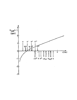
Figure 1: $r_{q\bar{q}}$ of various mesons vs the Cornell potential, from⁷.

3 pNRQCD for $mv\gg\Lambda_{\rm QCD}$

We denote by ${\bf R}\equiv{({\bf x}_{1}+{\bf x}_{2}})/2$ the center of mass of the $Q\bar{Q}$ system and by ${\bf r\equiv{\bf x}_{1}-{\bf x}_{2}}$ the relative distance. The matching to pNRQCD is perturbative. At the scale of the matching $\mu^{\prime}$ ($mv\gg\mu^{\prime}\gg mv^{2},\Lambda_{\rm QCD}$) we have still quarks and gluons. The effective degrees of freedom are: $Q\bar{Q}$ states (that can be decomposed into a singlet $S({\bf R},{\bf r},t)$ and an octet $O({\bf R},{\bf r},t)$ under color transformations) with energy of order of the next relevant scale, $O(\Lambda_{QCD},mv^{2})$ and momentum ${\bf p}$ of order $O(mv)$, plus ultrasoft gluons $A_{\mu}({\bf R},t)$ with energy and momentum of order $O(\Lambda_{\rm QCD},mv^{2})$. Notice that all the gluon fields are multipole expanded. The Lagrangian is then an expansion in the small quantities ${p/m}$, ${1/rm}$ and in $O(\Lambda_{\rm QCD},mv^{2})\times r$.

3.1 The pNRQCD Lagrangian

At the next-to-leading order (NLO) in the multipole expansion, i.e. at $O(r)$, we get [2, 3]

$$L^{(1)}_{\rm pNRQCD}=-{1\over 4}F_{\mu\nu}^{a}F^{\mu\nu\,a}+{\rm Tr}\left\{{\rm S}^{\dagger}\left(i\partial_{0}-{{\bf p}^{2}\over m}-V_{s}-\sum_{n=1}{V^{(n)}_{s}\over m^{n}}\right){\rm S}\right\}$$ (2)

$$+{\rm Tr}\left\{{\rm O^{\dagger}}\left(i{D_{0}}-{{\bf p}^{2}\over m}-V_{o}-\sum_{n=1}{V^{(n)}_{o}\over m^{n}}\right){\rm O}\right\}$$

$$+{g}V_{A}{\rm Tr}\left\{{\rm O^{\dagger}}{\bf r}\cdot{\bf E}\,{\rm S}+{\rm S^{\dagger}}{\bf r}\cdot{\bf E}\,{\rm O}\right\}+{g}{V_{B}\over 2}{\rm Tr}\left\{{\rm O^{\dagger}}{\bf r}\cdot{\bf E}\,{\rm O}+{\rm O^{\dagger}}{\rm O}{\bf r}\cdot{\bf E}\right\}.$$

The matching coefficients $V_{j}$ are functions of $\mu,\mu^{\prime},{\bf r},{\bf p},{\bf S}_{1},{\bf S_{2}}$. The equivalence of pNRQCD to NRQCD, and hence to QCD, is enforced by requiring the Green functions of both effective theories to be equal (matching). In practice, appropriate off shell amplitudes are compared in NRQCD and in pNRQCD, order by order in the expansion in $1/m$, $\alpha_{s}$ and in the multipole expansion. The difference is encoded in these potential-like matching coefficients that depend non-analytically on the scale that has been integrated out (in this case ${\bf r})$. Recalling that ${\bf r}\simeq 1/mv$ and that the operators count like the next relevant scale, $O(mv^{2},\Lambda_{\rm QCD})$, to the power of the dimension, it follows that each term in the pNRQCD Lagrangian has a definite power counting. This feature makes $L_{\rm pNRQCD}$ the most suitable tool for a bound state calculation: being interested in knowing the energy levels up to some power $v^{n}$, we just need to evaluate the contributions of this size in the Lagrangian. The singlet sector of the Lagrangian would give rise to equations of motion of the Schrödinger type, while the last line of (2) contains retardation (or nonpotential) effects that start at the NLO in the multipole expansion. At this order the nonpotential effects come from the singlet-octet interaction mediated by a ultrasoft chromoelectric field.

Summarizing, pNRQCD is equivalent to QCD, it has potential terms, thus embracing potential models, and it has ultrasoft gluons incorporated in a second-quantized, gauge-invariant and systematic way. Moreover, the power counting in $v$ is explicit and subsequent corrections both in the $1/m$ expansion as in the multipole expansion can be added systematically. Hard and soft effects are separated from the ultrasoft (low-energy) effects.

The Feynman rules corresponding to the Lagrangian (2) are shown in Fig.2.

At zero order in the multipole expansion the singlet and the octet decouple and their equations of motion turn out to be Schrödinger-like. Then, the first question comes: is the singlet matching coefficient $V_{s}$ equal to the static heavy quark potential? The answer depends on the actual ratio of $mv^{2}$ and $\Lambda_{\rm QCD}$. In the EFT language the potential is defined upon the integration of all the scales up to the ultrasoft scale $mv^{2}$. We can imagine two different situations: if $\Lambda_{\rm QCD}{\ \lower-1.2pt\vbox{\hbox{\hbox to0.0pt{$<$\hss}\lower 6.0pt\vbox{\hbox{$\sim$}}}}\ }mv^{2}$, then $V_{s}$ is the static heavy quark potential; if $mv\ll\Lambda_{\rm QCD}\ll mv^{2}$, then we have to integrate out also $\Lambda_{\rm QCD}$ in order to get the potential. In this integration the potential acquires short range nonperturbative contributions as I will show in Sec.3.3.

A second interesting question is what is the relation between $V_{s}$ and the energy $E_{s}$ between quark static sources, which is defined as

$$E_{s}(r)=\displaystyle\lim_{T\to\infty}{i\over T}\ln\langle W_{\Box}\rangle,$$ (3)

being $W_{\Box}$ the static Wilson loop of size ${\bf r}\times T$, and the symbol $\langle~{}~{}\rangle$ being the average over the gauge fields. $E_{s}$ is often used as a static potential inside the Schrödinger equation, assuming that the Born-Oppenheimer approximation holds. We answer these questions by performing explicitly the singlet matching at order $1/m^{0}$ and at the NLO in the multipole expansion.

b

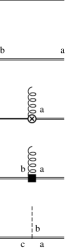
Figure 2: Propagators and vertices of the pNRQCD Lagrangian (at order $1/m^{0}$ and at the NLO in the multipole expansion).

3.2 The matching procedure: the singlet ($\Lambda_{\rm QCD}{\ \lower-1.2pt\vbox{\hbox{\hbox to0.0pt{$<$\hss}\lower 6.0pt\vbox{\hbox{$\sim$}}}}\ }mv^{2}$)

The matching can be done once the interpolating fields for $S$ and $O^{a}$ have been identified in NRQCD. The former need to have the same quantum numbers and the same transformation properties as the latter. The correspondence is not one-to-one. Given an interpolating field in NRQCD, there is an infinite number of combinations of singlet and octet wave-functions with ultrasoft fields, which have the same quantum numbers and, therefore, have a non vanishing overlap with the NRQCD operator. However, the operators in pNRQCD can be organized according to the counting of the multipole expansion. For instance, for the singlet we have

$$\chi^{\dagger}({\bf x}_{2},t)\phi({\bf x}_{2},{\bf x}_{1};t)\psi({\bf x}_{1},t)=Z^{1/2}_{s}(r)S({\bf R},{\bf r},t)+Z^{1/2}_{E,s}(r)r\,{\bf r}\cdot{\bf E}^{a}({\bf R},t)O^{a}({\bf R},{\bf r},t)+\dots,$$ (4)

and for the octet

$$\!\!\!\chi^{\dagger}({\bf x}_{2},t)\phi({\bf x}_{2},{\bf R};t)T^{a}\phi({\bf R},{\bf x}_{1};t)\psi({\bf x}_{1},t) = Z^{1/2}_{o}(r)O^{a}({\bf R},{\bf r},t)$$

$$+ Z^{1/2}_{E,o}(r)r\,{\bf r}\cdot{\bf E}^{a}({\bf R},t)S({\bf R},{\bf r},t)+\dots,$$

$\phi({\bf y},{\bf x};t)\equiv{\rm P}\exp\{ig\int_{0}^{1}\!\!ds\,({\bf y}-{\bf x})\cdot{\bf A}({\bf x}-s({\bf x}-{\bf y}),t)\}$, $Z_{i}$ being normalization factors. These operators guarantee a leading overlap with the singlet and the octet wave-functions respectively. Higher order corrections are suppressed in the multipole expansion. The expressions for the octet can be made manifestly gauge-invariant by inserting a magnetic field in place of the pure color matrix. The fact that the matching can be done in a completely gauge-invariant way enables us to generalize pNRQCD to the case in which $\Lambda_{\rm QCD}\simeq mv$, i.e. to the nonperturbative matching, cf. Sec. 5.

Now, in order to get the singlet potential, we compare 4-quark Green functions. From (4), we take in NRQCD

$$I=\delta^{3}({\bf x}_{1}-{\bf y}_{1})\delta^{3}({\bf x}_{2}-{\bf y}_{2})\langle W_{\Box}\rangle,$$ (6)

and we equate (6) to the singlet propagator in pNRQCD at NLO in the multipole expansion (cf. Fig. 3 for a diagrammatic representation)

$$\!\!\!\!\!\!\!\!\!I=Z_{s}(r)\delta^{3}({\bf x}_{1}-{\bf y}_{1})\delta^{3}({\bf x}_{2}-{\bf y}_{2})e^{-iTV_{s}(r)}\times$$ (7)

$$\!\!\!\!\!\!\!\!\!\!\!\!\Bigg{(}1-{g^{2}\over N_{c}}T_{F}V_{A}^{2}(r)\int_{-T/2}^{T/2}\!\!\!dt\int_{-T/2}^{t}\!\!\!dt^{\prime}e^{-i(t-t^{\prime})(V_{o}-V_{s})}\langle{\bf r}\cdot{\bf E}^{a}(t)\phi(t,t^{\prime})^{\rm adj}_{ab}{\bf r}\cdot{\bf E}^{b}(t^{\prime})\rangle\Bigg{)},$$

where $\phi^{\rm adj}$ is a Schwinger (straight-line) string in the adjoint representation and fields with only temporal argument are evaluated in the centre-of-mass coordinate. From here one gets the singlet static potential $V_{s}$ (and the singlet wave-function normalization $Z_{s}$):

$$V_{s}(r)=E_{s}(r)\big{|}_{\rm 2-loop+NNNLL}+C_{F}{\alpha_{\rm s}\over r}{\alpha^{3}_{\rm s}\over\pi}{C_{A}^{3}\over 12}\ln{C_{A}\alpha_{\rm s}\over 2r\mu^{\prime}},$$ (8)

where $E_{s}$ has been defined in Eq. (3) We note that $V_{s}$ and $E_{s}$ would coincide in QED and that therefore the effect we are studying here is a genuine QCD feature.

b

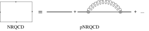
Figure 3: The matching between the Wilson loop in NRQCD and the singlet propagator in pNRQCD.

The leading log contributions to the NNNLO arise from three loops diagrams that are infrared divergent. The final result reads

$$V_{s}(r,\mu^{\prime}) = -C_{F}{\alpha_{V}(r,\mu^{\prime})\over r},$$ (9)

$$\alpha_{V}(r,\mu^{\prime}) = \alpha_{\rm s}(r)\Big{[}1+\tilde{a}_{1}\alpha_{\rm s}(r)+\tilde{a}_{2}(\alpha_{\rm s}(r))^{2}+{\alpha_{\rm s}^{3}\over\pi}{C_{A}^{3}\over 12}\ln{\mu^{\prime}r}\Big{]}.$$

This is the LL three loop evaluation of the static heavy quark potential in the case $\Lambda_{\rm QCD}{\ \lower-1.2pt\vbox{\hbox{\hbox to0.0pt{$<$\hss}\lower 6.0pt\vbox{\hbox{$\sim$}}}}\ }mv^{2}$. The one loop and two-loop contributions come from [8] and the three loop LL from [9].

This situation is expected to hold for toponium and for the bottomonium (charmonium?) ground state. The explicit $\mu^{\prime}$ dependence of $V_{s}$ originates from the fact that the US degrees of freedom (which have the same scale of the kinetic energy and therefore do not belong to the potential) have been explicitly subtracted out from the static Wilson loop. This fact is not surprising if we understand the heavy quarkonium potential as a matching coefficient of pNRQCD. As a consequence even in a purely perturbative regime the static heavy quarkonium potential (as well as $\alpha_{V}$) turns out to be an infrared sensitive quantity. In this situation nonperturbative effects are only of non-potential nature and appear in the form of local (à la Leutwyler–Voloshin) or nonlocal condensates. When calculating any physical observable, the $\mu^{\prime}$ dependence cancels against $\mu^{\prime}$-dependent contributions coming from the dynamical US gluons [10].

In a similar way, by matching appropriate Green functions, we can get the octet matching potential $V_{o}$ and the other matching potentials [3, 10].

3.3 The singlet potential in the situation $mv\gg\Lambda_{\rm QCD}\gg mv^{2}$

Since in this situation there is a physical scale ($\Lambda_{\rm QCD}$) above the US scale, a potential can be properly defined only once this scale has been integrated out. At the NLO in the multipole expansion we get

$$\!\!\!\!\!\!\!\!\!\!\!\!\!\!\!V_{s}(r)=-C_{F}{\alpha_{V}(r,\mu^{\prime})\over r}-i{g^{2}\over N_{c}}T_{F}V_{A}^{2}(r){r^{2}\over 3}\int_{0}^{\infty}\!\!\!\!dte^{-it(V_{o}-V_{s})}\langle{{\bf E}^{a}}(t)\phi(t,0)^{\rm adj}_{ab}{\bf E}^{b}(0)\rangle(\mu^{\prime}).$$

(10)

Therefore, the heavy quarkonium static potential $V_{s}$ is given in this situation by the sum of the purely perturbative piece calculated in Eq. (9) and a new term carrying also nonperturbative contributions (contained into non-local gluon field correlators). This last one can be organized as a series of power of $r^{n}$ by expanding $\exp\{-it(V_{o}-V_{s})\}=1-it(V_{o}-V_{s})+\dots$ (since $t\simeq 1/\Lambda_{\rm QCD}$, $V_{o}-V_{s}\simeq mv^{2}$). Typically the nonperturbative piece of Eq. (10) absorbs the $\mu^{\prime}$ dependence of $\alpha_{V}$ so that the resulting potential $V_{s}$ is now scale independent.
We notice that the leading nonperturbative term could be as important as the perturbative potential once the power counting is established and, if so, it should be kept exact when solving the Schrödinger equation. In Table 1 we summarize the different kinematic situations.

b $mv$ $mv^{2}$ potential ultrasoft corrections $\gg\Lambda_{\rm QCD}$ $\gg\Lambda_{\rm QCD}$ perturbative local condensates $\gg\Lambda_{\rm QCD}$ $\sim\Lambda_{\rm QCD}$ perturbative non-local condensates $\gg\Lambda_{\rm QCD}$ $\ll\Lambda_{\rm QCD}$ perturbative + No US (if light quarks short-range nonpert.     are not considered)

Table 1: Summary of the different kinematic situations.

We can also consider Eq.(10) in the limit of static sources. In this case there are no dynamical scales involved and therefore in the short range we have $\exp{\{-it(V_{o}-V_{s})\}}\langle{{\bf E}^{a}}(t)\phi(t,0)^{\rm adj}_{ab}{\bf E}^{b}(0)\rangle$ $\simeq$ $\exp{\{-it(V_{o}-V_{s})\}}\langle E(0)^{2}\rangle$. This gives

$$E_{s}(r)\simeq-C_{\rm F}{\alpha_{\rm V}(r,{\alpha_{s}\over r})\over r}-{r^{3}\over 3}{g^{2}\over N_{c}^{2}\alpha_{s}}\langle E^{2}(0)\rangle$$ (11)

which coincides with [13].

4 Application of pNRQCD ($\Lambda_{\rm QCD}<mv$)

• Quarkonium spectrum at leading-log of NNNLO
  The complete leading-log terms of the NNNLO corrections to pNRQCD have been calculated [10]. As a byproduct the leading logs at $O(m\alpha_{s}^{5})$ in the heavy quarkonium spectrum have been obtained. When $\Lambda_{\rm QCD}\ll m\alpha_{s}^{2}$, these leading logs give the complete $O(m\alpha_{s}^{5}\ln\alpha_{s})$ corrections to the heavy quarkonium spectrum (plus the nonpotential contributions coming from local condensates) [10]. The result is important at least for $t\bar{t}$ production and $\Upsilon$ physics. In the first case this result is a first step towards the goal of reaching a 100 MeV sensitivity on the top quark mass from the $t\bar{t}$ cross section near threshold to be measured at future linear colliders. In the second case it will improve our knowledge on the $b$ mass. In both cases the LL contributions of NNNLO have been found to be relevant [11, 12].

• Renormalons
  The infrared sensitivity of the static potential can also be expressed in the renormalons language, i.e. we can say that $V_{s}$, as defined in Eq.(9), suffers from IR renormalons ambiguities with the following structure

  $$V_{s}(r)|_{\rm IR\,ren}=C_{0}+C_{2}r^{2}+\dots$$ (12)

  The constant $C_{0}\sim\Lambda_{\rm QCD}$ is known to be cancelled by the pole mass IR renormalon ($2m_{\rm pole}|_{\rm IR\,ren}=-C_{0})$. While Eq. (10) provides us with the explicit expression for the operator which absorbs the $C_{2}\sim\Lambda_{\rm QCD}^{3}$ ambiguity [3]. The renormalon cancellation issue plays an important role in quarkonium phenomenology [14].

• Hybrids and gluelumps
  pNRQCD gives model independent predictions on the behaviour of the hybrid static potentials. In particular it predicts for these potentials an octet behaviour at very short distances and it correctly states all the degeneration patterns in the small $r$ region [3]. Moreover, it allows to relate the mass of the gluelumps to the correlation lengths of some nonlocal vacuum field strength correlators [15, 3].

• Quarkonium scattering, Van Der Waals forces, Quarkonium Production. Work is in progress on these applications.

• Renormalization group improvement
  Up to now, it has been performed at the level of the static potential [16].

5 pNRQCD for $\Lambda\simeq mv$

In this case the potential interaction is dominated by nonperturbative effects. This is the most interesting situation, in which most of the mesons lie (cf. Fig.1).

A large effort has been made in the last decades in order to obtain from QCD the nonperturbative potentials in the Wilson loop approach [17, 18, 6]. pNRQCD allows us to obtain via a nonperturbative matching all the nonperturbative potentials [19]. From this respect I want to discuss few concepts and results.

In pNRQCD a potential picture for heavy quarkonium emerges at the leading order in the US expansion under the condition that the matching between NRQCD and pNRQCD can be performed within an expansion in $1/m$. The gluonic excitations (hybrids and glueballs) that form a gap of order $\Lambda_{\rm QCD}$ with respect to the quarkonium state can be integrated out and the potentials follow in an unambiguous and systematic way from the nonperturbative matching to pNRQCD. Thus, we recover the quark model from pNRQCD. The US degrees of freedom in this case are not coloured gluons but US gluonic excitations between heavy quarks and pions. They can be systematically included and may eventually affect the leading potential picture. Let us consider for instance the singlet matching potential. Disregarding the US corrections, we have the identification

$$V_{s}(r)=\lim_{T\to\infty}{i\over T}\ln\langle W(r\times T)\rangle.$$

US corrections to this formula are due to pions and US gluonic excitations between heavy quarks, and may be included in the same way as the effects due to US gluons have been included in the perturbative situation through Eq. (8).

The complete $1/m^{2}$ potential has been calculated along these lines [19]. There are many appealing and interesting features of this procedure. The matching calculation is performed in the way of the quantum mechanical perturbation theory on the QCD Hamiltonian (where perturbations are counted in orders of $1/m$ and not of $\alpha_{s}$) and only at a later stage the relation with the Wilson loop and field insertions is established. This allows us to have a control on the Fock states of the problem and on the contributions coming from gluonic excitations in the intermediate states. At the end, all the expressions are again given in terms of Wilson loops, which can be evaluated on the lattice or in QCD vacuum models [18]. The potentials turn out to be naturally factorized in a hard part (the matching coefficients at the hard scales inherited by pNRQCD from NRQCD) and a low energy part (the Wilson loops expressions). The power counting may turn out to be quite different from the perturbative (QED-like) situation.

6 Conclusion and outlook

I have shown that it is possible to construct systematically and within a controlled expansion an effective theory of QCD, which describes heavy quark bound states. All known perturbative and nonperturbative regimes (potential, nonpotential), are dynamically present in the theory, which is equivalent to QCD. I have presented many applications of pNRQCD in the situation $\Lambda_{\rm QCD}\ll mv$. In the situation $\Lambda_{\rm QCD}\simeq mv$, I have discussed how pNRQCD allows us to systematically factorize the nonperturbative heavy quark dynamics.

References

References

- [1] M. B. Voloshin, Nucl. Phys. B 154, 365 (1979); H. Leutwyler, Phys. Lett. B 98, 447 (1981)
- [2] A. Pineda and J. Soto, Nucl. Phys. B (Proc. Suppl.) 64, 428 (1998);
- [3] N. Brambilla, A. Pineda, J. Soto, A. Vairo, Nucl. Phys. B 566, 275 (2000).
- [4] M.B. Voloshin, Yad. Fiz. 43, 1571 (1986); P. Labelle, Phys. Rev. D 58, 093013 (1998); M. Beneke and V. A. Smirnov, Nucl. Phys. B 522, 321 (1998); M. E. Luke, A. V. Manohar and I. Z. Rothstein, Phys. Rev. D61, 074025 (2000).
- [5] W. E. Caswell and G. P. Lepage, Phys. Lett. B 167, 437 (1986); G. T. Bodwin, E. Braaten and G. P. Lepage, Phys. Rev. D 51, 1125 (1995); A. V. Manohar, Phys. Rev. D 56, 230 (1997); A. Pineda and J. Soto, Phys. Rev. D 58, 114011 (1998).
- [6] N. Brambilla and A. Vairo, hep-ph/9904330; G. S. Bali, hep-ph/0001312.
- [7] S. Godfrey and N. Isgur, Phys. Rev. D 32, 189 (1985).
- [8] A. Billoire, Phys. Lett. B 92, 343 (1980); Y. Schröder, Phys. Lett. B 447, 321 (1999); M. Peter, Phys. Rev. Lett. 78, 602 (1997).
- [9] N. Brambilla, A. Pineda, J. Soto and A. Vairo, Phys. Rev. D 60, 091502 (1999); A. Vairo, Nucl. Phys. Proc. Suppl. 86, 521 (2000).
- [10] N. Brambilla, A. Pineda, J. Soto, A. Vairo, Phys. Lett. B 470, 215 (1999); B. A. Kniehl and A. A. Penin, Nucl. Phys. B 563, 200 (1999).
- [11] B. A. Kniehl, A. A. Penin, Nucl. Phys. B 577, 197 (2000).
- [12] F. J. Yndurain, hep-ph/0008007, hep-ph/0002237, hep-ph/9910399.
- [13] C. A. Flory, Phys. Lett. B 113, 263 (1982).
- [14] M. Beneke, Phys. Lett. B 434, 115 (1998); A.H. Hoang, Z. Ligeti and A. Manohar, Phys. Rev. Lett. 82, 277 (1999); N. Brambilla and A. Vairo, hep-ph/0002075; Y. Kiyo, Y. Sumino, hep-ph/0007251.
- [15] N. Brambilla and A. Vairo, hep-ph/0004192; N. Brambilla, Nucl. Phys. B (Proc. Suppl.) 86, 389 (2000).
- [16] A. Pineda and J. Soto, hep-ph/0007197.
- [17] K. G. Wilson, Phys. Rev. D 10, 2445 (1974); E. Eichten and F. L. Feinberg, Phys. Rev. D 23, 2724 (1981); D. Gromes, Z. Phys. C 26, 401 (1984). A. Barchielli, E. Montaldi and G. M. Prosperi, Nucl. Phys. B 296, 625 (1988); A. Barchielli, N. Brambilla, G. Prosperi, Nuovo Cimento 103 A, 59 (1990); Y. Chen, Y. Kuang and R. J. Oakes, Phys. Rev. D 52, 264 (1995);G. S. Bali, A. Wachter and K. Schilling, Phys. Rev. D 56, 2566 (1997); N. Brambilla and A. Vairo, Nucl. Phys. B (Proc. Suppl.) 74, 201 (1999); N. Brambilla, hep-ph/9809263
- [18] N. Brambilla and A. Vairo, Phys. Rev. D 55, 3974 (1997); N. Brambilla, P. Consoli and G. M. Prosperi, Phys. Rev. D 50, 5878 (1994).
- [19] N. Brambilla, A. Pineda, J. Soto and A. Vairo, hep-ph/0002250; A. Pineda and A. Vairo, HD-THEP-00-31, CERN-TH/2000-197.