A chiral crystal in cold QCD matter at intermediate densities?

Abstract

The analogue of Overhauser (particle-hole) pairing in electronic systems (spin-density waves with non-zero total momentum $Q$) is analyzed in finite-density QCD for 3 colors and 2 flavors, and compared to the color-superconducting BCS ground state (particle-particle pairing, $Q$=0). The calculations are based on effective nonperturbative four-fermion interactions acting in both the scalar diquark as well as the scalar-isoscalar quark-hole (’$\sigma$’) channel. Within the Nambu-Gorkov formalism we set up the coupled channel problem including multiple chiral density wave formation, and evaluate the resulting gaps and free energies. Employing medium-modified instanton-induced ’t Hooft interactions, as applicable around $\mu_{q}\simeq 0.4$ GeV (or 4 times nuclear saturation density), we find the ’chiral crystal phase’ to be competitive with the color superconductor.

I Introduction

The understanding of QCD under extreme conditions is among the main frontiers in strong interaction physics. In particular, the finite-density and zero-temperature regime has reattracted considerable attention lately, after it has been realized that early perturbative estimates for color-superconducting gaps at large chemical potential are exceeded by up to two orders of magnitude towards smaller densities [1, 2, 3, 4]. Such BCS-type pairing energies are in fact comparable to the (’constituent’) quark mass gap in the QCD vacuum, $M_{q}\simeq$ 0.35-0.4 GeV, and have triggered new interest in observable consequences of quark matter formation within the core of neutron stars (unfortunately, in high energy heavy-ion collision large entropy production renders the access to this regime unlikely).

The focus on the occurrence of various superconducting phases is motivated by the standard BCS instability of the Fermi surface for arbitrarily weak particle-particle ($p$-$p$) interactions. Under certain conditions, however, the particle-hole ($p$-$h$) channel might also become competitive. Here, a kinematic singularity in the corresponding Greens function only develops in (effectively) 1+1 dimensional systems, and at a total pair momentum of $Q=2p_{F}$ ($p_{F}$: Fermi momentum), known as Peierls instability [5]. In higher dimensions it can nevertheless be relevant provided the interaction is strong enough. One variant of $p$-$h$ instabilities are ’spin-density waves’ as originally proposed by Overhauser [6] for specific electronic materials (for a review see [7]). The analogue in the context of QCD, so called ’chiral density waves’, has first been discussed by Deryagin et al. [8]. Using perturbative one-gluon exchange (OGE) at asymptotically high densities it was shown that the Overhauser-type pairing prevails over the BCS instability in the $N_{c}\to\infty$ limit ($N_{c}$: number of colors). This is due to the fact that the BCS bound states, being color non-singlet, are dynamically suppressed by 1/$N_{c}$ as compared to the (colorless) Overhauser ones. More recently, Shuster and Son [9] revisited this mechanism for finite $N_{c}$ and including Debye screening in the gluon propagator. As a result, the chiral density wave dominates only for a very large number of colors, $N_{c}={\cal O}(10^{3})$. These findings have been confirmed in an analysis of coupled BCS/Overhauser equations using different arguments [10]. One concludes that instabilities in the $p$-$h$ channel are not relevant for real QCD at asymptotic densities.

The situation, however, can be very different if the interaction strength between the quarks is substantially increased (to be referred to below as the strong coupling regime). A well-known example is the Nambu-Jona Lasinio (NJL) description of chiral symmetry breaking in the QCD vacuum (associated with the constituent quark mass gap and the build-up of the chiral condensate), which requires a (minimal) critical coupling to occur. At finite density, the same (attractive) interaction is operative in the scalar-isoscalar $p$-$h$ channel. It’s coupling strength is in fact augmented by a factor of $(N_{c}-1)$ over the (most attractive) scalar diquark channel. On the other hand, geometric factors act in its disfavor: unlike the BCS gap, which uniformly covers the entire Fermi surface, the chiral density wave appears in form of ‘patches’, their number depending on the symmetry of the presumed crystal. The purpose of the present paper is to study the interplay between Overhauser and BCS pairing, including different crystal structures, within the strong coupling regime. The focus is thus on quark matter at intermediate densities, i.e., large enough for the system to be in the quark phase, but small enough to support nonperturbative interactions. This should roughly correspond to chemical potentials in the range $\mu_{q}\simeq$ 0.4-0.6 GeV, translating into baryon densities of 3.5-12 $\rho_{0}$ (where $\rho_{0}$=0.16 fm^-3 denotes normal nuclear matter density).

The article is organized as follows. In Sect. II we start by introducing the Nambu-Gorkov type matrix propagator formalism that will subsequently be applied to obtain the gap equations for the coupled BCS-Overhauser problem; special attention is given to the single-quark spectra in the Overhauser ground state. In Sect. III we solve these equations using the aforementioned variants of nonperturbative interactions, i.e., somewhat schematic NJL-type as well as microscopic instanton-induced forces, for the slightly idealized case of two massless flavors and three colors. In Sect. IV we summarize and discuss the relevance of our results for real QCD.

II Nambu-Gorkov Formalism and Coupled Gap Equations

A BCS Pairing

A standard framework to address multiple instabilities in interacting many-body systems is provided by the Nambu-Gorkov formalism. Here, propagators are constructed as matrices combining all potential condensate channels via off-diagonal elements (see, e.g., ref. [13]), which automatically incorporates the interplay/coexistence of the various phases.

For the familiar BCS case one adopts the following ansatz for the full propagator:

$$\hat{G}_{BCS}(k_{0},\vec{k},\Delta;\mu_{q})=\left(\begin{array}[]{cc}\langle c_{k\uparrow}~{}c^{\dagger}_{k\uparrow}\rangle&\langle c_{k\uparrow}~{}c_{-k\downarrow}\rangle\\ \langle c^{\dagger}_{-k\downarrow}~{}c^{\dagger}_{k\uparrow}\rangle&\langle c^{\dagger}_{-k\downarrow}~{}c_{-k\downarrow}\rangle\end{array}\right)\ \equiv\left(\begin{array}[]{cc}G(k_{0},\vec{k},\Delta)&\bar{F}(k_{0},\vec{k},\Delta)\\ F(k_{0},\vec{k},\Delta)&\bar{G}(k_{0},-\vec{k},\Delta)\end{array}\right)\ .$$ (1)

The gap equation is then derived by formulating the pertinent Dyson equation,

$$\hat{G}_{BCS}=\left[\hat{G}_{0}^{-1}-\hat{\Delta}\right]^{-1}=\left(\begin{array}[]{cc}{G}_{0}^{-1}&\bar{\Delta}\\ \Delta&\bar{G}_{0}^{-1}\end{array}\right)^{-1}\ ,$$ (2)

which has the formal solution

$$\hat{G}_{BCS}=\frac{1}{G_{0}^{-1}\bar{G}_{0}^{-1}-\Delta\bar{\Delta}}\left(\begin{array}[]{cc}\bar{G}_{0}^{-1}&-{\Delta}\\ -\bar{\Delta}&G_{0}^{-1}\end{array}\right)\ ,$$ (3)

where

$$\Delta=(-i)\ \alpha_{pp}\int\frac{d^{4}p}{(2\pi)^{4}}\ F(p_{0},\vec{p},\Delta)$$ (4)

represents the (off-diagonal) ’selfenergy’ contribution induced by $p$-$p$ pairing (with an appropriate 4-fermion coupling constant $\alpha_{pp}$), and

$$G_{0} = \frac{1}{k_{0}-\epsilon_{k}+i\delta_{\epsilon_{k}}}$$ (5)

$$\bar{G}_{0} = \frac{1}{k_{0}+\epsilon_{k}+i\delta_{\epsilon_{k}}}$$ (6)

are the free particle propagator and its conjugate at finite chemical potential (with $\epsilon_{k}=\omega_{k}-\mu_{q}$ and infinitesimal $\delta_{\epsilon_{k}}=|\delta|~{}{\rm sgn}(\epsilon_{k})$ according to the sign of $\epsilon_{k}$). Inserting the expression for the anomalous Greens function from eq. (3),

$$F(k_{0},\vec{k},\Delta)=\frac{-\Delta}{(k_{0}-\epsilon_{k}+i\delta_{\epsilon_{k}})(k_{0}+\epsilon_{k}+i\delta_{\epsilon_{k}})-\Delta^{2}}\ ,$$ (7)

into the definition of $\Delta$, eq. (4), yields the gap equation. Notice that the pole structure of $F(k)$ always ensures a nonvanishing contour for the energy integration.

B Overhauser Pairing

On the same footing one can analyze pairing in the particle-hole channel at finite total pair momentum $Q$. In the mean-field approximation (MFA), the full Greens function and Dyson equation in the presence of a single stationary wave take the form

$$\hat{G}_{Ovh}(k_{0},\vec{k},\vec{Q},\sigma;\mu_{q}) = \left(\begin{array}[]{cc}\langle c_{k\uparrow}~{}c^{\dagger}_{k\uparrow}\rangle&\langle c_{k\uparrow}~{}c^{\dagger}_{k+Q\downarrow}\rangle\\ \langle c_{k+Q\downarrow}~{}c^{\dagger}_{k\uparrow}\rangle&\langle c_{k+Q\downarrow}~{}c^{\dagger}_{k+Q\downarrow}\rangle\end{array}\right)\ \equiv\left(\begin{array}[]{cc}G(k_{0},\vec{k},\vec{Q},\sigma)&\bar{S}(k_{0},\vec{k},\vec{Q},\sigma)\\ S(k_{0},\vec{k},\vec{Q},\sigma)&G(k_{0},\vec{k}+\vec{Q},\vec{Q},\sigma)\end{array}\right)$$ (12)

$$= \left[\hat{G}_{0}^{-1}-\hat{\sigma}\right]^{-1}\ ,$$ (13)

which has the formal solution

$$S(k_{0},\vec{k},\vec{Q},\sigma)=\frac{-\sigma}{(k_{0}-\epsilon_{k}+i\delta_{\epsilon_{k}})(k_{0}-\epsilon_{k+Q}+i\delta_{\epsilon_{k+Q}})-\sigma^{2}}$$ (14)

and gives the ensuing gap equation from the definition of the pairing ’selfenergy’,

$$\sigma=(-i)\alpha_{ph}\int\frac{d^{4}p}{(2\pi)^{4}}\ S(p_{0},\vec{p},\vec{Q},\sigma)\ .$$ (15)

Notice that here the energy contour integration receives nonvanishing contributions only if

$$\epsilon_{p}\ \epsilon_{p+Q}-\sigma^{2}<0\ ,$$ (16)

which means that the two poles in $p_{0}$ have to be in distinct (upper/lower) halfplanes, i.e., one particle (above the Fermi surface) and one hole (below the Fermi surface) are required to participate in the interaction. This condition reflects on the particle-hole symmetry caused by the nesting of the Fermi surface in the presence of the induced wave. We stress again that an important difference to the BCS gap equation resides in the fact that (for 2 or more spatial dimensions) one is not guaranteed a solution for arbitrarily small coupling constants since the $p$-$h$ Greens function $S$ does not develop a kinematic singularity (as mentioned in the introduction this is very reminiscent to the QCD vacuum case of particle-antiparticle pairing across the Dirac sea).

At finite densities, the formation of a condensate carrying nonzero total momentum $Q$ is associated with nontrivial spatial structures, i.e., crystals, characterized by a ’lattice spacing’ $a=2\pi/Q$. In three dimensions a more complete description thus calls for the inclusion of additional wave vectors. In general, the $p$-$h$ pairing gap can be written as

$$\sigma(\vec{r})=\sum\limits_{j}\sum\limits_{n=-\infty}^{+\infty}\sigma_{j,n}e^{in\vec{Q}_{j}\cdot\vec{r}}\ ,$$ (17)

where the $\vec{Q}_{j}$ correspond to the (finite) number of fundamental waves, and the summation over $|n|>1$ accounts for higher harmonics in the Fourier series. The matrix propagator formalism allows for the treatment of multiple waves through an expansion of the basis states according to

$$\hat{G}=\left(\begin{array}[]{cccc}\langle c_{k\uparrow}~{}c^{\dagger}_{k\uparrow}\rangle&\langle c_{k\uparrow}~{}c^{\dagger}_{k+Q_{x}\downarrow}\rangle&\langle c_{k\uparrow}~{}c^{\dagger}_{k+Q_{y}\downarrow}\rangle&\cdots\\ \langle c_{k+Q_{x}\downarrow}~{}c^{\dagger}_{k\uparrow}\rangle&\langle c_{k+Q_{x}\downarrow}~{}c^{\dagger}_{k+Q_{x}\downarrow}\rangle&\langle c_{k+Q_{x}\downarrow}~{}c^{\dagger}_{k+Q_{y}\downarrow}\rangle&\cdots\\ \langle c_{k+Q_{y}\downarrow}~{}c^{\dagger}_{k\uparrow}\rangle&\langle c_{k+Q_{y}\downarrow}~{}c^{\dagger}_{k+Q_{x}\downarrow}\rangle&\langle c_{k+Q_{y}\downarrow}~{}c^{\dagger}_{k+Q_{y}\downarrow}\rangle&\cdots\\ \vdots&\vdots&\vdots&\ddots\\ \end{array}\right)\ .$$ (18)

In practice the expansion has to be kept finite. The possibility of additional BCS pairing is straightforwardly incorporated into eq. (18) by extending the latter with the off-diagonal states from eq. (1).

In what follows we will consider up to $n_{w}=6$ waves in three orthogonal directions with $Q_{x}=Q_{y}=Q_{z}$ and $n=\pm 1$, characterizing a cubic crystal through three standing waves with the fundamental modes (for simplicity we will also assume the magnitude of the various Overhauser condensates to be equal, i.e., $\sigma_{j}\equiv\sigma$). The important new features that arise through introducing additional states become already apparent in the simplest extension to 2 condensates. In this case one has for the (coupled) gap equation(s)

$$\sigma_{x} = (-i)\ \alpha_{ph}\int\frac{d^{4}p}{(2\pi)^{4}}\ \frac{-\sigma_{x}\ G_{0}^{-1}(\vec{p}+Q_{y})}{G_{0}^{-1}(\vec{p})\ G_{0}^{-1}(\vec{p}+Q_{x})\ G_{0}^{-1}(\vec{p}+Q_{y})-\sigma_{x}^{2}\ G_{0}^{-1}(\vec{p}+Q_{y})-\sigma_{y}^{2}\ G_{0}^{-1}(\vec{p}+Q_{x})}$$ (19)

$$= (-i)\ \alpha_{ph}\int\frac{d^{4}p}{(2\pi)^{4}}\ \frac{-\sigma_{x}\ G_{0}(\vec{p}+Q_{x})}{G_{0}^{-1}(\vec{p})-\sigma_{x}^{2}\ G_{0}(\vec{p}+Q_{x})-\sigma_{y}^{2}\ G_{0}(\vec{p}+Q_{y})}$$ (20)

(and an equivalent one for $\sigma_{y}$ by interchanging $x\leftrightarrow y$). For finite $\sigma_{y}$ additional possibilities for the nonvanishing of the energy contour integration appear through an extra zero of the third-order polynomial in the denominator of the full propagator in eq. (20). This enlarges the integration region and can be interpreted as interference effects between the patches (or waves). Diagrammatically this can be understood as an additional insertion of the $\sigma_{y}$ condensate on a particle (or hole) line of energy $\epsilon_{p}$. Note that a priori it is not clear whether such interferences are constructive or destructive, that is, give a positive or negative contribution to the right-hand-side (rhs) of eq. (20).

In the propagators $G_{0}$ contributions from antiparticles have been neglected. This should be a reasonable approximation in the quark matter phase at sufficiently large $\mu_{q}$, i.e., after the usual (non-oscillating particle-antiparticle) chiral condensate has vanished. At the same time, since we base our analysis on nonperturbative forces, the applicable densities are bounded from above. Taken together, we estimate the range of validity for our calculations to be roughly given by 0.4 GeV $\mathrel{\hbox{\hbox to0.0pt{\lower 2.36806pt\hbox{$\sim$}\hss} \kern-3.00003pt\raise 1.72218pt\hbox{$<$}}}\mu_{q}\mathrel{\hbox{\hbox to0.0pt{\lower 2.36806pt\hbox{$\sim$}\hss} \kern-3.00003pt\raise 1.72218pt\hbox{$<$}}}$ 0.6 GeV. This coincides with the regime where, for the physical current strange quark mass of $m_{s}\simeq 0.14$ GeV, the two-flavor superconductor might prevail over the color-flavor locked (CFL) state so that our restriction to $N_{f}=2$ is supported.

C Spectrum in the Overhauser Case

The poles of the mean-field propagators discussed above provide the quasiparticle excitations in both the BCS and Overhauser case. In the former, the spectrum consists of gapped particles and holes. In the latter case, the physical interpretation is rendered more subtle by the presence of a standing wave. To keep the analysis transparent, we will discuss analytic results in 1+1 dimension and proceed to a numerical evaluation in 3+1 dimensions.

In 1+1 dimension, the quasi-particle excitations following from the pole condition for the propagator in the Overhauser case, eq. (14), have energies

$$\epsilon_{\pm}=\frac{1}{2}(\epsilon_{k}+\epsilon_{k-Q})\pm\sqrt{(\epsilon_{k}-\epsilon_{k-Q})^{2}+\sigma^{2}}$$ (21)

with $\epsilon_{k}=|k|-\mu_{q}$ and $Q=2\pi/a$. This spectrum can be understood if we note that the quarks are moving in a self-induced potential $V(x)=-2\sigma\,{\rm cos}\,(Qx)$ through the stationary wave. Indeed, in the presence of such a potential the spectrum is banded with $|k|\leq\pi/a$ representing the first Brillouin Zone ($BZ$-1). In weak coupling the spectrum is mostly free except at $k=0,\pm\pi/a$ where band-mixing is large. For $\mu_{q}<Q$ we can ignore most of the band mixing except for the lowest one near the edge of $BZ$-1. Degenerate perturbation theory gives readily

$$\left|\begin{array}[]{cc}k_{0}-\epsilon_{k}&\sigma\\ \sigma&k_{0}-\epsilon_{k-Q}\end{array}\right|=0\,\,,$$ (24)

in agreement with (21). The $2\times 2$ character of (24) follows from mixing between two bands. As foot-noted above, it is analogous to the MFA where the band-mixing is treated in the extended description commonly used in weak-coupling band-structure calculations.

FIG. 1.: Dispersion relations of the various particle and hole branches using 4 waves in $\pm x$ and $\pm y$ direction with equal gaps and wave vector moduli $Q=2p_{F}$. The solutions are displayed for 3 angles of the momentum with respect to the $x$-axis in the $x$-$y$ plane. By symmetry, the solutions repeat itself within each octant (i.e., every $45^{o}$). The left panel shows the noninteracting case ($\sigma=0$), and the right panel has been obtained by setting $\sigma=0.15$ GeV.

The quasiparticles of energy $\epsilon_{-}$ are characterized by a standing wave $\psi_{-}(x)\approx{\rm cos}\,(\pi x/a)$, and those of energy $\epsilon_{+}$ are characterized by a standing wave $\psi_{+}(x)\approx{\rm sin}(\pi x/a)$ near the edge of the Brillouin zone. The energy is substantially lowered by the standing wave $\psi_{-}(x)$ with a probability density in opposite phase to the potential. The standing wave $\psi_{+}(x)$ corresponds to a probability density in phase with the potential, hence substantially more expensive energetically. At the edge of the zone, the two states are gapped by $2\sigma$. Clearly, the lowest energy state is reached by filling only those states corresponding to $E_{-}$, that is by setting the Fermi energy at the gap. The ensuing state is an insulator.

In higher dimensions, the band-mixing becomes more intricate. However, in the weak-coupling approximation and for Fermi momenta in the vicinity of $Q/2$, higher intra-band mixing is small and we may just use the extended band-structure description which is equivalent to our mean-field treatment. The quasiparticle spectra $\epsilon_{k}^{j}$ ($j=0,\dots,n_{w}$) follow numerically from the poles of the propagator. Fig. 1 shows an example of 4 waves in $\pm x$ and $\pm y$ directions for the canonical value of the wave vector, $Q=2p_{F}$, with ($\sigma_{x}=\sigma_{y}>0$) and without ($\sigma_{x}=\sigma_{y}=0$) interactions. One clearly recognizes the formation of the gap close to the degeneracy point (level crossing) in the non-interacting case, which happens in the vicinity of the Fermi surface. For $Q=p_{F}$ (fig. 2) energy gain arises from an appreciable pushing down of the lowest level which lies rather deep within the Fermi sea. This is (partially) counteracted by an upward push of the upper branch which also corresponds to occupied states. Thus one expects the most beneficial configuration to be when the Fermi surface lies in between split levels.

FIG. 2.: Same as fig. 1 but for $Q=p_{F}$.

D Energy Budget and Periodicity

Solutions of the gap equations correspond to extrema (minima) in the energy density with respect to (wrt) the gap $\sigma$. However, solutions may exist for several values of the wave vector $Q$. To determine the minimum in the latter quantity, one has to take recourse to the explicit form of the free energy density. In MFA,

$$V_{3}\,\Omega(\mu_{q},Q,\sigma)=\int\,d^{3}x\,\left(\frac{\sigma^{2}(x)}{2\lambda}+\left<q^{\dagger}\,(i{\alpha}\cdot\nabla-2\sigma(x)\,q)\right>\right)\,\,,$$ (25)

where $V_{3}$ is the 3-volume. The first contribution removes the double counting from the fermionic contribution in the mean-field treatment. Retaining only the particle contribution (i.e., neglecting antiparticles), the free energy simplifies to

$$\Omega(\mu_{q},Q,\sigma) = \Omega_{pot}(\mu_{q},Q,\sigma)+\Omega_{kin}(\mu_{q},Q,\sigma)$$ (26)

$$= \sum\limits_{j=1}^{n_{w}}\left[\frac{C(N_{c},N_{f})}{\lambda}\ \sigma_{j}^{2}\right]+\sum\limits_{j=0}^{n_{w}}2N_{c}N_{f}\int\limits_{BZ-1}\frac{d^{3}k}{(2\pi)^{3}}\ \epsilon_{k}^{j}\ \Theta(-\epsilon_{k}^{j})\$$ (27)

with color/flavor coefficients ${C(N_{c},N_{f})}$ which will depend on the concrete form of the pairing interaction. To avoid double counting the integration for the kinetic energy part is restricted to $BZ$-1 as defined by the momentum regions $[-\vec{Q}_{j}/2,\vec{Q}_{j}/2]$ (as well as $|\vec{k}|\leq k_{F}$). This amounts to a folding of the various branches into $BZ$-1 and enforces the explicit lattice periodicity onto the free energy. This point is illustrated in fig. 3 for the free case ($\sigma\equiv 0$) along one spatial direction. For fixed chemical potential smaller wave vectors require the inclusion of an increasing number of branches to correctly saturate the available states within the Fermi sea (through a multiple folding until the Fermi surface is reached). E.g., for $\mu_{q}\leq 3Q/2$ the lowest two harmonics with $k_{x}\pm Q_{x}$ suffice. Above, the next two higher harmonics with $k_{x}\pm 2Q_{x}$ are necessary to encompass the occupied energy states within $BZ$-1 up to $\mu_{q}\leq 5Q/2$, and so forth. When using additional waves in other spatial directions similar criteria hold (albeit more complicated due to nontrivial angular dependencies).

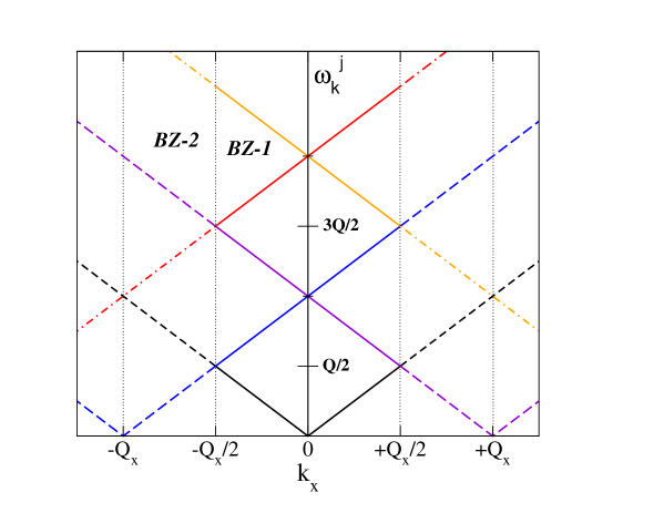
FIG. 3.: Free quasiparticle dispersion relations ($\sigma_{j}\equiv 0$) for massless quarks in a crystal with periodicity in x-direction. The vertical dotted lines indicate the boundaries of the first ($BZ$-1) and second ($BZ$-2) Brillouin Zone (corresponding to $|k_{x}|\leq Q_{x}/2$ and $Q_{x}/2\leq|k_{x}|\leq Q_{x}$, respectively). Plotted are the 5 branches $\omega_{k}^{j}=|k_{x}|$, $|k_{x}\pm Q_{x}|$ and $|k_{x}\pm 2Q_{x}|$ with the full lines characterizing their contributions to $BZ$-1.

Solutions of the gap equations in general support different pairs of $\{\sigma,Q\}$; the combination that minimizes $\Omega(\mu_{q},Q,\sigma)$ is the thermodynamically favored one. Note that the gap equations are not subject to explicit momentum restrictions since off-shell momenta of arbitrary magnitude can in principle contribute.

As a simple example, (27) can be explicitly computed in 1+1 dimensions by recalling that the Fermi surface coincides with the gap, i.e., $\omega_{k_{F}}=\mu_{q}=k_{F}=Q/2$. Specifically, the contribution from the Fermi sea is

$$\Omega_{kin}=\rho\,\epsilon_{F}\,\left(1-\frac{1}{2}\,\left(\sqrt{1+\xi^{2}}+\xi^{2}\,{\rm ln}\,(\xi+\sqrt{1+\xi^{2}})\right)\right)\ ,$$ (28)

with $\xi=\sigma/Q$ and a density $\rho=dk_{F}/\pi$ where $d$ is the overall degeneracy. In MFA, the induced standing wave is $\sigma(x)=2\sigma\,{\rm cos}(Qx)$, and the double counting in the Fermi sea is removed by

$$\Omega_{pot}=\frac{1}{L}\int\,dx\,\frac{\sigma^{2}(x)}{2\lambda}=\frac{\sigma^{2}}{\lambda}\,\,.$$ (29)

The minimum value of $\sigma$ can be obtained in this case analytically by minimizing $\Omega=\Omega_{kin}+\Omega_{pot}$.

III Nonperturbative Forces and Results

For the actual calculations we need to specify the quantum numbers of the pairing channels. To do so we take guidance from low- (or zero-) density phenomenology encoded in effective 4-point interactions. In the particle-hole channel the strongest attraction is in the ’$\sigma$’ channel given by (including exchange terms [4])

$${\cal L}_{mes}^{\sigma}=\frac{\lambda}{8N_{c}^{2}}\ (q\bar{q})^{2}\ ,$$ (30)

whereas in the particle-particle channel it is believed to be the scalar diquark in the color-antitriplet channel (which, in fact, arises from a Fierz-transformation of (30)),

$${\cal L}_{diq}^{\bar{3}}=\frac{\lambda}{8N_{c}^{2}(N_{c}-1)}(q^{T}C\gamma_{5}\tau_{2}\lambda_{A}^{a}q)\ (\bar{q}\tau_{2}\lambda_{A}^{a}\gamma_{5}C\bar{q}^{T})\$$ (31)

($C$: charge conjugation matrix, $\lambda_{A}^{a}$: antisymmetric color matrices, $\tau_{2}$: SU(2)-flavor matrix). For practical use the effective vertices have to be supplemented with ultraviolet cutoffs. In the following we will consider two variants thereof and discuss the pertinent results for the coupled Overhauser/BCS equations.

A NJL Treatment

In a widely used class of Nambu-Jona Lasinio models the ultraviolet behavior of the pointlike vertices is regulated by 3- or 4-momentum multipole formfactors (or even sharp $\Theta$-functions). We here employ a dipole form,

$$F(p)=\left(\frac{\nu\Lambda^{2}}{\nu\Lambda^{2}+p^{2}}\right)^{\nu}$$ (32)

($\nu=2$), for each in- and outgoing quark line with $\Lambda=0.6$ GeV as a typical ’chiral’ scale (variations within such parametrizations do not affect our qualitative conclusions in this section). The coupling constant $\lambda=67$ fm² is calibrated to a constituent quark mass of $M_{q}=0.4$ GeV in vacuum. Note that there is no well-defined way of introducing density dependencies into the interaction. Since at finite $\mu_{q}$ the relevant quark interactions occur at the Fermi surface, a formfactor of type (32) implies the loss of interaction strength with increasing $p_{F}$.

This schematic treatment has been shown to yield robust results for 2-flavor BCS pairing with gaps $\Delta\simeq 0.1$ GeV at quark chemical potentials around 0.5 GeV [1]. Including now the $p$-$h$ pairing as outlined in the previous section we find only rather fragile evidence for the emergence of chiral density waves (at $\mu_{q}=0.4$ GeV): for wave vectors $Q_{x}\leq 0.150$ GeV the rhs of the Overhauser gap equation supports solutions with gaps around $\sim 5$ MeV. The smallness of $Q_{x}$ in fact requires six waves (with $k\pm nQ_{x}$, $n$=1,2,3) to fill all states within the Fermi sphere. Somewhat more robust solutions are obtained when increasing the 4-fermion coupling constant. E.g., with a vacuum constituent quark mass of $M_{q}=0.5$ GeV, which implies $\lambda=73$ fm², the minimum solution emerges for $Q_{x}\simeq 0.2$ GeV and $\sigma\simeq 20$ MeV. However, the gain in the total free energy is very small: $\Omega=-1.2973*10^{-3}$ GeV^-4 as compared to the free Fermi gas value of $\Omega=-1.2969*10^{-3}$ GeV^-4 (to be contrasted with the BCS ground state for which $\Omega_{BCS}(\mu_{q}=0.4~{}{\rm GeV})\simeq-1.375*10^{-3}$ GeV^-4 at a pairing gap of $\Delta\simeq 0.13$ GeV).

We also checked that the incorporation of waves in other spatial directions does not lead to further energy gain.

B Instanton Approach at Finite Chemical Potential

A more microscopic origin of effective 4-fermion interactions is provided within the instanton framework. In the finite-density context it has previously been employed to study the competition between the chiral condensate and two-flavor superconducting quark matter in refs. [14, 4]. Let us briefly recall some elements of the approach. The starting point is the QCD partition function in instanton approximation,

$${\cal Z}_{inst}(\mu_{q})=\frac{1}{N_{+}!~{}N_{-}!}\prod\limits_{I=1}^{N_{+},N_{-}}\int d\Omega_{I}\ n(\rho_{I})\ e^{-S_{int}^{gluon}}\left[det(i\not{\!\!D}-i\mu_{q}\gamma_{4})\right]^{N_{f}}\ ,$$ (33)

where $\Omega_{I}=\{\Theta_{I},\rho_{I},z_{I}\}$ denote the collective coordinates (color, size and position) of the instanton solutions and $n(\rho_{I})$ their individual weight. To extract effective quark interactions one reintroduces quark fields in a way that is compatible with the fermionic determinant of the previous equation [15],

$${\cal Z}_{inst}(\mu_{q})=\int{\cal D}\psi{\cal D}\psi^{\dagger}\exp\left[\int d^{4}x\psi^{\dagger}(i\not\!\partial-i\mu_{q}\gamma_{4})\psi\right]\int\frac{d\lambda_{\pm}}{2\pi}\exp\left[\lambda_{\pm}Y_{\pm}+N_{\pm}\left(\ln\left[\frac{N_{\pm}}{\lambda_{\pm}V_{4}}\right]-1\right)\right]\ ,$$ (34)

and an additional auxiliary integration over $\lambda_{\pm}$ has been introduced to exponentiate the effective (2$N_{f}$)-fermion vertices $Y_{\pm}$. For two flavors the latter are given by

$$\lambda_{\pm}\ Y_{\pm} = \lambda_{\pm}\int\frac{d^{4}k_{1}d^{4}k_{2}d^{4}p_{1}d^{4}p_{2}}{(2\pi)^{16}}\ (2\pi)^{4}\delta^{(4)}(k_{1}+p_{1}-k_{2}-p_{2})\$$ (36)

$$\qquad\qquad\qquad\qquad\times\left[\psi^{\dagger}{\cal F}^{\dagger}(p_{1},-\mu_{q})\gamma_{\pm}\tau_{a}^{-}{\cal F}(k_{1},\mu_{q})\psi\right]\ \left[\psi^{\dagger}{\cal F}^{\dagger}(p_{2},-\mu_{q})\gamma_{\pm}\tau_{a}^{-}{\cal F}(k_{2},\mu_{q})\psi\right]\$$

with $\gamma_{\pm}=(1\pm\gamma_{5})$, flavor matrices $\tau_{\alpha}=(\vec{\tau},i)$ and the instanton formfactors ${\cal F}(p,\mu_{q})=(p+i\mu_{q})^{-}\varphi(p,\mu_{q})^{+}$, which are matrices in Dirac space, adopting the notation of ref. [14], i.e., $x^{\pm}\equiv x_{\mu}\sigma_{\mu}^{\pm}$ with $\sigma_{\mu}^{\pm}\equiv(\pm\vec{\sigma},1)$. Since the fermionic determinant has been approximated by its zero-mode part, the formfactors are entirely determined by the Fourier-transformed quark zero-mode wave functions,

$$\phi_{I,A}(p,\mu_{q}) = \int d^{4}x\ e^{-ip\cdot x}\ \phi_{I,A}(x,\mu_{q})$$ (37)

$$= \varphi(p,\mu_{q})^{\pm}\ \chi_{R,L}$$ (38)

with $\phi(x,\mu_{q})$ satisfying the Dirac equation in the background of an (anti-) instanton,

$$\not\!\!D_{I,A}\ \phi_{I,A}(x)=0\ .$$ (39)

The explicit form of $\varphi_{\mu}(p,\mu_{q})$ can be found in refs. [14, 4].

As before we preselect the potential condensation channels as the scalar-isoscalar $p$-$h$ and $p$-$p$ ones which, after solving the (matrix) Dyson equation, yields the coupled gap equations

$$\Delta = \frac{(-i)\ \lambda}{N_{c}(N_{c}-1)}\int\frac{d^{4}p}{(2\pi)^{4}}\ B(p;\mu_{q})\ F(p;\Delta,\sigma_{j},Q_{j})$$ (40)

$$\left(\sigma_{x}+5~{}\delta\sigma_{x}\right) = \quad\frac{(-i)\ \lambda}{N_{c}}\quad\int\frac{d^{4}p}{(2\pi)^{4}}\ A(p,Q_{x};\mu_{q})\ \ S_{x}(p;\Delta,\sigma_{j},Q_{j})$$ (41)

$$\left(\sigma_{3,x}-10~{}\delta\sigma_{x}\right) = \quad\frac{(-i)\ \lambda}{N_{c}}\quad\int\frac{d^{4}p}{(2\pi)^{4}}\ A(p,Q_{x};\mu_{q})\ \ S_{x}(p;\Delta\equiv 0,\sigma_{3,j},Q_{j})\ .$$ (42)

Here, $\delta\sigma_{j}=\sigma_{j}-\sigma_{3,j}$ denotes the difference in the Overhauser gaps for quarks of color 1,2 ($\sigma_{j}$) or color 3 ($\sigma_{3,j}$) which, respectively, do (eq. (41)) or do not (eq. (42)) participate in the diquark pairing (once $\Delta\neq 0$) [14, 4]. In principle, the wave vectors in the color-1,2 and color-3 channels could also be different when minimizing the free energy. However, the actual solutions for $\sigma_{j}$ and $\sigma_{3,j}$ turn out to be very close to each other even in the presence of large BCS gaps $\Delta$ so that the generically very smooth dependence on the $Q_{j}$ should not cause appreciable deviations between the two color sectors. Under our simplifying assumption that the momentum moduli $|Q_{j}|$ (as well as the associated gap parameters $\sigma_{j}$) of the Overhauser pairing are of equal magnitude the additional $(2n_{w}-2)$ gap equations for the other $p$-$h$ channels are equivalent to (41) and (42). The explicit form of the propagators is given by

$$S_{x}(p,\Delta,\sigma_{j},Q_{j}) = -A(p,Q_{x};\mu_{q})\ \sigma_{x}(p,Q_{x})\ G_{0}(p+Q_{x})\ D(p,\Delta,\sigma_{j},Q_{j})$$ (43)

$$F(p,\Delta,\sigma_{j},Q_{j}) = -B(p;\mu_{q})\ \Delta(p)\ \bar{G}_{0}(p)\ D(p,\Delta,\sigma_{j},Q_{j})$$ (44)

with

$$D(p,\Delta,\sigma_{j},Q_{j})=\bigl{[}\Delta(p)^{2}\bar{G}_{0}(p)-G_{0}^{-1}(p)+\sum\limits_{j}\sigma_{j}(p,Q_{j})^{2}\ G_{0}(p+Q_{j})\bigr{]}^{-1}\ .$$ (45)

The functions $A$ and $B$ represent the (square of the) instanton form factors (normalized to one in vacuum) acting on each fermion line entering/exiting a vertex, and we have introduced the notation $\sigma_{j}(p;Q_{j})\equiv\sigma_{j}A(p;Q_{j})$, $\Delta(p)=\Delta B(p)$. The integration variable $\lambda\equiv\lambda_{\pm}$ plays the role of an effective coupling constant, which, however, is not a priori fixed. Rather, its value is found from minimization of the free energy via a saddle point condition, which reads [14]

$$\frac{N}{V} = \lambda\ \langle Y_{+}+Y_{-}\rangle\ ,$$ (46)

$$= \frac{1}{\lambda}\ [2N_{c}^{2}\sum\limits_{j}{\sigma_{j}}^{2}+4N_{c}(N_{c}-1)\Delta^{2}]\ ,$$ (47)

where $\langle Y_{+}+Y_{-}\rangle$ denotes the ground state expectation value of the interaction vertices with potential condensates. Thus the magnitude of the gaps itself governs the effective coupling to the instantons. In the present treatment the instanton density $N/V$ is assumed to be constant. The final result for the free energy at the minimum then becomes

$$\Omega(\mu_{q})=-\frac{\ln{\cal Z}}{V}=\Omega_{kin}(\mu_{q})+\frac{N}{V}\ln\left[\frac{\lambda}{(N/V)}\right]\ ,$$ (48)

indicating that the potential (second) term favors small values for $\lambda$, whereas the kinetic (first) term exhibits the usual decrease with increasing values for the gaps/condensates (and thus for $\lambda$). We should also point out that $\Omega(\mu_{q})$ is only determined up to an overall constant which is associated with the nonperturbative vacuum energy of about $-0.5$ GeV/fm³ (or, equivalently, bag pressure $P$$>$0). This term is encoded in the scale dependence of the argument in the logarithm (note that $\lambda$ and $N/V$ have different dimensions), which we have not assessed here since it is not relevant for our analysis (this will be the origin of positive values for $\Omega(\mu_{q})$ encountered below).

Before we come to the numerical solutions of the gap equations let us recall the specific density dependence of the instanton formfactors, cf. fig. 4. At fixed energy (upper panel) the strength of the interaction is clearly concentrated at the Fermi surface: the falloff with three-mometum sets in only above $p\simeq p_{F}$. On the other hand, as a function of (Euclidean) energy the strength is reduced starting from $p_{4}=0$ (see lower panel). These features reflect that the instanton zero-modes, which mediate the interaction, operate across the Fermi surface, i.e., at zero energy but at 3-momenta equal to the Fermi momentum. This behavior is quite distinct from the schematic (density-independent) NJL forces employed in the previous section. Already at this point one can anticipate the Overhauser pairing to be more competitive than in the NJL treatment.

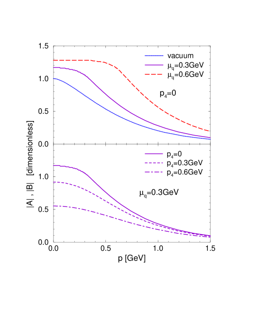
FIG. 4.: In-medium instanton form factors as a function of three-momentum. Upper panel: at fixed energy $p_{4}=0$ for chemical potetnials $\mu_{q}=0$, 0.3 GeV, 0.6 GeV; lower panel: for fixed $\mu_{q}=0.3$ GeV and various energies.

For the evaluation of the kinetic part of the free energy as given in eq. (27) a complication arises from the fact that the the instanton formfactors are defined in Euclidean space. We therefore approximated the gaps entering into the integral for $\Omega_{kin}$ by their zero-energy values retaining the 3-momentum dependence, i.e., $\Delta(p)\simeq\Delta(\vec{p})=\Delta B(p_{4}=0,\vec{p})$, and equivalently for $\sigma$. It turns out that this approximation is consistent in the sense that the resulting extrema in $\Omega$ are in line with the solutions of the gap equations (which are solved in Euclidean space with the full 4-momentum dependence of the formfactors). Other choices for fixing $p_{4}$ do not comply with this criterium.

If not otherwise stated, the subsequent calculations have been performed for a total instanton density of $N/V=1$ fm^-4 which in vacuum translates into a constituent quark mass of $M_{q}=0.34$ GeV. The search for simultaneous solutions to the gap equations (40), (41) and (42) together with the selfconsistency condition on the coupling, eq. (47), is illustrated in fig. 5. The upper two curves represent the values for $\sigma$ and $\sigma_{3}$ that simulatneuosly solve the two Overhauser gap eqs. (41) and (42) at given BCS gap $\Delta$ (plotted on the abscissa). The lower curve indicates the values for $\sigma$ that solve the BCS gap eq. (40) for given $\Delta$ (using the value for $\sigma_{3}$ from the upper curve to fix the coupling $\lambda$). Thus a coexistence state of Overhauser and BCS pairing would be signalled by the crossing of the two lower lines. As mentioned above no such state is found; the only physical solutions correspond to the crossing points of the upper (full or dashed) curve with the $y$-axis (Overhauser state with $\Delta=0$, $\sigma=\sigma_{3}$ finite) and of the lower (dashed-dotted) curve with the $x$-axis (BCS state with $\sigma=\sigma_{3}=0$ and $\Delta=0.225$ GeV; the discrepancy of about 15% (less at higher $\mu_{q}$) with refs. [14, 4] reflects the accuracy when neglecting antiparticle states).

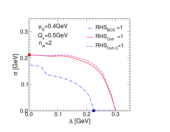
FIG. 5.: Solutions of the coupled Overhauser and BCS equations with 2 waves at $Q_{x}=\pm 0.5$ GeV. The full and dashed lines indicate, respectively, the values for $\sigma_{x}(\Delta)$ and $\sigma_{3,x}(\Delta)$ which simultaneously solve the two Overhauser gap equations (41) and (42) for given $\Delta$. The dashed-dotted line corresponds to the points $\sigma_{x},\Delta$ that solve the BCS gap equation (40). A nontrivial simultaneous solution to all 3 gap equations would be signalled by a crossing of the full and dashed-dotted curves. The two independent pure BCS and Overhauser solutions are marked by the squares on the $x$- and $y$-axis, respectively.

The question then is which one is thermodynamically favored. The BCS solution is unique ($\Delta=0.225$ GeV) and gives a total free energy of $\Omega_{BCS}(\mu_{q}=0.4~{}{\rm GeV})=2.3*10^{-3}$ GeV⁴ (up to a constant which is not relevant here, as discussed above).

The situation is more involved for the Overhauser configurations. Let us start with the ’canonical’ case where the momentum vector of the chiral density waves is fixed at twice the Fermi momentum, $Q=2p_{F}$. In fig. 6 the resulting minimized free energy (corresponding to solutions of eq. (41)) is displayed as function of the number of included waves. The Overhauser solutions are not far above the BCS groundstate, with a slight energy gain for an increased number of waves.

However, one can further economize the energy of the Overhauser state by exploiting the freedom associated with the wave vector $Q$ (or, equivalently, the periodicity of the lattice). For $Q>2p_{F}$ the free energy rapidly increases. On the other hand, for $Q<2p_{F}$ more favorable configurations are found. To correctly assess them one has to include the waves in pairs $|k\pm Q_{j}|$ of standing waves (i.e., $n_{w}=2,4,6,\dots$) to ensure that the occupied states in the Fermi sea are saturated within the first Brillouin Zone (cf. fig. 3). The lowest-lying state we could find at $\mu_{q}=0.4$ GeV occurs for one standing wave with $Q_{min}\simeq 0.5$ GeV and $\sigma\simeq 0.21$ GeV with a free energy $\Omega\simeq 2.3*10^{-3}$ GeV⁴, practically degenerate with the BCS solution. In solid state physics the breaking of translational invariance in one spatial direction is typically associated with ’liquid crystals’, i.e., 2-dimensional layers of (uniform) liquid separated by periodic spacings of $a=2\pi/Q$. In our case, $a\simeq 2.5$ fm. The minimum in the wave vector is in fact rather shallow, as seen from the explicit momentum dependence of the free energy displayed in fig. 7.

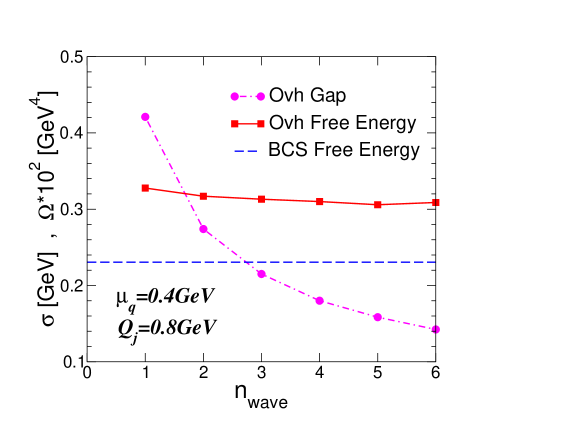
FIG. 6.: Dependence of the free energy (upper full line) and associated $p$-$h$ pairing gap (dashed-dotted) on the number of included waves (’patches’) with fixed 3-momentum modulus $|\vec{Q}_{j}|=0.8$ GeV for solutions of eqs. (41) and (47); the full line marks the value of the BCS ground state free energy that solves eqs. (40) and (47). The results are for $\mu_{q}=0.4$ GeV and $N/V=1$ fm^-4.

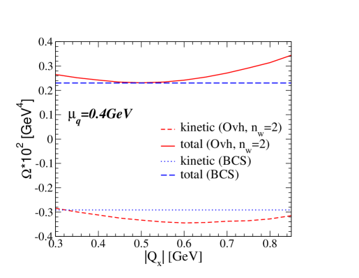
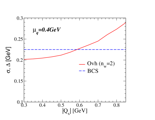
FIG. 7.: Left panel: wave-vector dependence of the Overhauser free energy for one standing wave (full line: $\Omega_{tot}^{Ovh}$, short-dashed line: $\Omega_{kin}^{Ovh}$) in comparison to the BCS solution (long-dashed line: $\Omega_{tot}^{BCS}$, dotted line: $\Omega_{kin}^{BCS}$) at $\mu_{q}=0.4$GeV (we note again that the absolute values of the total free energies are only determined up to an overall (negative) constant (related to the ’bag presssure’) which drops out in the relative comparison of the solutions); right panel: wave-vector dependence of the Overhauser pairing gap (full line) compared to the BCS gap (long-dashed line).

Finally we confront in fig. 8 the density dependence of the free energies (upper panel) and pairing gaps (lower panel) in the minimum of the BCS and $n_{w}$=2,6 Overhauser states. Again we see that over the applicable $\mu_{q}$-range the solutions are close in energy, with (almost) degenerate minima for the $n_{w}$=2-’liquid crystal’ and the BCS ground state at the lower densities of $\rho_{B}\simeq 4\rho_{0}$. Towards higher densities, where the gaps and thus the strength of the effective instanton interactions decrease, the BCS solution becomes relatively more favorable. This confirms once more that in the 3+1 dimensions the Overhauser pairing can only compete for sufficiently strong coupling. We should also note that for both the $n_{w}$=2- and $n_{w}$=6-case as displayed the optimal momentum vector of the pertinent standing waves stays at approximate values of $Q_{j}\simeq 5p_{F}/4$ and $5p_{F}/3$, respectively.

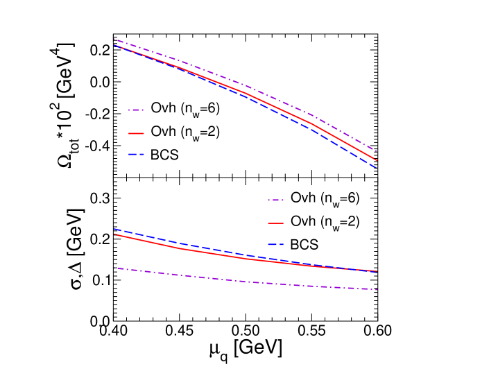
FIG. 8.: Chemical potential dependence of the total free energies (upper panel) and pairing gaps (lower panel) for the BCS (long-dashed lines) and Overhauser (solid and dashed-dotted lines) solutions.

IV Concluding Remarks

Employing a standard Nambu-Gorkov (matrix) propagator approach we have performed an analysis of competing instabtilities in the particle-particle and particle-hole channel for three-color, two-flavor QCD at moderate quark densities. As an essential ingredient we used nonperturbative forces (strong coupling) and preselected the potential condensation channels with guidance from low-energy hadron phenomenology, i.e., both the diquark as well as the quark-hole pairing were evaluated in their scalar-isoscalar channels. The corresponding coupled gap equations do not seem do support simultaneous nontrivial solutions. Needless to say that our calculations might be further improved by including higher standing waves through a larger class of crystalline symmetries (polyhedron structures). Also, our mean-field approximation may be extended to account for higher intra-band mixings when $2\mu_{q}>Q$.

This not withstanding, an important outcome of our calculation is that the individual (separate) solutions for the BCS and Overhauser ground states are quite close in energy, indicating the importance of particle-hole instabilities when using interaction strengths as typical for low-energy hadronic binding. This becomes particularly evident when comparing schematic NJL interactions with microscopic instanton forces: whereas the former are reduced in magnitude with increasing density (entailing a relative suppression of the Overhauser pairing), the density-dependent instanton form factors essentially preserve their strength at the Fermi surface rendering the Overhauser pairing competitive. Indeed, with a somewhat larger instanton-density of $N/V=1.4$ fm^-4, corresponding to a vacuum constituent quark mass of $M_{q}=0.41$ GeV, the Overhauser solution reaches below the BCS one. On the other hand, if we were to minimally account for strange quarks, the instanton interaction (being a 6-quark vertex) in the $ud$ sector would lose about 60% of its strength due to the reduced strange-quark mass ($m_{s}\simeq$ 0.15 GeV as opposed to $M_{s}\simeq 0.45$ GeV in vacuum) in closing-off the strange quark line. Some of this loss might be recovered once strange quarks themselves participate in the Overhauser pairing. Our findings are to be contrasted with earlier calculations based on perturbative OGE at high densities where an extremely large number of colors was required for the Overhauser pairing (i.e., a chiral density wave) to overcome the BCS instability.

Finally, a remark about the relevance of our results for neutron stars is in order. Here, quark matter is believed to reside mostly in a mixed phase, with significant charge separation between quark and nuclear components. The quark core, however, also exhibits charge asymmetry due to the finite strange quark mass. Consequently, quark matter should have appreciably different up- and down-quark chemical potentials, which suppresses the flavor-singlet diquark ($ud$) pairing [16]. On the other hand, such a suppression does not apply to the (flavor-singlet) particle-hole channels of type $uu^{-1}$, $dd^{-1}$, which suggests that isopin asymmetric quark matter provides additional favor to the chiral crystal.

REFERENCES

- [1] M. Alford, K. Rajagopal and F. Wilczek, Phys. Lett. B422, 247 (1998).
- [2] R. Rapp, T. Schäfer, E. V. Shuryak and M. Velkovsky, Phys. Rev. Lett. 81, 53 (1998).
- [3] M. Alford, K. Rajagopal and F. Wilczek, Nucl. Phys. B537, 443 (1999).
- [4] R. Rapp, T. Schäfer, E.V. Shuryak and M. Velkovsky, Ann. Phys. 280, 35 (2000).
- [5] R.E. Peierls, Quantum Theory of Solids, Oxford University Press (London, 1955), p.108.
- [6] A.W. Overhauser, Phys. Rev. 128, 1437 (1962); Adv. Phys. 27, 343 (1978).
- [7] G. Grüner, Rev. Mod. Phys. 66, 1 (1994).
- [8] D.V. Deryagin, D.Y. Grigoriev and V.A. Rubakov, Int. J. Mod. Phys. A7, 659 (1992).
- [9] E. Shuster and D.T. Son, hep-ph/9905448.
- [10] B.-Y. Park, M. Rho, A. Wirzba and I. Zahed, hep-ph/9910347.
- [11] A.B. Migdal, E.E. Saperstein, M.A. Troitsky and D.N. Voskresensky, Phys. Rep. 192, 179 (1990).
- [12] L. Castillejo, P.S.J. Jones, A.D. Jackson, J.J.M. Verbaarschot and A. Jackson, Nucl.Phys. A501, 801 (1989).
- [13] R.D. Mattuck and B. Johansson, Adv. Phys. 17, 509 (1968).
- [14] G.W. Carter and D. Diakonov, Phys. Rev. D60, 106004 (1999).
- [15] D. Diakonov and V.Yu. Petrov, preprint LNPI-1153 (1986), publ. in Hadron matter under extreme condtions, Kiev (1986) 192; see also D. Diakonov, hep-ph/9602375.
- [16] P.F. Bedaque, hep-ph/9910247.