QCD IN A FINITE VOLUME INLO-PUB-08/00

Abstract

We will review our understanding of non-abelian gauge theories in finite physical volumes. It allows one in a reliable way to trace some of the non-perturbative dynamics. The role of gauge fixing ambiguities related to large field fluctuations is an important lesson that can be learned. The hamiltonian formalism is the main tool, partly because semiclassical techniques are simply inadequate once the coupling becomes strong. Using periodic boundary conditions, continuum results can be compared to those on the lattice. Results in a spherical finite volume will be discussed as well.

1 Introduction

We have decided to take this opportunity of contributing to a handbook of QCD, in honor of Boris Lazarevich Ioffe, to bring together results and methods that were developed in solving for the low-lying spectrum in a finite volume. The emphasis will be on the dynamical aspects of the classically scale invariant theory for non-abelian gauge theories in 3+1 dimensions.[1] The challenge is to understand how the mass gap is generated. Due to the need for regularization, at the quantum level breaking the scale invariance, a running coupling appears. The difficulty lies in the fact that this coupling increases at low-energies and long-distance scales, beyond the point where one has control over the field fluctuations, which become so large that they probe the essential non-linearities of the theory. A finite volume explicitly breaks the scale invariance. However, it does so in a rather mild way. Classically one can use the scale transformation to go from one physical volume to another, and only the running of the coupling constant prevents us from taking the infinite volume limit. As the longest distance scale, i.e. the lowest energy scale, is set by the volume, one can keep in check the growth of the running coupling constant.

We will describe the results mainly in the context of a hamiltonian picture [2] with wave functionals on configuration space. Although rather cumbersome from a perturbative point of view, where the covariant path integral approach of Feynman is vastly superior, it provides more intuition on how to deal with non-perturbative contributions in situations where semi-classical techniques can no longer be used, like for observables that do not vanish in perturbation theory. The high energy modes can be well-approximated by a harmonic oscillator contribution to the wave functional. In the direction of these field modes the potential energy rises steeply. Their contribution, including regulating the ultraviolet behavior, is treated perturbatively, giving in particular rise to the running of the coupling. The finite volume allows us to have a well-defined mode expansion. Due to the classical scale invariance, the hamiltonian can be formulated in terms of dimensionless fields. This can be extended to the quantum theory, as Ward identities allow for a field definition without anomalous scaling. Apart from the overall scaling dimension of the hamiltonian, only the running coupling introduces a non-trivial volume dependence.

Due to the non-abelian nature of the theory the physical configuration space, formed by the set of gauge orbits $\mbox{$\cal A$}/\mbox{$\cal G$}$ ($\cal A$ is the collection of connections, $\cal G$ the group of local gauge transformations) is non-trivial.[3] Most frequently, coordinates of this orbit space are chosen by picking a representative gauge field on the orbit in a smooth and preferably unique way. Linear gauge conditions like the Landau or Coulomb gauge suffer from what is known as Gribov ambiguities.[4] The region of field space that contains no further gauge copies is called a fundamental domain for non-abelian gauge theories.[5]

Having arranged the low-energy field modes (and all those modes not affected by the cutoff) to be scale invariant, the spreading of the wave functional is completely caused by an increasing coupling. This is what leads to non-perturbative effects. Asymptotic freedom on the other hand guarantees that in small volumes the running coupling is small and it thus keeps the wave functional localized near the classical vacuum manifold. In a periodic geometry, this perturbative analysis was pioneered by Bjorken [6] and further developed by Lüscher [7]. The essential ingredient we have added to address non-perturbative effects is boundary conditions in field space, at the boundary of the fundamental domain, with gauge invariance implemented properly at all stages.

The non-perturbative features due to spreading of the wave functional can be followed out to a physical volume of about one cubic fermi (setting the scale by the string tension or lowest glueball state). This is, on the basis of a comparison with lattice Monte Carlo data, the point where in the pure gauge theory the confining string is being formed, with no significant finite volume dependence beyond this volume. What has become clear is that the transition from the finite to the infinite volume is driven by field fluctuations that cross the barrier which is associated with tunneling between different classical vacua. This is natural, since this barrier (the finite volume sphaleron), will be the direction beyond which the wave functional can first spread most significantly, as it provides the lowest mountain pass in the energy landscape.

In Sec. 2 we describe the process of complete gauge fixing, and the fact that the boundary of the fundamental domain, unlike its interior, has gauge copies that implement the non-trivial topology of configuration space. This is applied in Sec. 3 to formulating non-abelian gauge theories on a torus, both for SU(2) and in Sec. 3.1 for SU(3). The influence of massless quarks on the small volume vacuum structure is discussed in Sec. 3.2, whereas Sec. 3.3 gives a short review of the non-perturbative evaluation of the running renormalized coupling, making explicit use of the finite volume geometry.[8] In Sec. 3.4 we consider the case of twisted boundary conditions,[9] and in Sec. 3.5 we discuss supersymmetric Yang-Mills theory in a finite volume in the light of some recent developments concerning the Witten index.[10] Sec. 4 outlines what is known about instantons on the torus, reviewing the Nahm transformation [11] in Sec. 4.1. Sec. 5 analyzes the situation for a spherical geometry, particularly well adapted to study the role of instantons in the low-lying glueball spectrum. Finally, we shall consider the behavior in large finite volumes. We discuss how the previous results fit together and what this implies. In Secs. 6.1 and 6.2 we review the volume dependence whenever the polarization clouds are well-contained in the finite volume.[12] In Sec. 6.3 we briefly mention the situation in the absence of a mass gap, particularly relevant for QCD with its light up and down quarks, for which chiral perturbation theory applies.[13] We conclude with a review of ’t Hooft’s electric-magnetic duality on the torus [9] in Sec. 6.4.

2 Complete Gauge Fixing

An (almost) unique representative of the gauge orbit is found by minimizing the $L^{2}$ norm of the vector potential along the gauge orbit [5, 14]

$$G_{A}(h)\equiv\left\|[h]A\right\|^{2}=-\int_{M}\mbox{\,tr\,}\left(\left(h^{-1}({\bf x})A_{i}({\bf x})h({\bf x})+h^{-1}({\bf x})\partial_{i}h({\bf x})\right)^{2}\right),$$ (1)

where the vector potential is taken anti-hermitian, the integral over the finite spatial volume $M$ is with the appropriate canonical volume form and $h({\bf x})$ is a Lie-group element, with $[h]A$ a short-hand notation for the associated gauge transformation. Note that in these conventions the field strength is given by

$$F_{\mu\nu}({\bf x},t)=\partial_{\mu}A_{\nu}({\bf x},t)-\partial_{\nu}A_{\mu}({\bf x},t)+[A_{\mu}({\bf x},t),A_{\nu}({\bf x},t)]$$ (2)

and the action by

$$L(t)={\scriptstyle{{1\over 2}}}\int_{M}g^{-2}\mbox{\,tr\,}(F_{\mu\nu}^{\,2}({\bf x},t)).$$ (3)

Expanding around the minimum of Eq. (1), writing $h({\bf x})=\exp(X({\bf x}))$ ($X({\bf x})$ is, like the gauge field $A_{i}({\bf x})$, an element of the Lie-algebra) one easily finds

$$\left\|\,[h]A\right\|^{2} = \left\|A\right\|^{2}+2\int_{M}\mbox{\,tr\,}(X\partial_{i}A_{i})+\int_{M}\mbox{\,tr\,}(X^{\dagger}FP(A)X)$$

$$\hskip-36.98866pt+\frac{1}{3}\int_{M}\mbox{\,tr\,}\left(X\left[[A_{i},X],\partial_{i}X\right]\right)+\frac{1}{12}\int_{M}\mbox{\,tr\,}\left([\mbox{$\cal D$}_{i}X,X][\partial_{i}X,X]\right)+\mbox{$\cal O$}\left(X^{5}\right),$$

where $FP(A)$ is the Faddeev-Popov operator $({\rm ad}(A)X\equiv[A,X])$

$$FP(A)=-\partial_{i}\mbox{$\cal D$}_{i}(A)\equiv-\partial_{i}(\partial_{i}+{\rm ad}(A_{i})).$$ (5)

At a local minimum the vector potential is therefore transverse, $\partial_{i}A_{i}=0$, and $FP(A)$ is a positive operator. The set of all these vector potentials is by definition the Gribov region $\Omega$. Using the fact that $FP(A)$ is linear in $A$, $\Omega$ is seen to be a convex subspace of the set of transverse connections $\Gamma$. Its boundary $\partial\Omega$ is called the Gribov horizon. At the Gribov horizon, the lowest non-trivial eigenvalue of the Faddeev-Popov operator vanishes, and points on $\partial\Omega$ are associated with coordinate singularities. Any point on $\partial\Omega$ can be seen to have a finite distance to the origin of field space and in some cases even uniform bounds can be derived.[15, 16]

The Gribov region is the set of local minima of the norm functional, Eq. (1), and needs to be further restricted to the absolute minima to form a fundamental domain, [5] which will be denoted by $\Lambda$. The fundamental domain is clearly contained within the Gribov region. To show that also $\Lambda$ is convex, note that

$$\left\|\,[h]A\right\|^{2}-\left\|A\right\|^{2}=\int\mbox{\,tr\,}\left(A_{i}^{2}\right)-\int\mbox{\,tr\,}\left(\left(h^{-1}A_{i}h+h^{-1}\partial_{i}h\right)^{2}\right)$$ (6)

$$\quad=\int\mbox{\,tr\,}\left(h^{\dagger}FP_{f}(A)\,h\right)\equiv\left\langle h,FP_{f}(A)\,h\right\rangle,\quad FP_{f}(A)\equiv-\partial_{i}D_{i}(A),$$

where $FP_{f}(A)$ acts on the fundamental representation and is similar to the Faddeev-Popov operator. Both $FP(A)$ and $FP_{f}(A)$ are hermitian operators when $A$ is a critical points of the norm functional, i.e. for $A$ transverse. We can define $\Lambda$ in terms of the absolute minima over $h\in\mbox{$\cal G$}$ of $\left\langle h,FP_{f}(A)\,h\right\rangle$

$$\Lambda=\{A\in\Gamma|\min_{h\in\mbox{$\cal G$}}\left\langle h,FP_{f}(A)\,h\right\rangle=0\}.$$ (7)

Using that $FP_{f}(A)$ is linear in $A$, the convexity of $\Lambda$ is automatic: A line connecting two points in $\Lambda$ lies within $\Lambda$.

If we would not specify anything further, as a convex space is contractible, the fundamental region could never reproduce the non-trivial topology of the configuration space. This means that $\Lambda$ should have a boundary.[17] Indeed, as $\Lambda$ is contained in $\Omega$, this means $\Lambda$ is also bounded in each direction. Clearly $A=0$ is in the interior of $\Lambda$, which allows us to consider a ray extending out from the origin into a given direction, where it will have to cross the boundary of $\Lambda$ and $\Omega$. For any point along this ray in $\Lambda$, the norm functional is at its absolute minimum as a function of the gauge orbit. However, for points in $\Omega$ that are not also in $\Lambda$, the norm functional is necessarily at a relative minimum. The absolute minimum for this orbit is an element of $\Lambda$, but in general not along the ray. Continuity therefore tells us that at some point along the ray, this absolute minimum has to pass the local minimum. At the point they are exactly degenerate, there are two gauge equivalent vector potentials with the same norm, both at the absolute minimum. As in the interior the norm functional has a unique minimum, again by continuity, these two degenerate configurations have to both lie on the boundary of $\Lambda$.

When $L$ denotes the linear size of $M$, we may express the gauge fields in the dimensionless combination of $LA$ (in our conventions the fields have no anomalous scale dependence), and the shape and geometry of the Gribov and fundamental regions are scale independent. We should note that the norm functional is degenerate along the constant gauge transformations and indeed the Coulomb gauge does not fix these gauge degrees of freedom. We simply demand that the wave functional is in the singlet representation under the constant gauge transformations and we have $\Lambda/G=\mbox{$\cal A$}/\mbox{$\cal G$}$. Here $\Lambda$ is assumed to include the non-trivial boundary identifications that restore the non-trivial topology of $\mbox{$\cal A$}/\mbox{$\cal G$}$.

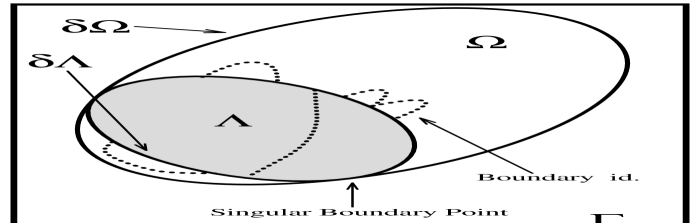
Figure 1: Sketch of the fundamental (shaded) and Gribov regions. The dotted lines indicate the boundary identifications.

If a degeneracy at the boundary is continuous, other than by constant gauge transformations, one necessarily has at least one non-trivial zero eigenvalue for $FP(A)$ and the Gribov horizon will touch the boundary of the fundamental domain at these so-called singular boundary points. We sketch the general situation in Fig. 1. In principle, by choosing a different gauge fixing in the neighborhood of these points one could resolve the singularity. If singular boundary points would not exist, all that would have been required is to complement the hamiltonian in the Coulomb gauge with the appropriate boundary conditions in field space. Since the boundary identifications are by gauge transformations the boundary condition on the wave functionals is simply that they are identical under the boundary identifications, possibly up to a phase in case the gauge transformation is homotopically non-trivial.

Unfortunately, one can argue that singular boundary points are to be expected.[17] Generically, at singular boundary points the norm functional undergoes a bifurcation moving from inside to outside the fundamental (and Gribov) region. The absolute minimum turns into a saddle point and two local minima appear, as indicated in Fig. 2. These are necessarily gauge copies of each other. The gauge transformation is homotopically trivial as it reduces to the identity at the bifurcation point, evolving continuously from there on.

Figure 2: Sketch of a singular boundary point due to a bifurcation of the norm functional. It can be used to show that there are homotopically trivial gauge copies inside the Gribov horizon (H).

Also Gribov’s original arguments for the existence of gauge copies [4] (showing that points just outside the horizon are gauge copies of points just inside) can be easily understood from the perspective of bifurcations in the norm functional. It describes the generic case where the zero-mode of the Faddeev-Popov operator arises because of the coalescence of a local minimum with a saddle point with only one unstable direction. At the Gribov horizon the norm functional locally behaves in that case as $X^{3}$, with $X$ the relevant zero eigenfunction of the Faddeev-Popov operator. The situation sketched in Fig. 2 corresponds to the case where the leading behavior is like $X^{4}$.

The necessity to restrict to the fundamental domain, a subset of the transverse gauge fields, introduces a non-local procedure in configuration space. This cannot be avoided since it reflects the non-trivial topology of this space. We stress again that its topology and geometry is scale independent. Homotopical non-trivial gauge transformations are in one to one correspondence with non-contractible loops in configuration space, which give rise to conserved quantum numbers. The quantum numbers are like the Bloch momenta in a periodic potential and label representations of the homotopy group of gauge transformations. On the fundamental domain the non-contractible loops arise through identifications of boundary points. Although slightly more hidden, the fundamental domain will therefore contain all the information relevant for the topological quantum numbers. Sufficient knowledge of the boundary identifications will allow for an efficient and natural projection on the various superselection sectors. Typically we integrate out the high-energy modes, being left with the low-energy modes whose dynamics is determined by an effective hamiltonian defined on the fundamental domain (restricted to these low-energy modes). In this it is assumed that the contributions of the high-energy modes can be dealt with perturbatively, generating the running coupling and the effective interactions of the low-energy modes. We will in detail discuss the results for finite volumes with a torus and sphere geometry.

3 Gauge Fields on the three-Torus

Probably the most simple example to illustrate the relevance of the fundamental domain is provided by gauge fields on the torus in the abelian zero-momentum sector. Let us first take $G$=SU(2) and $A_{j}=i{C_{j}\over 2L}\tau_{3}$ ($L$ is the size of the torus, $\tau_{j}$ are the Pauli matrices). These modes are dynamically motivated as they form the set of gauge fields on which the classical potential vanishes. It is called the vacuum valley (sometimes also referred to as toron valley) and one can attempt to perform a Born-Oppenheimer-like approximation for deriving an effective hamiltonian in terms of these “slow” degrees of freedom. To find the Gribov horizon, one easily verifies that the part of the spectrum for $FP(A)$ that depends on ${\bf C}$, is given by $\lambda^{gh}_{{\bf n}}({\bf C})=2\pi{\bf n}\cdot(2\pi{\bf n}\pm{\bf C})/L^{2}$, with ${\bf n}\neq{\bf 0}$ an integer vector. The lowest eigenvalue vanishes if $C_{j}=\pm 2\pi$. The Gribov region is therefore a cube with sides of length $4\pi$, centered at the origin, specified by $|C_{j}|\leq 2\pi$ for all $j$, see Fig. 3.

The gauge transformation $h_{(j)}=\exp(\pi ix_{j}\tau_{3}/L)$ maps $C_{j}$ to $C_{j}+2\pi$, leaving the other components $C_{i\neq j}$ untouched. As $h_{(j)}$ is anti-periodic it is homotopically non-trivial (they are ’t Hooft’s twisted gauge transformations.[9]) We thus see explicitly that gauge copies occur inside $\Omega$, but furthermore the naive vacuum $A=0$ has (many) gauge copies under these shifts of $2\pi$ that lie on the Gribov horizon. It can actually be shown in the Coulomb gauge that for any three-manifold, any Gribov copy by a homotopically non-trivial gauge transformation of $A=0$ will have a non-trivial zero eigenvalue for the Faddeev-Popov operator.[17] Taking the symmetry under homotopically non-trivial gauge transformations properly into account is crucial for describing the non-perturbative dynamics and one sees that the singularity of the hamiltonian at Gribov copies of $A=0$, where the wave functionals are in a sense maximal, could form a severe obstacle in obtaining reliable results.

To find the boundary of the fundamental domain we note that the gauge copies ${\bf C}=(\pi,C_{2},C_{3})$ and ${\bf C}=(-\pi,C_{2},C_{3})$ have equal norm. The boundary of the fundamental domain, restricted to the vacuum valley formed by the abelian zero-momentum gauge fields therefore occurs where $|C_{j}|=\pi$, well inside the Gribov region, see Fig. 3. The boundary identifications are by the homotopically non-trivial gauge transformations $h_{(j)}$. The fundamental domain, described by $|C_{j}|\leq\pi$ with all boundary points regular, has the topology of a torus. To be more precise, as the remnant of the constant gauge transformations (the Weyl group) changes ${\bf C}$ to $-{\bf C}$, the fundamental domain $\Lambda/G$ restricted to the abelian constant modes is the orbifold $T^{3}/Z_{2}$. As we will see, the orbifold singularities are associated with problems in using the harmonic approximation in perturbation theory for modes orthogonal to those of vacuum valley.

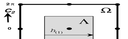
Figure 3: A two dimensional slice of the vacuum valley along the $(C_{1},C_{2})$ plane. The fat square give the Gribov horizon, the grey square is the fundamental domain. The dots at the Gribov horizon are Gribov copies of the origin.

Formulating the hamiltonian on $\Lambda$, with the boundary identifications implied by the gauge transformations $h_{(j)}$, avoids the singularities at the Gribov copies of $A=0$. “Bloch momenta” associated with the $2\pi$ shift, implemented by the non-trivial homotopy of $h_{(j)}$, label ‘t Hooft’s electric flux quantum numbers [9] $\Psi(C_{j}=-\pi)=\exp(\pi ie_{j})\Psi(C_{j}=\pi)$. Note that the phase factor is not arbitrary, but $\pm 1$. This is because $h^{2}_{(j)}$ is homotopically trivial. In other words, the homotopy group of these anti-periodic gauge transformations is $Z_{2}^{3}$. Considering a slice of $\Lambda$ can obscure some of the topological features. A loop that winds around the slice twice is contractible in $\Lambda$ as soon as it is allowed to leave the slice. Indeed including the lowest modes transverse to this slice will make the $Z_{2}$ nature of the relevant homotopy group evident.[18] It should be mentioned that for the torus in the presence of fields in the fundamental representation (quarks), only periodic gauge transformations are allowed.[19] This will be discussed in Sec. 3.2.

In weak coupling Lüscher showed unambiguously that the wave functionals are localized around $A=0$, that they are normalizable and that the spectrum is discrete.[6, 7] In this limit the spectrum is insensitive to the boundary identifications (giving rise to a degeneracy in the topological quantum numbers). This is manifested by a vanishing electric flux energy, defined by the difference in energy of a state with $|{\bf e}|=1$ and the vacuum state with ${\bf e}={\bf 0}$. Although there is no classical potential barrier to achieve this suppression, it comes about by a quantum induced barrier, in strength down by two powers of the coupling constant.

$$V({\bf C})=2L^{-1}\sum_{{\bf p}\in{\rm Z\!\!Z}^{3}}(|2\pi{\bf p}+{\bf C}|-|2\pi{\bf p}|)=\frac{4}{L\pi^{3}}\sum_{{\bf n}\neq{\bf 0}}\frac{\sin^{2}({\scriptstyle{{1\over 2}}}{\bf n}\cdot{\bf C})}{({\bf n}\cdot{\bf n})^{2}}.$$ (8)

The second identity is obtained by Poisson resummation,[7] and the periodicity reflects the gauge symmetry discussed above. This quantum induced barrier leads to a suppression [20] with a factor $\exp(-S/g)$ instead of the usual factor of $\exp(-8\pi^{2}/g^{2})$ for instantons.[21, 22] The associated tunneling configuration was called a pinchon.[20] At stronger coupling the wave functional spreads out over the vacuum valley and drastically changes the spectrum.[23] At this point the energy of electric flux suddenly switches on.

Integrating out the non-zero momentum modes, for which Bloch degenerate perturbation theory [24] provides a rigorous framework,[7] one finds an effective hamiltonian. Near $A=0$, due to the quartic nature of the potential energy $V(A)=-{\scriptstyle{{1\over 2}}}\int d^{3}x\mbox{\,tr\,}(F^{\,}_{ij})$ for the zero-momentum modes (the derivatives vanish, such that the field strength is quadratic in the field), there is no separation in time scales between the abelian and non-abelian modes. Away from $A=0$ one could further reduce the dynamics to one along the vacuum valley, but near the origin the adiabatic approximation breaks down. This gives rise to a conic singularity, $V({\bf C})=2|{\bf C}|/L+\mbox{$\cal O$}\left(C^{2}\right)$, due to fluctuations of the non-abelian zero-momentum modes (contributing the ${\bf p}={\bf 0}$ term in Eq. (8)).

The effective hamiltonian is expressed in terms of the coordinates $c_{j}^{a}$, where $i=\{1,2,3\}$ is the spatial index ($c_{0}^{a}=0$) and $a=\{1,2,3\}$ the SU(2)-color index. It will be convenient to introduce $f_{jk}^{a}\equiv-\epsilon_{abd}c_{j}^{b}c_{k}^{d}$ and $r_{j}\equiv\sqrt{\sum_{a}c_{j}^{a}c_{j}^{a}}$. The latter are gauge-invariant “radial” coordinates, that will play a crucial role in specifying the boundary conditions. The zero-momentum gauge field and field strength read $A_{j}({\bf x})=ic_{j}^{a}\frac{\tau_{a}}{2L}$ and $F_{jk}=if_{jk}^{a}\frac{\tau_{a}}{2L^{2}}$. For dimensional reasons the effective hamiltonian is proportional to $1/L$. It will furthermore depend on $L$ through the renormalized coupling constant ($g(L)$) at the scale $\mu=1/L$. To one loop order (for small $L$) $g^{2}(L)=12\pi^{2}/[-11\ln(\Lambda_{MS}L)]$. One expresses the masses and the size of the finite volume in dimensionless quantities, like mass-ratios and the parameter $z=mL$. In this way, the explicit dependence of $g$ on $L$ is irrelevant. This is also the preferred way of comparing results obtained within different regularization schemes (e.g. dimensional and lattice regularization). The effective hamiltonian is now given by

$$LH_{{\rm eff}}(c) = {-g^{2}\over 2(1+\alpha_{1}g^{2})}\sum_{i,a}{\partial^{2}\over(\partial c_{i}^{a})^{2}}+{1\over 4}({1\over g^{2}}+\alpha_{2})\sum_{ij,a}(f_{ij}^{a})^{2}+\gamma_{1}\sum_{i}r_{i}^{2}$$

$$+\gamma_{2}\sum_{i}r_{i}^{4}+\gamma_{3}\sum_{i>j}r_{i}^{2}r_{j}^{2}+\gamma_{4}\sum_{i}r_{i}^{6}+\gamma_{5}\sum_{i\neq j}r_{i}^{2}r_{j}^{4}+\gamma_{6}\prod_{i}r_{i}^{2}$$

$$+\alpha_{3}\sum_{ijk,a}r_{i}^{2}(f_{jk}^{a})^{2}+\alpha_{4}\sum_{ij,a}r_{i}^{2}(f_{ij}^{a})^{2}+\alpha_{5}{\det}^{2}c$$

$$+\gamma_{7}\sum_{i}r_{i}^{8}+\gamma_{8}\sum_{i\neq j}r_{i}^{6}r_{j}^{2}+\gamma_{9}\sum_{i>j}r_{i}^{4}r_{j}^{4}+\gamma_{10}\sum_{i}r_{i}^{2}(r_{1}^{2}r_{2}^{2}r_{3}^{2}).$$

We have organized the terms according to the importance of their contributions. The first two terms give (when ignoring $\alpha_{1,2}$) the lowest order effective hamiltonian,[6] whose energy eigenvalues are $\mbox{$\cal O$}\left(g^{2/3}\right)$, as can be seen by rescaling $c$ with $g^{2/3}$. Thus, in a perturbative expansion $c=\mbox{$\cal O$}\left(g^{2/3}\right)$. Lüscher’s computation [7] to $\mbox{$\cal O$}\left(g^{8/3}\right)$, determined by $\alpha_{1},\alpha_{2},\gamma_{1},\gamma_{2}$ and $\gamma_{3}$, was extended to $\mbox{$\cal O$}\left(g^{4}\right)$, to ensure that the terms parametrized by $\gamma_{i}$ included the vacuum-valley effective potential (i.e. the part that does not vanish on the set of abelian configurations) to sufficient numerical accuracy.[18] The order $r^{8}$ terms were just included to check stability of the results. The vacuum-valley effective potential could actually be computed at two loops to all orders in the field, up to an irrelevant constant

$$V_{\rm 2-loop}({\bf C})=\frac{g^{2}L}{32}(\Delta V({\bf C})+\Delta V({\bf 0}))^{2},\quad\Delta V({\bf C})=\sum_{i}\frac{\partial^{2}V({\bf C})}{\partial C_{i}\partial C_{i}},$$ (10)

but more cumbersome to compute were terms of the form $g^{4}c^{2}\partial^{2}_{c}$, also of two loop order.[25] Their effect on the spectrum can, however, be neglected and we have not listed these terms. The coefficients appearing in $H_{{\rm eff}}$ have the following numerical values

$$\gamma_{1}=-3.0104661\cdot 10^{-1}-3.0104661\cdot 10^{-1}(g/2\pi)^{2}, \alpha_{1}=+2.1810429\cdot 10^{-2},\hskip-8.53581pt$$

$$\gamma_{2}=-1.4488847\cdot 10^{-3}-9.9096768\cdot 10^{-3}(g/2\pi)^{2}, \alpha_{2}=+7.5714590\cdot 10^{-3},\hskip-8.53581pt$$

$$\gamma_{3}=+1.2790086\cdot 10^{-2}+3.6765224\cdot 10^{-2}(g/2\pi)^{2}, \alpha_{3}=+1.1130266\cdot 10^{-4},\hskip-8.53581pt$$

$$\gamma_{4}=+4.9676959\cdot 10^{-5}+5.2925358\cdot 10^{-5}(g/2\pi)^{2}, \alpha_{4}=-2.1475176\cdot 10^{-4},\hskip-8.53581pt$$

$$\gamma_{5}=-5.5172502\cdot 10^{-5}+1.8496841\cdot 10^{-4}(g/2\pi)^{2}, \alpha_{5}=-1.2775652\cdot 10^{-3},\hskip-8.53581pt$$

$$\gamma_{6}=-1.2423581\cdot 10^{-3}-5.7110724\cdot 10^{-3}(g/2\pi)^{2},$$

$$\gamma_{7}=-9.8738947\cdot 10^{-7}-5.1311245\cdot 10^{-6}(g/2\pi)^{2},$$

$$\gamma_{8}=+9.1911536\cdot 10^{-6}+9.1452409\cdot 10^{-5}(g/2\pi)^{2},$$

$$\gamma_{9}=-2.7911565\cdot 10^{-5}-2.5203366\cdot 10^{-5}(g/2\pi)^{2},$$

$$\!\gamma_{10}\!\!=+1.8208802\cdot 10^{-5}+6.0939067\cdot 10^{-5}(g/2\pi)^{2}.$$ (11)

A challenge was to rigorously determine the semiclassical expansion for the energy of electric flux due to the tunneling through a quantum induced potential barrier. The so-called Path Decomposition Expansion,[26] was an important tool that could be tailored to this situation.[27, 28] One required matching the perturbative tail of the wave function derived from Lüscher’s effective hamiltonian to the semiclassical contribution in the classically forbidden region. The resulting asymptotic expansion for the energy of one-unit ($|{\bf e}|=1$) of electric flux, $\Delta E=E_{0}({\bf e})-E_{0}({\bf 0})$ was found to be [29, 30]

$$\Delta E=2L^{-1}\lambda B^{2}g^{5/3}(L)\exp\left[-S/g(L)+\varepsilon_{1}T/g^{2/3}(L)\right]\bigl{\{}1+f(g(L))\bigr{\}}.$$ (12)

Here $S=12.4637$ is the tunneling action and $T=3.9186$ is related to the tunneling time, and comes from the classical turning points of the quantum induced potential $V({\bf C})$, which also determines $\lambda=0.6997$, due to its transverse fluctuations along the tunneling path. It was shown[18] that $f(g)=\mbox{$\cal O$}\left(g\right)$. The constant $\varepsilon_{1}=4.116719735$ determines to lowest order the mass of the scalar glueball, $m_{0}=L^{-1}\varepsilon_{1}g^{2/3}(L)$, which was already computed by Lüscher and Münster.[31] Finally, the quantity $B=0.206$ is taken from the asymptotic expansion of the lowest order perturbative wave function (in the direction of the vacuum valley). To compute $\varepsilon_{1}$ and $B$ it suffices to consider $H_{{\rm eff}}$ in lowest non-trivial order, by putting all constants $\alpha_{i}$ and $\gamma_{i}$ equal to zero.

Of more practical importance is to go to the domain where the typical energies are above those of the quantum induced potential barrier, when the wave functional has spread out over the full fundamental domain, see Fig. 3. In this case one will become sensitive to the boundary identifications on the fundamental domain. The influence of the boundary conditions on the low-lying glueball states is felt as soon as $z=m_{0}L>0.9$. We summarize below the ingredients that enter the calculation.

The choice of boundary conditions, associated with each of the irreducible representations of the cubic group $O(3,{\rm Z\!\!Z})$ and the electric flux quantum numbers,[9] is best described by observing that the cubic group is the semidirect product of the group of coordinate permutations $S_{3}$ and the group of coordinate reflections $Z_{2}^{3}$. We denote the parity under the coordinate reflection $c_{i}^{a}\rightarrow-c_{i}^{a}$ ($\forall a$) by $p_{i}=\pm 1$. The electric flux quantum number for the same direction will be denoted by $q_{i}=\pm 1$. This is related to the more usual additive (mod 2) quantum number $e_{j}$ by $q_{j}=\exp(i\pi e_{j})$. Note that for SU(2) electric flux is invariant under coordinate reflections. If not all of the electric fluxes are identical, the cubic group is broken to $S_{2}\times Z_{2}^{3}$, where $S_{2}(\cong Z_{2})$ corresponds to interchanging the two directions with identical electric flux (unequal to the other electric flux). If all the electric fluxes are equal, the wave functions are irreducible representations of the cubic group. These are the four singlets $A_{1(2)}^{\pm}$, which are completely (anti-)symmetric with respect to $S_{3}$ and have $p_{1}=p_{2}=p_{3}=\pm 1$. Then there are two doublets $E^{\pm}$, also with $p_{1}=p_{2}=p_{3}=\pm 1$ and finally one has four triplets $T_{1(2)}^{\pm}$. Each of these triplet states can be decomposed into eigenstates of the coordinate reflections. Explicitly,[18, 32] for $T_{1(2)}^{\pm}$ we have one state that is (anti-)symmetric under interchanging the two- and three-directions, with $p_{1}=-p_{2}=-p_{3}=\pm 1$. The other two states are obtained through cyclic permutation of the coordinates. Thus, any eigenfunction of the effective hamiltonian with specific electric flux quantum numbers $q_{i}$ can be chosen to be an eigenstate of the parity operators $p_{i}$. The boundary conditions of these eigenfunctions $\Psi_{{\bf q},{\bf p}}(c)$ are given by

$$\Psi_{{\bf q},{\bf p}}(c)|_{{}_{r_{i}=\pi}}=0\quad, \quad{\rm if}\quad p_{i}q_{i}=-1$$

$${\partial\over\partial r_{i}}(r_{i}\Psi_{{\bf q},{\bf p}}(c))|_{{}_{r_{i}=\pi}}=0\quad, \quad{\rm if}\quad p_{i}q_{i}=+1$$ (13)

and one easily shows that with these boundary conditions the hamiltonian is hermitian with respect to the inner product $<\Psi,\Psi^{\prime}>=\int_{r_{i}\leq\pi}d^{9}c\,\Psi^{*}(c)\Psi^{\prime}(c)$. In Sec. 3.1, when discussing the case of SU(3), we show in more detail how one arrives at these boundary conditions. For negative parity states ($\prod_{i}p_{i}=-1$) this description is, however, not accurate [32] as parity restricted to the vacuum valley is equivalent to a Weyl reflection (a remnant of the invariance under constant gauge transformations). One can use as a basis for $\Psi_{{\bf p},{\bf q}}(c)$

$$<{\bf c}|{\bf l},{\bf n};{\bf e}>=\sum_{{\bf m}}W({\bf l},{\bf m})\prod_{i=1}^{3}r_{i}^{-1}\chi_{n_{i},l_{i}}^{(e_{i})}(r_{i})Y_{l_{i},m_{i}}(\theta_{i},\phi_{i}),$$ (14)

with $Y_{l,m}$ spherical harmonics, and $W({\bf l},{\bf m})$ the Wigner coefficients for adding three angular momenta $\sum_{i}{\bf L}_{i}={\bf 0}$ (ensuring gauge invariance). The angular quantum numbers $l_{i}$ are restricted to be even or odd, for resp. $p_{i}=1$ or $p_{i}=-1$, and the radial wave function $\chi_{n,l}^{(e)}(r)$ either vanishes, or has vanishing derivative at $r=\pi$ (for resp. $l+e$ even or odd, see Eq. (13)). One computes the matrix elements of the effective hamiltonian (Eq. (3)) and solves for the low-lying spectrum by Rayleigh-Ritz (providing also lower bounds from the second moment of the hamiltonian). The first two lines in Eq. (3) are sufficient to obtain the mass-ratios to an accuracy of better than 5%.

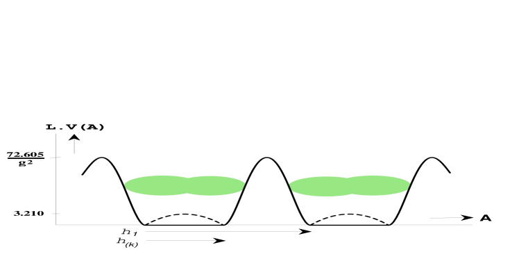
Figure 4: Sketch of the potential for the torus. Shown are two vacuum valleys, related to each other by a gauge transformation $h_{1}$, with winding number $\nu(h_{1})=1$. The induced one-loop effective potential, of height $3.210/L$, has degenerate minima related to each other by the anti-periodic gauge transformations $h_{(k)}$. The classical barrier, separating the two valleys, has a height $72.605/Lg^{2}$.

At larger volumes extra degrees of freedom will behave non-perturbatively. We know from the existence of gauge transformations with non-trivial winding number

$$\nu(h)={1\over 24\pi^{2}}\int_{M}\mbox{\,tr\,}((h^{-1}dh)^{3}),$$ (15)

that there exist gauge equivalent vacuum valleys, that can be reached only by crossing a saddle point (called the finite volume sphaleron), see Fig. 4. Typically this saddle point lies on the tunneling path (the instanton), with the euclidean time of the instanton solution playing the role of the path parameter. We expect, as will be shown for the three-sphere, that the boundary of the fundamental domain along this path in field space across the barrier occurs at the saddle point in between the two minima. The degrees of freedom along this tunneling path go outside of the space of zero-momentum gauge fields and if the energy of a state flows over the barrier, its wave functional will no longer be exponentially suppressed below the barrier and will in particular be non-negligible at the boundary of the fundamental domain. Boundary identifications in this direction of field space now become dynamically important too. The relevant “Bloch momentum” is in this case the $\theta$ parameter. Wave functionals pick up a phase factor $e^{i\theta}$ under a gauge transformation with winding number one.

Figure 5: The top figures show $LE(g)$ for the relevant (positive parity) representations. The dotted lines are without the two loop correction included. The dashed curve denotes the barrier height $LE_{sph}(g)$. The bottom figures show $z(g)=Lm(g)=L(E(g)-E_{0}(g))$, and the dashed line is at $z=2\pi$.

To estimate for which volumes the extra degrees of freedom start to contribute non-perturbatively, the minimal barrier height that separates two vacuum valleys was found to be $E_{sph}(g)=72.605/Lg^{2}$, using the lattice approximation and carefully taking the continuum limit.[33] As long as the states under consideration have energies below this value, the transitions over this barrier can be neglected (or treated semi-classically if there is no perturbative contribution) and the zero-momentum effective hamiltonian provides an accurate description. One can now find for which volume the energy starts to be of the order of this barrier height. For this purpose we have collect the energy levels as a function of $g$ in Fig. 5. In the top two figures we have plotted $LE(g)$ for the various representations of interest (0 stands for the vacuum state, which is in the $A_{1}^{+}$ representation of the cubic group). The dotted curves are without the two loop corrections included. In the same figures the dashed curve shows the height of the instanton barrier. In the lower two figures we show $z=Lm\equiv L(E-E_{0})$. The dashed line is at $z=2\pi$. We see that the sensitivity to the two loop corrections almost entirely drops out for the energy differences, at the scale of this figure. We now read off that instantons only become important for $z_{0}=5$ to 6, i.e. for $L$ roughly 5 to 6 times the correlation length set by the scalar glueball mass. Certain states may actually be less sensitive to instantons, in case the representation is such that the wave functional in the direction of the barrier is suppressed. This may for example be the case for the $T_{2}^{+}$ state. It should also be noted that $z=2\pi$ is associated with the energy scale $2\pi/L$ of the non-zero momentum field modes that have been integrated out. Therefore, $z$ should also not be much bigger than $2\pi$, although also here the particular representation may matter.

On the three-torus we have therefore achieved a self-contained picture of the low-lying glueball spectrum in intermediate volumes from first principles with no free parameters, apart from the overall scale. For very small volumes the energy of electric flux vanish and there is an accidental rotational symmetry, only split by the $\mbox{$\cal O$}\left(g^{8/3}\right)$ terms in Eq. (3). The $2^{+}$ tensor glueball splits in a nearly degenerate doublet $E^{+}$ and a triplet $T_{2}^{+}$. Both are lighter than the scalar $0^{+}$, also denoted by $A_{1}^{+}$ as the scalar singlet representation of the cubic group. Going to larger volumes, $L>0.1$ fermi, the energy of electric flux per unit length, which in an infinite volume would be the string tension $K$, is surprisingly constant in intermediate volumes, whereas the splitting of the tensor states becomes quite large. In intermediate volumes the doublet $E^{+}$ and triplet $T_{2}^{+}$ have respectively masses of roughly 0.9 and 1.7 times the scalar mass. This doublet $E^{+}$, lighter than the scalar, was first observed in the lattice studies of Berg and Billoire,[34] and caused some stir at the time.

The lattice data for the triplet [35] were obtained only after our continuum results first appeared [23, 18] and did not confirm the predictions for this state. This was resolved by Vohwinkel [32] by observing that the state we had initially identified as $T_{2}^{+}$ (taking $p_{1}=p_{2}=p_{3}=1$ instead of $p_{1}=-p_{2}=-p_{3}=1$) actually carried two units of electric flux (cmp. Eq. (13)), making it even more of a surprise that it was found to be even lighter than the doublet $E^{+}$ in intermediate volumes. In the infinite volume limit it is pushed out of the low-lying spectrum. Around the same time this state (named $T_{11}$) was as such measured on the lattice,[36] confirming the proper interpretation of these states.

Electric flux energies (for the trivial representation) are labelled by $e=e_{1}$ for ${\bf e}=(1,0,0)$, $e_{2}$ for $(1,1,0)$ and $e_{3}$ for $(1,1,1)$. For $e_{n}$ we speak of $n$ units of electric flux, sometimes called “torelon” energies. As was argued by ’t Hooft,[9] if a confining string would have formed, $E_{e}=KL$ (or $z_{e}=LE_{e}=KL^{2}$), it would be energetically favorable to run along the direction of ${\bf e}$, giving $R_{n}\equiv E(e_{n})/E(e_{1})=\sqrt{n}$, instead of splitting in separate strings, each winding in the direction for which $e_{j}=1$, which would give $R_{n}=n$. In intermediate volumes it is the latter behavior that we found,[23] confirmed by Monte Carlo results.[37] One has to go to quite large volumes to start to observe the expected $\sqrt{n}$ behavior.[38] The same is found for SU(3), in a study where a different lattice Monte Carlo method was used to get the electric flux energies.[39]

Figure 6: Left: The ratio $\sqrt{K(L)}/m_{E}$ as a function of $z_{E}=m_{E}(L)L$. Full (continuum), dashed-dotted ($6^{3}$ lattice) and dashed ($4^{3}$ lattice) curves give the hamiltonian results. Rayleigh-Ritz diagonalization errors are smaller than the thickness of the lines. The sensitivity to the two loop correction can be read off from the dotted curve ($4^{3}$ lattice), where this correction was not included. Note the blown-up scale. Right: electric flux ratios $R_{n}$ as a function of $z_{e}=E_{e}(L)L$. Monte Carlo data [37, 40] obtained with the Wilson action on a $N^{3}\times N_{t}$ lattice ($N_{t}>6N$), for $N=4$ (dots), 6 (squares), 8 (triangles) and 10 (diamond).

The lattice Monte Carlo data of Berg and Billoire [37, 40] are compared with the hamiltonian results in Fig. 6. On the left we show the ratio $\sqrt{K(L)}/z_{E}$ as a function of $z_{E}$. Their methods had considerable difficulty in dealing with the scalar glueball state, since it has the same quantum numbers as the vacuum. To push the results to low values of $z_{E}$, they used lattices $N^{3}\times N_{t}$ with $N_{t}=256$ for $N=4$. Please note that $z=m_{E}L$ around 0.95 is nearly a constant (even not single valued) function of $g(L)$, see Fig. 5. This over-emphasizes the steep behavior where the wave function starts to spread over the whole vacuum valley, leading to non-zero energies of electric flux. We took the Monte Carlo data from Table V of their paper,[40] but removed those entries with $N_{t}/N\leq 6$. On the right in Fig. 6 we compare with the lattice Monte Carlo data of Berg [37] for the electric flux ratios, but used where available, the more accurate results [40] for $z_{e}=LE_{e}$. The data at $\beta=4/g_{0}^{2}=2.7$ from both papers [37, 40] were left out because they were not consistent with each other.

Considerable progress was achieved by the so-called variational method, which allowed much more accurate results, not only for the scalar glueball, but also for arbitrary other representations.[35] In Fig. 7 we present a comparison with the Monte Carlo results of Michael,[41] obtained for a lattice of spatial size $4^{3}$, confirmed in a study of improved lattice actions.[42] The hamiltonian results below $z=0.95$ are due to Lüscher and Münster,[31] which is where the spectrum is insensitive to any identifications at the boundary of $\Lambda$. The electric flux energy ratios $R_{2}$ and $R_{3}$ are shown on the right, cmp. Fig. 6.

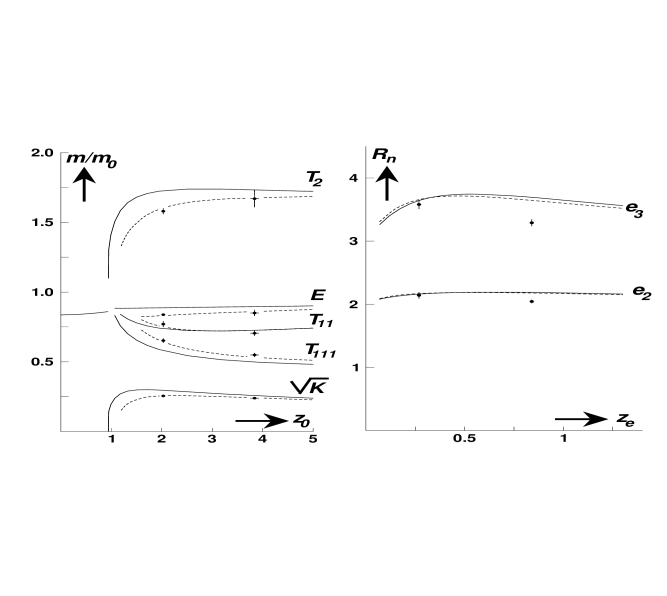
Figure 7: Left: mass ratios $m/m_{0}$ as a function of $z=m_{0}(L)L$, with $m_{0}$ the scalar glueball mass. Full (continuum) and dashed ($4^{3}$ lattice) curves give the hamiltonian results. Shown are string tension $\sqrt{K(L)}$, $E^{+}$ and $T_{2}^{+}$ tensor masses and the exotic states $T_{11}$ with two, and $T_{111}=T_{2}(111)$ with three units of electric flux. Right: electric flux ratios $R_{n}$ as a function of $z_{e}$. Monte Carlo data [41] obtained with Wilson action on $4^{3}\times N_{t}$ lattice ($N_{t}=32,\beta=2.4$ and $N_{t}=99,\beta=3.0$).

We note that the solid curves that represent the continuum results, which were reproduced by Berg and Vohwinkel,[43, 44] deviate significantly from the lattice data. Initially the lattice data were not accurate enough to show this deviation. Even though one should not expect a $4^{3}$ lattice to be an accurate approximation for the continuum, it was cause for some doubt that the approximations made in the continuum studies were not under control as well.[40] To settle this issue we redid the complete derivation of the effective hamiltonian starting from the lattice theory, without taking the continuum limit.[45, 25] The hamiltonian is basically of the same form as in Eq. (3), except that the coefficients in Eq. (11) depend on the lattice spacing (some extra corrections appear, e.g. to correct for the discrete time evolution). One can follow the renormalization group flow of the hamiltonian to its continuum fixed point in this formalism in all detail, see Fig. 8. Using the same analysis as in the continuum leads for a finite lattice to the dashed curves in

Figure 8: Flow of the lattice hamiltonian coefficients to their continuum ($N\rightarrow\infty$) values. Shown are $\alpha_{i}(N)/\alpha_{i}$ (dashed lines) and $\gamma_{i}(N)/\gamma_{i}$ (full lines) as a function of the square of the lattice spacing $(a/L)^{2}=1/N^{2}$.

Figs. 6,7. The lattice data now agree perfectly, up to a volume of about 0.75 fermi, the regime for which we have shown that the effective hamiltonian in the zero-momentum modes should provide a good approximation. The deviations for $R_{2}$ and in particular for $R_{3}$ are in accordance with the fact that these are of relatively high energy, and therefore expected to be sensitive to other non-perturbative effects that invalidate integrating out all the non-zero momentum modes, see Fig. 5.

3.1 General Gauge Group

The question of extending the previous results to SU(3) is a natural one in the light of QCD. The perturbative expansion,[7, 46] vacuum-valley effective potential,[7, 30] and the semi-classical evaluation of the energy of electric flux [47] (due to the tunneling through the quantum induced vacuum-valley effective potential) are more or less straightforward. The non-trivial problem of formulating the appropriate boundary conditions on the boundary of the fundamental domain for SU(3) was solved by Vohwinkel and qualitative agreement with the lattice data was found.[48, 44] With the results for SU(3) in hand generalization to SU($N$) was achieved.[49] The formalism sketched in Sec. 2 was not yet developed in those early days. What is now called the fundamental domain was then called the unit cell. Although the argumentation was more cumbersome, the underlying principles were the same.

A simple approximation for Lüscher’s effective hamiltonian in terms of the zero-momentum gauge fields $A_{j}({\bf x})=ic_{j}^{a}T_{a}/L$ ($T_{a}$ the hermitian generators of SU($N$) and $f_{ij}\equiv L^{2}F_{ij}({\bf x})$ the dimensionless field strength) is given by

$$H_{{\rm eff}}(c)={-g^{2}\over 2L(1+\alpha_{1}g^{2})}\sum_{i,a}{\partial^{2}\over\partial{c_{i}^{a}}^{2}}-{1\over 2L}({1\over g^{2}}+\alpha_{2})\sum_{i,j}\mbox{\,tr\,}(f_{ij}^{\,2})+V_{1}(c),$$ (16)

with

$$V_{1}(c)={2\over L}\sum_{{\bf p}\neq{\bf 0}}\left(\sqrt{\mbox{\,Tr\,}_{{\rm ad}}(2\pi{\bf p}+{\bf c}^{a}{\rm ad}\,T_{a})^{2}}-\sqrt{\mbox{\,Tr\,}_{{\rm ad}}(2\pi{\bf p})^{2}}\right),$$ (17)

where $g$ is the renormalized coupling constant at the scale $\mu=1/L$. In a perturbative expansion,[7, 46] this gives the correct result up to $\mbox{$\cal O$}\left(g^{8/3}\right)$. Along the vacuum valley, parametrized by $A_{j}({\bf x})=i\sum_{b=1}^{N-1}C_{j}^{b}T_{b}/L$, where the first $N-1$ generators are assumed to commute (forming a basis of the Cartan subalgebra $H_{G}$), the effective potential $V_{1}(c)$ is exact to one loop order. A more explicit result can be found in Sec. 3.2, Eq. (25). As for SU(2), one does not include the ${\bf p}={\bf 0}$ term, since only the non-zero momentum modes are to be integrated out.

The effective potential $V_{1}(c)$ only depends on the Casimir invariants

$$r_{i}^{2}=2\mbox{\,tr\,}[(c_{i}^{a}T_{a})^{2}]\,,\quad s_{i}=4\mbox{\,tr\,}[(c_{i}^{a}T_{a})^{3}]\,,\quad\cdots,$$ (18)

where the sum over all color indices is implicit. There are as many independent Casimir invariants as the rank of the gauge group. For SU(2) only $r_{i}$ will be non-trivial. These coordinates are uniquely related to those obtained by restricting the zero-momentum gauge field to be abelian. For SU(2), $c_{i}^{a}T_{a}=C_{i}\tau_{3}/2$ yields $r_{i}^{2}=C_{i}^{2}$, whereas for SU(3), in terms of the Gell-Mann matrices, $c_{i}^{a}T_{a}=(C^{1}_{i}\lambda_{8}+C^{2}_{i}\lambda_{3})/2$ gives $s_{i}=C^{1}_{i}\sqrt{3}((C^{2}_{i})^{2}-(C^{1}_{i})^{2}/3)$ and $r_{i}^{2}=(C^{1}_{i})^{2}+(C^{2}_{i})^{2}$. In this manner the effective potential on the set of abelian zero-momentum modes can indeed be minimally extended in a unique way to all constant gauge fields.

By adding the zero-momentum (${\bf p}={\bf 0}$) contribution to the one-loop effective potential,

$$V_{{\rm eff}}(c)=V_{1}(c)+2L^{-1}\sqrt{\mbox{\,Tr\,}_{{\rm ad}}[({\bf c}^{a}T_{a})^{2}]}\,,$$ (19)

restricted to the vacuum valley gives the appropriate effective potential when integrating out all the field modes orthogonal to the vacuum valley. Its symmetries are a consequence of gauge invariance, which can be divided in two classes. The constant gauge transformations, that leave $H_{G}$ invariant. This is represented by the Weyl group $\cal W$ acting on ${\bf C}^{b}$ (for SU(2) ${\bf C}\rightarrow-{\bf C}$). The other class of gauge transformations that leaves the set ${\bf C}^{b}$ invariant are of the form $h_{{\bf\Theta}}({\bf x})=\exp(2\pi i{\bf x}\cdot{\bf\Theta}/L)$, where $\Theta_{i}\in H_{G}$ such that $h$ does not affect the periodic boundary conditions on the gauge fields. These lead to shift symmetries on ${\bf C}^{b}$. The associated lattice of $\Theta_{j}$ corresponds to the dual root lattice $\tilde{\Lambda}_{r}$, as follows from the condition that $\exp(2\pi i\Theta_{j})=1$. The vacuum valley, i.e. the moduli space of flat connections ($F_{ij}=0$), corresponds to the orbifold $[H_{G}/2\pi\tilde{\Lambda}_{r}]^{3}/\mbox{$\cal W$}$. Recently it has become clear that for orthogonal and exceptional Lie-groups there are other, disconnected, components in the moduli space of flat connections, which we will briefly discuss in Sec. 3.5.

A crucial role is played by the twisted gauge transformations, only periodic up to an element of the center $Z_{N}$ of the gauge group.[9] These can be realized with $h_{{\bf\Theta}}$, but now $\Theta_{j}$ belongs to the dual weight lattice $\tilde{\Lambda}_{w}$, which follows from the requirement that $\exp(2\pi i\Theta_{j})$ is an element of the center $Z_{G}$ of the gauge group. Indeed, $\tilde{\Lambda}_{w}/\tilde{\Lambda}_{r}\cong Z_{G}$. These twisted gauge transformations generate a shift symmetry associated with $\tilde{\Lambda}_{w}$. Their homotopy type is specified by ${\bf\Theta}\in(\tilde{\Lambda}_{w}/\tilde{\Lambda}_{r})^{3}\cong Z_{G}^{3}$. A particular representative for SU($N$) is given by $h_{{\bf k}}({\bf x})=\exp(2\pi i{\bf k}\cdot{\bf x}\Theta_{0}/L)$, where $\Theta_{0}\in H_{G}$ is a generator for the center, $\exp(2\pi i\Theta_{0})=\exp(2\pi i/N)$. For SU(2) we can choose $\Theta_{0}=\tau_{3}/2$ and for SU(3) there are two independent choices (that span the dual weight lattice $\tilde{\Lambda}_{w}$) $\Theta_{0}=\lambda_{8}/\sqrt{3}$ and $\Theta_{0}^{\prime}={\scriptstyle{{1\over 2}}}(\lambda_{3}-\lambda_{8}/\sqrt{3})$. The non-trivial homotopy is labelled by ${\bf k}\in Z_{N}^{3}$ and is thus in general non-trivially represented on the wave functionals. Any gauge transformation can be decomposed [50] in $h=h_{\bf k}h_{1}^{\nu}(h)h_{0}$, where $h_{1}$ is a particular strictly periodic gauge transformation with unit winding number, $\nu(h_{1})=1$. What is left is a homotopically trivial gauge function $h_{0}$, under which the wave functional is invariant. We therefore have

$$\Psi([h]A)=\Psi([h_{{\bf k}}h_{1}^{\nu}]A)=\exp(2\pi i{\bf e}\cdot{\bf k}/N)\exp(i\theta\nu)\Psi(A),$$ (20)

where $\theta$ is the usual vacuum parameter associated with instantons and ${\bf e}$ (defined modulo $N$) is the gauge invariant definition of electric flux.[9] As for SU(2) the electric flux quantum number can be implemented within the zero-momentum effective hamiltonian by imposing suitable boundary conditions on the boundary of the fundamental domain. For this we study the action of $h_{{\bf k}}$ on ${\bf C}^{b}$, corresponding to a shift. For SU(2) ${\bf C}\rightarrow{\bf C}+2\pi{\bf k}$ and for SU(3) $({\bf C}^{1},{\bf C}^{2})\rightarrow({\bf C}^{1}+2\pi(2{\bf n}-{\bf l})/\sqrt{3},{\bf C}^{2}+2\pi{\bf l})$, with ${\bf k}={\bf n}+{\bf l}$ (mod 3) specifying the homotopy type of the gauge transformation.

Fig. 9 gives for SU(3) the equipotential lines of the effective potential $V_{{\rm eff}}$, in a plane specified by putting $C_{2}^{b}=C_{3}^{b}=0$, the fundamental domain $\Lambda$ (bounded by the dashed hexagon) and the Gribov region $\Omega$ (bounded by the fat hexagon). The triangular lattice structure is due to the invariance under twisted gauge transformations and reflects the dual weight lattice of SU(3). Indeed, the gauge transformations $\exp(2\pi i\Theta_{0}x_{j}/L)$ and $\exp(2\pi i\Theta_{0}^{\prime}x_{j}/L)$ all map points on the boundary of the fundamental domain to the same boundary. They also map ${\bf C}^{b}=0$ to the Gribov horizon. The Weyl transformations are generated by the reflections in the three principle axes of the dual weight lattice.

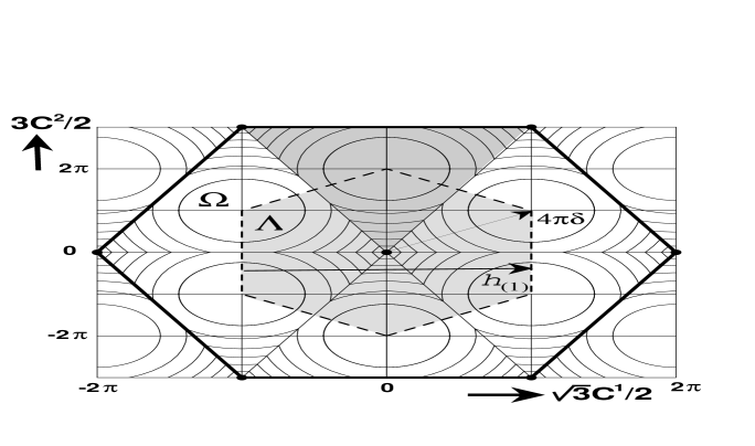
Figure 9: Two dimensional cross-section of $V_{{\rm eff}}$, for $C_{1}^{b}T_{b}=C_{1}^{1}\lambda_{8}/2+C_{1}^{2}\lambda_{3}/2$ and $C_{2,3}^{b}=0$. The circles indicate the equipotential lines (in increments of $V_{{\rm eff}}(4\pi\delta)/7$). The light shaded area represents the fundamental region, with the dashed hexagon as its boundary, the fat hexagon indicates the Gribov horizon, with gauge copies of $A=0$ indicated by the dots. The darker shaded area is the so-called fundamental Weyl chamber.

The near spherical behavior of the equipotential lines within each triangle is due to a remarkably accurate approximation (cmp. Fig. 10) that holds for any SU($N$) when restricting $C_{i}^{b}$ to one dimension, say $C_{1}^{b}=C^{b}$ (normalizing as usual $\mbox{\,tr\,}(T_{a}T_{b})={\scriptstyle{{1\over 2}}}\delta_{ab}$)

$$V_{{\rm eff}}(C)\approx N\left((4\pi\delta)^{2}-(C-4\pi\delta)^{2}\right)/2\pi L,$$ (21)

for $C$ in the Weyl chamber restricted to the fundamental domain, centered around $4\pi\delta$, where $\delta$ is the highest weight. For SU(2) $\delta=1/4$ and for SU(3) $\delta=(\delta^{1},\delta^{2})=(\sqrt{3},1)/6$. It is also instructive from Fig. 9 to identify the orbifold singularities, along the axes of the dual weight lattice (edges of the Weyl chambers), which are fixed under the Weyl reflections. This is where the $U(1)^{2}$ symmetry in a generic point of the vacuum valley is restored to SU(2), whereas at the corners (all gauge copies of $A=0$) the full SU(3) symmetry is restored. At these locations also some of the directions in which the classical potential is quadratic turn quartic. It is this that gives rise to the conic singularities in $V_{{\rm eff}}$. The effective potential $V_{1}$ in Eq. (17), when restricted to the fundamental domain, is free from any of these singularities, since they are caused by fluctuations in the non-abelian constant modes, which are not integrated out in Eq. (17). The conic singularities of $V_{{\rm eff}}$ in $\Lambda$ are therefore all described by $2L^{-1}\sqrt{\mbox{\,Tr\,}_{{\rm ad}}[({\bf C}^{b}T_{b})^{2}]}=2NL^{-1}|\delta_{b}{\bf C}^{b}|$, see Eq. (19).

To implement the symmetries on the wave functional we perform a change of coordinates $c_{i}^{a}\rightarrow(C^{b}_{i},\Omega_{i})$, where $\Omega_{i}$ stands for the collection of SU($N$)-angular coordinates parametrizing SU($N$)/U$(1)^{N-1}$ and $(C^{a}_{i})$ are restricted to a fundamental Weyl chamber, for SU(3) the triangular shaded region in Fig. 9, where the relation between $(C^{1},C^{2})$ and $(r,s)$ is one to one. For SU(2) these new coordinates are the spherical coordinates $(r_{i},\Omega_{i})$, with $\Omega_{i}=(\theta_{i},\phi_{i})$ coordinates on $S^{2}=SU(2)/U(1)$. The square root of the Jacobian of this transformation, is given by $J=\prod_{i}J_{i}$, with $J_{i}=C_{i}$ for SU(2) and $J_{i}=C^{2}_{i}((C^{2}_{i})^{2}-3(C_{i}^{1})^{2})$ for SU(3). The wave functions can be decomposed as

$$\Psi(c)=\prod_{i}J_{i}^{-1}(C_{i}^{b})\chi_{i}^{\vphantom{\dagger}}(C_{i}^{b})\mbox{$\cal Y$}_{i}(\Omega_{i}).$$ (22)

The “radial” part $\chi$ will be antisymmetric with respect to Weyl reflections, so as to cancel the zero’s of the Jacobian. For SU(2) the angular wave functions $\mbox{$\cal Y$}(\Omega)$ are nothing but the spherical harmonics, see Eq. (14), whereas in general they are irreducible representations of the gauge group. Helpful in making suitable choices for $\chi$ is that the vacuum valley kinetic term after the rescaling with the square root $J$ of the Jacobian becomes $-{\scriptstyle{{1\over 2}}}g^{2}\sum_{i,a}(\partial/\partial C_{i}^{a})^{2}$, compatible with the canonical flat metric on the orbifold. Furthermore, as is familiar from the radial reduction in three dimensions, this rescaling does not create an additional potential term, since $J$ is in all cases harmonic, $\sum_{i,a}\partial^{2}J/(\partial C_{i}^{a})^{2}=0$.

We note that suitable combinations of a shift and Weyl reflection leave invariant the lines that constitute the polygon at the boundary of the fundamental domain, see Figs. 3 and 9. This implies that alternatively the properties of $\chi$ can be described in terms of boundary conditions at the boundary of the fundamental domain. E.g., for SU(2) this leads to two possible choices of boundary conditions at $r_{j}=\pi$, for each $j$, see Eq. (13). One can use $\chi(C)=\sin(nC/2)$, although spherical Bessel functions provide a more efficient choice, keeping the hamiltonian more sparse.[18] Carefully working out the consequences of the symmetries one can show [48, 49] that a complete basis for $\chi$ in the case of SU(3) is given by

$$\chi(C^{1},C^{2}) = \sin\left(mC^{2}/2\right)\exp\left(inC^{1}\sqrt{3}/2\right)$$

$$+ \sin\left(m(\sqrt{3}C^{1}-C^{2})/4\right)\exp\left(in\sqrt{3}(\sqrt{3}C^{1}+C^{2})/2\right)$$

$$- \sin\left(m(\sqrt{3}C^{1}+C^{2})/4\right)\exp\left(in\sqrt{3}(\sqrt{3}C^{1}-C^{2})/2\right),$$

for each of the three coordinate directions. The quantum numbers $n$ and $m$ will be restricted by the electric flux and irreducible representations of the Weyl and cubic groups, which is the part that requires most of the care. Finally if one restricts $\prod_{i}\mbox{$\cal Y$}_{i}$ to transform as a singlet under SU($N$) one obtains a complete and gauge invariant basis for the effective hamiltonian, that through the boundary conditions carries the information of electric flux. Needless to say that for SU(3) the computation of all the relevant matrix elements [48] is rather more cumbersome than for SU(2). However, once the matrix of the hamiltonian for a particular basis is computed one performs a simple Rayleigh-Ritz analysis to determine the spectrum. The region where the wave functional spreads out over the whole vacuum valley, with the energy of electric flux no longer suppressed by the quantum induced barrier of $V_{{\rm eff}}$, is well described by this Rayleigh-Ritz analysis, based on Eq. (3.1). Of course, also for SU(3) the results are valid as long as the classical barrier is sufficiently high as compared to the energy-levels studied, cmp. Fig. 4. Like for SU(2) the approximations break down for $L$ large than 5 to 6 times the correlation length of the scalar glueball. That beyond this volume, $L\sim 0.75$ fermi, instanton effects set in can be seen from the rather sudden onset of the topological susceptibility.[51]

3.2 Including Massless Quarks

Quarks fields are not invariant under the center of the gauge groups. This means that on the space of zero-momentum abelian gauge fields, which still form the classical vacuum valley, the twisted gauge transformations no longer represent a symmetry. This complicates matters since without the equivalence under twisted gauge transformations the fundamental domain extends to the Gribov horizon. Some of these complications may be avoided by introducing on the original fundamental domain additional quark fields, obtained by applying a twisted gauge transformation. The boundary identification on the boundary of the fundamental domain are include an operation that permutes these fermion field components. This has not been worked out so far.

Nevertheless, interesting statements can be made about the vacuum structure in small enough volumes, for which the wave functional is sufficiently localized around the vacuum configuration. One simply adds in one loop order the quantum effects of the quark field fluctuations. The resulting effective potential will no longer respect the center symmetry, but it still properly reflects invariance under constant and periodic gauge transformations. The quark fields can satisfy either periodic or anti-periodic spatial boundary conditions. Actually, for SU(2) (with $-1$ a non-trivial element of $Z_{2}$) these are equivalent by a twisted gauge transformation with homotopy type ${\bf k}=(1,1,1)$. Under this gauge transformation the gauge field is shifted and shows it is not a priori clear that $A=0$ will represent the proper classical vacuum to expand around. As we will show, it will be the correct one only with anti-periodic boundary conditions for the quark fields, both for SU(2) and SU(3). In that case, due to the anti-periodicity, there will be no zero-energy modes for the quark fields, and chiral symmetry is unbroken in the finite volume. For SU(3) no gauge equivalence of periodic to anti-periodic boundary conditions holds, and the vacuum structure with periodic quark fields actually leads to spontaneous breaking of some discrete symmetries. Yet, no zero-energy quark modes appear, and chiral symmetry remains unbroken. It also means that in a small volume, with quark momenta of the order $\pi/L$ and glueball masses of order $g^{2/3}(L)/L$, that glueballs cannot decay in mesons. The quark degrees of freedom can be integrated out.

Figure 10: Vacuum-valley effective potential at $C_{2}=C_{3}=2\pi$ for SU(2) and two flavors of periodic massless quarks (Eq. (25) with ${\bf k}={\bf 0}$), normalized to 0 at its minimum, as well as the effective potential for zero flavors (Eq. (8)). The dashed curve represents Eq. (21).

To be more specific let us first generalize the computation of the vacuum-valley effective potential to include the quark field fluctuations. The most efficient way to represent the result is to introduce the weight vectors $\mu^{(i)}$, determined by the eigenvalues of the abelian generators,

$$T_{b}={\rm diag}(\mu^{(1)}_{b},\mu^{(2)}_{b},\cdots,\mu^{(N)}_{b}),\quad T_{b}\in H_{G}.$$ (24)

For SU(2) one finds $\mu^{(1)}={\scriptstyle{{1\over 2}}}(1,-1)$, whereas for SU(3) $\mu^{(1)}=(1,1,-2)/\sqrt{12}$ and $\mu^{(2)}={\scriptstyle{{1\over 2}}}(1,-1,0)$ (the conventions used in this paper are $T_{1}={\scriptstyle{{1\over 2}}}\lambda_{8}$ and $T_{2}={\scriptstyle{{1\over 2}}}\lambda_{3}$). With $n_{f}$ flavors of massless quark fields we find [19] (see Fig. 10)

$$V_{{\rm eff}}^{{\bf k}}({\bf C}^{b})=\sum_{i>j}V({\bf C}^{b}[\mu^{(i)}_{b}-\mu^{(j)}_{b}])-n_{f}\sum_{i}V({\bf C}^{b}\mu^{(i)}_{b}+\pi{\bf k}),$$ (25)

with ${\bf k}={\bf 0}$ or ${\bf k}=(1,1,1)$, for resp. periodic or anti-periodic boundary conditions on the quark fields. The function $V({\bf C})$ is the SU(2) one-loop effective potential for $n_{f}=0$, Eq. (8). The correct quantum vacuum is to be found at the minimum of this effective potential.

Observe that the gauge symmetry should not be spontaneously broken, which implies that the Polyakov loop observables

$$P_{j}({\bf x})\equiv\frac{1}{N}\mbox{\,tr\,}\left(P\exp\,(\int_{0}^{L}ds\,A_{j}({\bf x}+s{\bf e}^{(j)})\right),$$ (26)

should be a constant center element at the vacuum configurations, or

$$P_{j}=\frac{1}{N}\mbox{\,tr\,}\left(\exp(iC_{j}^{b}T_{b})\right)=\frac{1}{N}\sum_{n}\exp(i\mu^{(n)}_{b}C^{b}_{j})=\exp(2\pi il_{j}/N).$$ (27)

This implies that $\mu^{(n)}_{b}{\bf C}^{b}=2\pi{\bf l}/N$ (mod $2\pi$), independent of $n$, and gives $V_{{\rm eff}}^{{\bf k}}=-n_{f}NV(2\pi{\bf l}/N+\pi{\bf k})$. In the case of anti-periodic boundary conditions, ${\bf k}=(1,1,1)$, this is minimal only when ${\bf l}={\bf 0}$ (mod $2\pi$). This means the quantum vacuum in this case is the naive one, $A=0$ ($P_{j}=1$). In the case of periodic boundary conditions, ${\bf k}={\bf 0}$, the above candidate vacua have ${\bf l}\neq{\bf 0}$, that is $P_{j}$ correspond to non-trivial center elements. Both for SU(2) and SU(3) this means $l_{j}=\pm 1$. For SU(2) the vacuum with $P_{j}=-1$ is unique, as also follows from the gauge equivalence argument given above. The only difference is that one now needs to expand around ${\bf C}=2\pi(1,1,1)$. For SU(3), however, there are now 8 possible choices $P_{j}=\exp(\pm 2\pi i/3)$, related by the three coordinate reflections. As this is a symmetry of the full hamiltonian, each is indeed equivalent. But it does mean that in a small volume parity (P) and charge conjugation (C) are spontaneously broken, although CP is still a good symmetry.[19] A consequence of the spontaneous breaking of parity is that the mass gap, the lowest excitation above the vacuum, is exponentially small in a small volume. All these intricate effects would make this an ideal testing ground for dynamical fermion algorithms in lattice gauge theory.

The minima of the effective potential are obtained from $A=0$ by the twisted gauge transformation $h_{{\bf l}}({\bf x})$. As there are no zero-energy quark field modes, also the effective hamiltonian can be expressed as in the bosonic case in terms of the zero-momentum gauge fields, after taking this shift into account. In the case of SU(3) with periodic boundary conditions, because of the spontaneous break down of parity and charge conjugation invariance, extra terms appear in Lüscher’s effective hamiltonian. To the order in which this hamiltonian was worked out the new interaction $\mbox{\,tr\,}(\{A_{i},A_{j}\}A_{k})$ appears. In addition couplings that were equal because they were related by the discrete symmetries, now spontaneously broken, will split.[19] All these corrections are linear in the number ($n_{f}$) of quark flavors. The flavor dependence of the effective hamiltonian for the case of anti-periodic boundary is simpler, since no new couplings appear. For SU(2) one simply replaces $\alpha_{i}$ and $\gamma_{i}$ in Eq. (3) by $\alpha_{i}-2n_{f}\alpha_{i}^{\prime}$ and $\gamma_{i}-2n_{f}\gamma_{i}^{\prime}$, with

$$\gamma_{1}^{\prime}=-2.1272012\cdot 10^{-2}, \alpha_{1}^{\prime}=+3.098211\cdot 10^{-5},$$

$$\gamma_{2}^{\prime}=+4.2255250\cdot 10^{-4}, \alpha_{2}^{\prime}=+1.7211922\cdot 10^{-3},$$

$$\gamma_{3}^{\prime}=-7.3994300\cdot 10^{-4}, \alpha_{3}^{\prime}=+3.0178786\cdot 10^{-5},$$

$$\gamma_{4}^{\prime}=-2.8659656\cdot 10^{-6}, \alpha_{4}^{\prime}=+3.2156523\cdot 10^{-5},$$

$$\gamma_{5}^{\prime}=+1.1578663\cdot 10^{-5}, \alpha_{5}^{\prime}=-3.2271736\cdot 10^{-5},$$

$$\gamma_{6}^{\prime}=-7.9447492\cdot 10^{-5}.$$ (28)

Independently Kripfganz and Michael calculated for SU($N$) to $\mbox{$\cal O$}\left(g^{8/3}\right)$ the change in the coefficients of Lüscher’s effective hamiltonian, due to quarks with anti-periodic boundary conditions only.[52] They confirmed the values in Eq. (28) and also introduced for SU(2) a lagrangian formulation of the effective hamiltonian in terms of compact group variables, that incorporates in a simple way the proper boundary conditions in field space.[36] After full equivalence was established,[53, 54] the Monte Carlo analysis of this effective lagrangian model continued to suffer from a technical difficulty in efficiently implementing the kinetic term,[41] only fully understood by Vohwinkel a number of years later.[55] This has hampered using the lagrangian formulation as a reliable alternative [56] for the hamiltonian Rayleigh-Ritz analysis.

There is another choice of boundary conditions that strongly reduces the center symmetry. This is called C periodic boundary conditions, where the field is periodic up to a charge conjugation. The boundary conditions can be used to avoid the system to be charge neutral, as is the case for periodic boundary conditions, both for magnetic and electric charge. This was the original motivation to introduce these boundary conditions for the abelian theory,[57] which were subsequently studied for non-abelian gauge theories.[58] For SU(2), which is pseudo real, one retrieves the periodic case, but for SU(3) the center symmetry is completely broken and a number of the features we saw when including quark fields, appear here as well. The vacuum valley for SU(3) is reduced from six to three dimensional in terms of the real gauge field ${\bf A}={\scriptstyle{{1\over 2}}}i{\bf C}\lambda_{2}/L$, with [59]

$$V_{{\rm eff}}({\bf C})=V({\scriptstyle{{1\over 2}}}{\bf C})+V({\bf C}-\pi{\bf l})+V({\scriptstyle{{1\over 2}}}{\bf C}-\pi{\bf l}),$$ (29)

where $V({\bf C})$ is the SU(2) effective potential, see Eq. (8), and ${\bf l}=(1,1,1)$. The minimum of this effective potential occurs at the four points ${\bf C}=(\pi,\pi,\pi)$, $(-\pi,-\pi,\pi)$, $(\pi,-\pi,-\pi)$, and $(-\pi,\pi,-\pi)$, which correspond to orbifold singularities with quartic modes (associated with the three real generators $i\lambda_{A}/2$, for $A=2$, 5 and 7, forming an SU(2) subalgebra). The effective hamiltonian is again of the Lüscher type, at $\mbox{$\cal O$}\left(g^{2/3}\right)$ identical to it, at higher order additional couplings appear because of the spontaneous breaking of parity, i.e. the cubic group is broken down to the permutation group. No attempts have been made to study the fundamental domain for this theory, and we may expect similar difficulties as in the presence of quark fields.

3.3 The Renormalized Coupling

We have assumed there is a renormalized coupling in terms of which perturbation theory in the field modes that are integrated out is well-behaved. By expressing quantities in dimensionless combinations, lattice Monte Carlo results and continuum (or lattice) hamiltonian results can be compared without being sensitive to any problems in expressing the renormalized coupling in terms of the bare coupling. Determining the renormalized strong coupling constant non-perturbatively in a reliable way is, however, an important problem. The integration constant of the beta-function, the so-called Lambda parameter, ideally should be fixed in terms of the infrared quantities of the theory, like the mass gap and string tension, or other observables in the low-lying spectrum of the theory. The running of the coupling allows one to compute unambiguously the strong coupling constant at, say the Z-boson mass. The most accurate such method is based on a finite volume study, proposed by Lüscher,[60] long before it was feasible to be implemented.[61] It makes use of a discrete version of the beta-function, the so-called step scaling function. The scale at which the renormalized coupling is defined is fixed by the volume. The volume is subsequently changed by an integer factor (usually, but not necessarily) of 2. So instead of an infinitesimal scale transformation it considers a finite one. The change in the coupling can of course be obtained by intergrating the beta-function, but this function is not available non-perturbatively. Instead, one picks a suitable definition of the renormalized coupling constant at the scale $L$, set by a given physical volume, than doubles $L$ and calculates the value of the coupling at this new scale $2L$. This can all be performed on the lattice (hence the integer scaling factor) using Monte Carlo calculations, at each step carefully extrapolating to the continuum limit. Also (euclidean) time is taken finite, $T=L$. Small volumes go together with high temperatures in such geometries. The naive strategy of taking $L$ large, and defining an observable set by a variable scale within the same finite volume, fails because the lattice spacing gives a limit to the shortest distance one can probe in a given volume, due to computer limitations.

Many definitions of the renormalized coupling could in principle be used, but technical requirements have led to a particular one that is related to the effective action in the background of a constant chromo-electric field, based on the so-called Schrödinger functional [62] (SF). In the spatial directions the boundary conditions are periodic, but in the (finite) time direction one prescribes an initial and a final configuration of gauge fields taking values in the vacuum valley.[62, 8]

$${\rm SU(2)}: C_{j}(t=0)=2\pi\delta+2\eta,\quad C_{j}(t=T)=2\pi-C_{j}(t=0),$$

$${\rm SU(3)}: (C^{1}_{j},C^{2}_{j})(t=0)=2\pi\delta+(-\sqrt{3}\eta,0),$$

$$(C^{1}_{j},C^{2}_{j})(t=T)=(4\pi/\sqrt{3},0)-(C^{1}_{j},C^{2}_{j})(t=0),\quad\forall j,$$

with $\delta$ the highest weight, defined below Eq. (21). The classical equations of motion lead to a linear interpolation in time, giving rise to a constant chromo-electric background. The euclidean quantum effective action, $\Gamma(\eta)$, describes the reaction of the system to this background. The renormalized coupling is defined by $g^{2}(L)=\frac{d\Gamma(\eta)}{d\eta}/\frac{d\Gamma_{0}(\eta)}{d\eta}$ evaluated at $\eta=0$, where $\Gamma_{0}(\eta)$ is the bare effective action. This background has been chosen to stay well away from the orbifold singularities along the vacuum valley for the entire classical path that interpolates between the initial and final configuration, to simplify the perturbative analysis (in part for estimating the lattice artifacts). This particular choice of coupling fits extremely well to the perturbative running of the coupling constant up to the largest volume probed,[8] with $L$ up to $\sim$0.35 fermi. At large volumes the non-perturbative running is bound to deviate.

An alternative definition for the non-perturbatively defined running coupling for SU(2) has been based on ratios of the expectation values of suitable Polyakov loop operators, using twisted boundary conditions,[9] the so-called twisted Polyakov (TP) scheme.[63] We will see next that twisted boundary conditions remove the zero-momentum modes, making perturbation theory well behaved. Without these twisted boundary conditions, computing expectation values in the four dimensional euclidean finite volume is difficult to control.[64] The TP coupling also agrees well with perturbation theory and after matching of the scales, with the SF coupling.[65] Only the largest volume result ($L=0.28$ fermi) probed by the TP coupling lies slightly, but significantly, below the perturbative result. The near perturbative behavior seems to support the fact that non-zero momentum modes do behave perturbatively in intermediate volumes.

3.4 Twisted Boundary Conditions

With twisted boundary conditions, in the absence of zero-momentum modes, the classical vacuum at $A=0$ is isolated and the small volume behavior for the glueball masses is described by a perturbative series in $g^{2}(L)$, as opposed to $g^{2/3}(L)$ in absence of twist. The volume dependence will be quite different, this is in particular true for electric flux energies.[66] Nevertheless, in large volumes the results should not depend on boundary conditions. Therefore, comparing the different boundary conditions gives valuable information about the transition to large volumes. In the hamiltonian formulation the twisted boundary conditions are most easily implemented in a gauge where the so-called twist matrices $\Omega_{j}\in$SU($N$) are constant

$${\bf A}({\bf x}+L{\bf e}^{(j)})=\Omega_{j}^{\dagger}{\bf A}({\bf x})\Omega_{j}.$$ (31)

They satisfy ’t Hooft’s consistency condition,[9] which also gives the relation to the magnetic flux ${\bf m}\in{\rm Z\!\!Z}^{3}_{N}$,

$$\Omega_{k}^{\dagger}\Omega_{\ell}^{\dagger}\Omega_{k}^{\vphantom{\dagger}}\Omega_{\ell}^{\vphantom{\dagger}}=\exp(2\pi i\epsilon_{k\ell j}m_{j}/N).$$ (32)

These generate a so-called Heisenberg group (the group commutator is central, i.e. commutes with all group elements). The finite group theory allows one to construct in an elegant way the most general set $\Omega_{k}\in$SU($N$) for any given ${\bf m}$, and its generalizations to higher dimensions.[67, 68]

It seems that twisted boundary conditions spontaneously break the gauge invariance, due to the explicit choice of $\Omega_{k}$. However, this is of course similar to the case of periodic boundary conditions, which also represents a gauge choice in formulating the boundary conditions. Once one has specified the gauge choice for the boundary conditions, Gauss’s law tells us that local gauge transformations have to satisfy

$$h({\bf x}+L{\bf n})=\prod_{j}{\rm Ad}^{n_{j}}(\Omega_{j})h({\bf x}),\quad{\rm Ad}(\Omega)(h)\equiv\Omega^{\dagger}h\Omega,$$ (33)

for ${\bf n}\in{\rm Z\!\!Z}^{3}$, indicating the shifts over multiple periods. Note that in the adjoint representation the twist matrices commute. Thus, in a sense $L$ is (typically) a $1/N$ period (intimately related to the notion of color momentum, underlying the principle of the Twisted-Eguchi-Kawai one-point lattice model.[69]) However, for finite size effects in large volumes, where the degrees of freedom that propagate “around” the boundary are colorless, this has no consequence (see Sec. 6.1).

The candidate classical vacuum configuration satisfying the twisted boundary conditions is $A=0$, of zero classical energy despite the presence of magnetic flux.[70, 71] As we argued in Sec. 3.2, the Polyakov loop (before taking the trace), evaluated at the classical vacuum configuration should be invariant under gauge transformations. In the case of periodic boundary conditions, this implies it should be in the center of the gauge group, uniquely specified by $P_{j}\in Z_{N}$. To address the same question with twisted boundary conditions, the proper definition of the Polyakov loop has to be used [72]

$$P_{j}({\bf x})\equiv\frac{1}{N}\mbox{\,tr\,}\left[\left(P\exp\,(\int_{0}^{L}ds\,A_{j}({\bf x}+s{\bf e}^{(j)})\right)\Omega_{j}^{\dagger}\right],$$ (34)

(path ordering from left to right) which indeed is invariant under the gauge transformations, Eq. (33). For $A=0$ this is even so before taking the trace, such that gauge invariance is indeed not spontaneously broken. Thus, $P_{j}(A=0)=\mbox{\,tr\,}(\Omega_{j}^{\dagger})/N$ and using Eq. (32) one finds that $P_{j}=0$, whenever $m_{j}\neq 0$ (mod $N$). This is closely related to invariance under constant gauge transformations that are compatible with the allowed twisted gauge transformations,

$$h_{{\bf k}}({\bf x}+L{\bf n})=\exp(2\pi i{\bf k}\cdot{\bf n}/N)\prod_{j}{\rm Ad}^{n_{j}}(\Omega_{j})h_{{\bf k}}({\bf x}).$$ (35)

As for the periodic case, ${\bf k}\in Z_{N}^{3}$ specifies the homotopy type of the gauge transformation. These gauge transformations multiply $P_{j}$ with $\exp(2\pi ik_{j}/N)$. We note that $A=0$ is left unaffected by constant gauge transformations, $h_{{\bf k}}({\bf x})\equiv\Omega_{0}({\bf k})$, which from Eq. (35) have to satisfy

$$\Omega_{0}^{\dagger}({\bf k})\Omega_{\ell}^{\dagger}\Omega_{0}^{\vphantom{\dagger}}({\bf k})\Omega_{\ell}^{\vphantom{\dagger}}=\exp(2\pi ik_{\ell}/N),$$ (36)

extending Eq. (32) to four dimensions. This equation is solved for example by $\Omega_{j}$, with $k_{\ell}=m_{i}\epsilon_{ij\ell}$. In general solutions exist if and only if [50, 67] ${\bf k}\cdot{\bf m}=0$ (mod $N$). When ${\bf k}\cdot{\bf m}\neq 0$ (mod $N$), the gauge transformation $h_{{\bf k}}({\bf x})$ does not leave $A=0$ invariant, but maps to a vacuum state with fractional Chern-Simons number, see Eq. (49) (equal to $\nu(h_{{\bf k}})$ as defined in Eq. (15)). It is separated from $A=0$ by a classical potential barrier related to the instanton with fractional topological charge for twisted gauge fields on the torus,[73, 50] to be discussed in more detail in Sec. 4. In Fig. 11 we illustrate these features. Since electric flux quantum numbers are associated with the representations of the $Z_{N}^{3}$ homotopy, this means [66] that some of the electric flux states will have energies that do not vanish in perturbation theory, whereas the electric flux energies associated with tunneling through the classical barrier will be suppressed by $\exp(-8\pi^{2}/Ng^{2})$. Both differ from the behavior we observed when ${\bf m}={\bf 0}$. For example, for SU(2) and ${\bf m}=(0,0,1)$, with $\Omega_{1}=i\tau_{1}$, $\Omega_{2}=i\tau_{2}$ and $\Omega_{3}=1$, one finds $\Omega_{0}(1,0,0)=\pm i\tau_{2}$, $\Omega_{0}(0,1,0)=\pm i\tau_{1}$ and $\Omega_{0}(1,1,0)=\pm i\tau_{3}$ as the only non-trivial constant gauge transformations that leave $A=0$ unchanged. Therefore, energies of electric flux with $e_{1}$ and/or $e_{2}$ non-trivial are perturbatively lifted, whereas states that differ only by the $e_{3}$ quantum number are degenerate.

Figure 11: Sketch of the SU(2) potential energy with twisted boundary conditions. Shown are two isolated vacua, separated by a barrier with height $34.148/Lg^{2}$. These vacua are related by twisted gauge transformations $h_{1/2}=h_{{\bf p}}$ with ${\bf p}\cdot{\bf m}=1$ (mod 2), having winding number $\nu(h_{1/2})={\scriptstyle{{1\over 2}}}$. Gauge transformations $h_{(k)}=h_{{\bf k}}$ with ${\bf k}\cdot{\bf m}=0$ (mod 2), leave the vacuum invariant.

For SU(2), the boundary conditions can be solved by the following Fourier expansion [66, 74]

$${\bf A}^{a}({\bf x})=\sum_{{\bf k}\in{\rm Z\!\!Z}^{3}}{\bf A}^{a}({\bf k}+{\bf r}^{(a)})\exp(2\pi i({\bf k}+{\bf r}^{(a)})\cdot{\bf x}/L),$$ (37)

with the color dependent “fractional” momentum

$${\bf r}^{(a)}=({\bf e}^{(a)}\times{\bf m})/2.$$ (38)

Momentum conservation ensures that gauge invariance is not broken by these color dependent momenta. Using the Coulomb gauge $\partial_{i}A_{i}=0$, one checks the classical vacuum ${\bf A}=0$ is isolated with all fluctuations quadratic. To illustrate the perturbative analysis we consider the simpler case with ${\bf m}=(1,1,1)$, realized by $\Omega_{k}=i\tau_{k}$, because this choice of ${\bf m}$ does not break the invariance under the cubic group. Glueball states can thus be classified as for the periodic case. Generalizations to SU(3) (or arbitrary SU($N$) and magnetic flux) are easy to obtain. The allowed non-trivial constant gauge transformations are now as follows: $\Omega_{0}(0,1,1)=\pm i\tau_{1}$, $\Omega_{0}(1,0,1)=\pm i\tau_{2}$ and $\Omega_{0}(1,1,0)=\pm i\tau_{3}$. The one-particle state associated with the Fourier mode ${\bf A}_{\pm}^{a}({\bf p})$, with creation operator $b^{\dagger}(a,{\bf p},\pm)$, has non-zero electric flux. They are further characterized by the momentum $2\pi{\bf p}/L$, energy $2\pi|{\bf p}|/L$ and the polarization $\pm$ of the gauge field, satisfying ${\bf A}^{a}_{\pm}({\bf p})\cdot{\bf p}=0$. To be precise, the electric flux vector belonging to this state is ${\bf e}={\bf e}^{(a)}$. This motivates interpreting [74] $2\pi{\bf r}^{(a)}/L$ as a Poynting vector. It also plays an interesting role in how the wave functional behaves under translations over $L$ in the three coordinate directions.[72] For any ${|\Psi\rangle}_{{\bf m},{\bf e}}$ with magnetic flux ${\bf m}$ and electric flux ${\bf e}$

$${|\Psi({\bf x}+L{\bf n})\rangle}_{{\bf m},{\bf e}}=\exp(i{\bf n}\cdot{\bf P}L){|\Psi({\bf x})\rangle}_{{\bf m},{\bf e}}\,,\quad{\bf P}=\pi({\bf e}\times{\bf m})/L.$$ (39)

The electric flux ${\bf e}={\bf e}^{(a)}$ is created with the gauge invariant Polyakov loop operator $P_{a}$, see Eq. (34). This contains the one-particle state $b^{\dagger}(a,{\bf p},\pm)|0\rangle$, the energy of one unit of electric flux is therefore given by the length of the Pointing vector, the minimal value $2\pi|{\bf p}|/L$ can take,

$$E_{e}=\pi|{\bf e}^{(a)}\times{\bf m}|/L=\pi\sqrt{2}/L.$$ (40)

The energy of two units of electric flux (e.g. ${\bf e}=(0,1,1)$) is perturbatively degenerate with this. At higher order one has to take into account that the two one-gluon transverse polarizations are now no longer degenerate. Properly creating electric flux with the gauge invariant Polyakov loop operator picks out the polarization in the direction of the loop; for the symmetric torus along ${\bf e}$. This causes a perturbative splitting between the energy of one and two units of electric flux.[75] The energy of three units of electric flux, ${\bf e}=(1,1,1)$, is entirely due to instanton effects,[66, 76] see Fig. 11. Therefore, in lowest order $R_{2}=1+\mbox{$\cal O$}\left(g^{2}\right)$ and $R_{3}=0+\mbox{$\cal O$}\left(\exp(-4\pi^{2}/g^{2})\right)$, quite distinct from what one finds with periodic boundary conditions in small and intermediate volumes.

To find the mass gap in the zero electric flux sector, one needs two-particle states, built from states with opposite (which for SU(2) is equivalent with identical) electric flux. They are of the form

$$b^{\dagger}(a,{\bf p},\alpha)\,b^{\dagger}(a,{\bf q},\beta)|0\rangle,$$ (41)

with $\alpha,\beta=\pm$ the polarizations of the one-particle states. These states have total momentum ${\bf Q}$ and energy $E$ satisfying

$${\bf Q}=2\pi({\bf p}+{\bf q})/L\;,\quad E=2\pi(|{\bf p}|+|{\bf q}|)/L.$$ (42)

The minimal zero-momentum state gives the mass gap, in lowest order

$$m_{gap}=2\pi|{\bf e}^{(a)}\times{\bf m}|/L=2\pi\sqrt{2}/L,$$ (43)

which is twice the length of the Poynting vector. Counting the number of ways one can form these two-particle colorless zero-momentum states from the one-particle states, one finds a 24 fold degeneracy. This degeneracy will be lifted in one loop order, arranged in irreducible representations $r$ of the cubic group,[74] for which lattice discretization effects were reported as well,[75] but no details have been published. In the continuum, the $\mbox{$\cal O$}\left(g^{2}\right)$ mass and energy shifts are parametrized by the constants $\gamma_{r}$,

$$z_{r}=m_{r}L=2\sqrt{2}\pi+{{g^{2}(L)\gamma_{r}}\over{16\pi^{2}}},\quad z_{e_{n}}=E_{e_{n}}L=\sqrt{2}\pi+{{g^{2}(L)\gamma_{e_{n}}}\over{16\pi^{2}}}~{}(n\neq 3),$$ (44)

which are listed in Table 1.

Table 1: One loop coefficients [74, 75] for SU(2) with ${\bf m}=(1,1,1)$.

irrep $r$	$\gamma_{r}$	irrep $r$	$\gamma_{r}$
$A_{1}^{+}$	-92.08	$T_{1}^{+}$	14.74
$A_{1}^{-}$	-91.93	$A_{1}^{+}$	25.56
$T_{2}^{+}$	-41.26	$E^{-}$	36.07
$E^{+}$	-22.90	$E^{+}$	36.38
$T_{2}^{+}$	-7.39
$T_{2}^{-}$	-6.59	$e$	-5.43
$T_{2}^{+}$	7.53	$e_{2}$	-1.16${\vphantom{|}}_{\vphantom{|}}$

In comparison to the case of periodic boundary conditions we note that the $E^{+}$ tensor state is now heavier than the scalar $A_{1}^{+}$, but with the $T_{2}^{+}$ in between. Also, $z_{0}$ is here a decreasing function of the volume, which has to turn around at some point, when the mass stabilizes and $z_{0}$ becomes linear in $L$. A clear finite volume artifact is also the near degeneracy of the oddball ($A_{1}^{-}$) with the glueball ($A_{1}^{+}$). Both of these features we will also find for the sphere, see Sec. 5. There it will be demonstrated that taking the non-perturbative effects of instantons into account will lead to an appreciable splitting between the oddball and glueball. Also here, like for the case of periodic boundary conditions, we can estimate at which volume instantons become important, by equating the energy of the scalar glueball state with the height of the barrier between two vacua, set by the sphaleron energy,[33] $34.148/Lg^{2}(L)$. Again one finds the critical value of $L$ to be of the order of 6 times the scalar glueball correlation length. First lattice Monte Carlo results with twisted boundary conditions were obtained by Stephenson and Teper.[77, 78] They find in very small volumes [78] ($\beta=4/g_{0}^{2}=4.7$, on a $4^{3}\times 96$ lattice) that the $A_{1}^{\pm}$, $E^{\pm}$, $T_{2}^{\pm}$ and $T_{1}^{+}$ glueball masses indeed all become degenerate and equal to $2E_{e}$, with $R_{2}=1$ and $R_{3}=0$. The $A_{2}^{\pm}$ and $T_{1}^{-}$ states are appropriately heavier. Because the shifts in the masses are so small, a detailed comparison with the predictions for the $\mbox{$\cal O$}\left(g^{2}\right)$ shifts is inconclusive. At larger volumes, $z_{0}>6$, the Monte Carlo results show that the differences between twisted and periodic boundary conditions disappear.[77, 78]

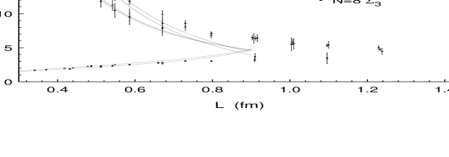
Figure 12: Numerical data [80] for the SU(2) electric flux energies, $E_{e_{n}}=L\Sigma_{n}\sqrt{n}$, with twisted boundary conditions, ${\bf m}=(1,1,1)$, on lattices of size $N^{3}\times N_{t}$, with $N=4,6,8$ and resp. $N_{t}=128,128,64$. The scale is set by $L=400N\exp(-3.38\beta)\,{\rm fm}$ and the curves show the perturbative predictions combined with a fit to the expected tunneling contributions.

Also an extensive study was made of the electric flux energies.[79, 80] Here lattices of size $8^{3}\times 64$ and $N^{3}\times 128$ with $N=4$, 6 were used, with $\beta=4/g_{0}^{2}$ ranging from 2.25 to 2.6, reaching volumes between 0.3 and 1.3 fermi. In Fig. 12 $\Sigma_{n}=E_{e_{n}}/(L\sqrt{n})$ is plotted as a function of $L$. This definition is such that if, as predicted by ’t Hooft,[9] $R_{n}\rightarrow\sqrt{n}$ in the infinite volume limit, $\Sigma_{n}$ gives the infinite volume string tension $K$ independent of $n$. The curves test the small volume expansion. They contain the perturbative contribution, corrected for the lattice artifacts [75] (the data is not accurate enough to test the $\mbox{$\cal O$}\left(g_{0}^{2}\right)$ corrections), together with const.$\times g_{0}^{-4}\exp(-S/g_{0}^{2})$, the expected shift due to tunneling (cmp. Fig. 11 and Sec. 6.4) mediated by the charge ${\scriptstyle{{1\over 2}}}$ instanton with classical action $S$ ($4\pi^{2}$ in the continuum, see Sec. 4). The constant is fitted separately for $N=4$ and 6 ($N=8$ fits not shown). One finds fair agreement with the predicted behavior, with confirmation that the transition to the large volume starts around 0.75 fermi.

3.5 Supersymmetry and the Witten Index

The case of supersymmetric Yang-Mills theories in a finite volume has been considered in the context of the Witten index [10] in some detail. The torus geometry is crucial to preserve the gauge invariance. The Witten index involves counting the number of quantum states (fermionic states with a negative sign). At non-zero energy, because of the supersymmetry, this number cancels between the bosonic and fermionic states, such that the counting can be reduced to the vacuum sector. Here the number can be non-zero, because the supersymmetry generator can annihilate vacuum states. A zero Witten index is a sign of spontaneous breakdown of supersymmetry, where the vacuum energy is non-zero, explaining the physical significance of this index. A zero vacuum energy is a direct consequence of unbroken supersymmetry, where the hamiltonian is given by $H={\scriptstyle{{1\over 2}}}\{Q,Q^{\dagger}\}$ with $Q$, $Q^{\dagger}$ the supersymmetry generators, that annihilate the vacuum state.

In perturbation theory bosonic loops are typically cancelled by fermionic loops, e.g. in the vacuum energy. Applied to the problem of non-abelian gauge theories in a finite volume this implies that the vacuum-valley effective potential vanishes. The cancellation is caused by the contribution from the gluino fluctuations, which are the superpartners of the gluons. They are Weyl fermions in the adjoint representation of the gauge group, denoted by $\lambda_{\alpha}^{a}$, with $\alpha$ a two-component spinor index. This means that the wave function is no longer localized to $A=0$ or any of the other orbifold singularities of the vacuum valley (the moduli space of flat connections). It has been shown in the context of the supermembrane, when taking the supersymmetric Yang-Mills hamiltonian restricted to the zero-momentum modes only, that the spectrum is continuous, down to zero-energy. One can construct trial wave functions with a support arbitrarily far from $A=0$ that nevertheless have finite energy.[93] The compactness of the vacuum valley is crucial to obtain a discrete spectrum.

The counting of quantum vacuum states was based on the assumption that for all gauge groups the moduli space of flat connections is given in terms of the Cartan subalgebra, as we discussed for SU($N$). The gluonic part of the groundstate wave function $|0\rangle$ is assumed to be constant over the vacuum valley. In the reduction to the vacuum valley there are $r$ gluinos (associated with the generators in the Cartan subalgebra), each with two helicities. They are constant and carry no energy, which is the source of the vacuum degeneracy. These gluinos have to be combined in Weyl invariant combinations, respecting Fermi-Dirac statistics. There are $r$ independent invariants, made from

$$U=\delta_{ab}\epsilon^{\alpha\beta}\lambda_{\alpha}^{a}\lambda_{\beta}^{b}$$ (45)

and its powers. So one has $U^{n}|0\rangle$, $n=0,1,\cdots,r$, as the $r+1$ bosonic vacuum states, with no invariant fermionic vacuum states. Thus, one finds an index equal to the rank of gauge group plus one, $r+1$.

Because of possible problems with the adiabatic approximation near the orbifold singularities, as we encountered in the previous sections, Witten considered the alternative of twisted boundary conditions.[10] For SU($N$) the same result, $r+1=N$, for the index follows. Other groups in general do not admit the type of twisted boundary conditions that completely remove the continuous vacuum degeneracy with its orbifold singularities. So it was natural to attempt to find the exact zero-energy ground state for the supersymmetric generalization of Lüscher’s zero-momentum effective hamiltonian,[94] or even ignoring the time dependence, studying the path integral in the ultra local limit.[95] None of these studies took the compactness of the vacuum valley into account and therefore fail to address the proper situation.[93]

The problem of the adiabatic approximation remained an urgent one because of a discrepancy between the finite volume calculation of the Witten index, and the one based on the infinite volume determination of the gluino condensate through instanton contributions.[96, 97, 99] One relies on the fact that an index can not change under smooth perturbations, like increasing the volume. Also the infinite volume calculation has its problems. It uses the semiclassical approximation for a strongly interacting theory. This could, however, be circumvented by first adding matter fields to introduce an external mass scale to control the instanton calculation and then rely on the index being constant under a smooth deformation (through holomorphy), that decouples the extra matter sector.[97] This resulted nevertheless in a discrepancy, $\sqrt{5/4}$ for SU(2), between the so-called strong and weak coupling calculations. Both calculations rely on the cluster decomposition property, since the instantons have more than two gluino zero modes, which seems to make the condensate $\langle\lambda\lambda\rangle$ vanish. The instanton calculation instead computes the appropriate power of the gluino condensate, $\langle(\lambda\lambda)^{h}\rangle$, that saturates the $2h$ gluino zero modes, where $h$ is the so-called dual Coxeter number of the gauge group, $h=N$ for SU($N$). It is this power that gives the number of vacuum states,

$$\langle\lambda\lambda\rangle\equiv e^{2\pi in/h}\left(|\langle(\lambda\lambda)^{h}\rangle|\right)^{1/h},\quad n=1,2,\cdots,h.$$ (46)

These arguments seem reasonable, but are not rigorous.[99] See for further details a review by Shifman.[98] Recently, use has been made of the constituent nature of periodic instantons (or calorons),[100, 101] in the context of a Kaluza-Klein reduction with periodic gluinos, as opposed to a high temperature reduction with anti-periodic gluinos, which would break the supersymmetry. The constituent monopoles have exactly two zero-modes and saturate the condensate, $\langle\lambda\lambda\rangle$. The strong coupling calculation now agrees with the weak coupling result.[102] The period can of course be used to control the coupling constant, but it is assumed the index does not change, going from a small to a large period.

The mismatch in the Witten index between small and infinite volumes occurs for SO($N>6$) and the exceptional groups. There has, however, been a recent revision in counting the number of vacuum states in a finite volume. In a study of D-brane orientifolds in string theory, Witten [103] constructed for SO(7) an extra disconnected component on the moduli space of flat gauge connections, which can be embedded easily in SO($N>7$). For SO(7) and SO(8) this gives an isolated component of the moduli space, contributing only one extra vacuum state. For SO($N>8$) the extra component in the moduli space behaves like the trivial component for SO($N$-7). Adding $r+1$ coming from the SO($N$) and SO($N-7$) moduli space components gives the dual Coxeter number of SO($N$), thereby giving the same number of vacuum states as obtained in the infinite volume.

Witten’s construction based on orientifolds does not work for the exceptional groups. This naturally led to a derivation of the extra vacuum states in a field theoretic context,[104] trivially extended to the exceptional group $G_{2}$, as a subgroup of SO(7). Three different groups have independently managed to solve the problem for other exceptional groups with periodic boundary conditions [105, 106] and for any group with twisted boundary conditions.[107] As we remarked before, twisted boundary conditions usually do not remove all the vacuum degeneracies, but it is important that the number of vacuum states is independent of the twist for all gauge groups that have a non-trivial center. The origin of the extra moduli space components is actually not too hard to understand.[105] Large gauge groups can have subgroups that are products of unitary groups, which each would allow for twisted boundary conditions. By choosing twists from all subgroups to cancel one obtains periodic flat connections that can not be deformed to the Cartan subalgebra, which supports the trivial component of flat connections. Of course one need not cancel these twists completely.[107] Needless to say, the group theory involved to sort out all the constraints and count the number of vacuum components is rather involved.

Supersymmetry does not play a role in establishing the existence of these extra vacuum components. Supersymmetry is, however, crucial for these extra components to lead to extra quantum vacua. As soon as the perturbative quantum fluctuations in the vacuum energy do not cancel, this will in general be different for different vacuum components. In a small volume, i.e. at weak coupling, the wave functional will localize around the one with the lowest vacuum energy. Within such a connected component it will localize around the minimum of the effective potential, as we discussed in the previous sections. It is likely, since the trivial vacuum component is the widest, that this is the one where the wave functional localizes. But interestingly, one now has potential energy barriers between vacuum components that are not related by a homotopically non-trivial gauge transformation (since the different vacuum components are not isomorphic). Still these vacua can be characterized by fractional Chern-Simons numbers and tunneling between them would be described by new types of instanton solutions with fractional topological charge.[107, 105] It considerably adds to the richness of non-abelian gauge theories.

Although these new results for counting the number of vacuum states in a finite volume remove the urgency of addressing the problem with the adiabatic approximation, it does remain a sore point in the finite volume analysis, as also stressed recently by Witten.[108] One immediate problem we encounter is that Eq. (22) seems to imply that the vacuum-valley wave function has to vanish at the orbifold singularities, which seems inconsistent with it being constant sufficiently far from the orbifold singularities. However, one should take into account the behavior under Weyl reflections of the occupied negative energy gluino states in the Dirac sea near the orbifold singularities in the zero-momentum hamiltonian. Attempting to incorporate this in the formalism developed in the previous sections, we run into the problem that spin ${\scriptstyle{{1\over 2}}}$ fields do not decompose in three components, which can be associated with each of the coordinate directions. In the bosonic sector we could conveniently ignore the transversality, with gauge invariance restored at the end by restricting to the invariant wave functions. Thereby each of the coordinate directions separately allowed a polar decomposition, not compatible with the nature of the gluino fields. For SU(2) there is, however, an elegant polar decomposition using the spherical and gauge symmetry of the zero-momentum hamiltonian,[109] which even holds for $H_{{\rm eff}}$ in Eq. (3) to $\mbox{$\cal O$}\left(g^{4/3}\right)$. In the supersymmetric case one would require the wave function to become constant after reduction to the vacuum valley, sufficiently far away from $A=0$, to match to the expected behavior away from each of the orbifold singularities. Such a matching can in principle be controlled sufficiently rigorously,[28] as was done in the semiclassical calculation of the energy of electric flux,[29, 30] but here we do not have the benefit of a well localized zero-momentum wave function at the orbifold singularities,[93] and judging the incomplete results in the literature,[94] this seems not the way to go. It is in the light of the robustness of supersymmetry somewhat surprising (and frustrating) this problem remains so technically demanding.

4 Instantons and Sphalerons on the Torus

Instantons are associated with the tunneling through barriers that separate different vacuum components. We are interested in these barriers to establish the directions in field space in which the spreading of the wave functional has to be taken into account, when energies of the low-lying states no longer are well below the barriers. The barrier is a saddle point of the energy functional with one unstable mode, a so-called sphaleron.[81] They exist here by virtue of the finite volume. Remarkably, on any compact four manifold instantons exist,[82, 83] still with an arbitrary scale parameter, only limited by the size of the manifold. The finite volume sphaleron is typically associated with the instanton that achieves this maximal scale.

For low topological charge, sometimes smooth instantons can not be proven to exist.[82] An example of non-existence actually occurs [84] on $T^{\,4}$. In general one takes a small localized instanton from ${\rm I\kern-1.79993ptR}^{4}$ that is matched smoothly to the flat connection. When the moduli space of flat connections has a continuous degeneracy, as is the case for the torus, there can be obstructions against this procedure. One can get arbitrarily close to satisfying the self-duality equations, $F_{\mu\nu}=\pm\tilde{F}_{\mu\nu}\equiv\pm{\scriptstyle{{1\over 2}}}\epsilon_{\mu\nu\alpha\beta}F^{\alpha\beta}$, that saturate the bound for the euclidean action

$$S=-{\scriptstyle{{1\over 2}}}\int\mbox{\,tr\,}(F_{\mu\nu}^{\,2})=-{\scriptstyle{{1\over 4}}}\int\mbox{\,tr\,}(F_{\mu\nu}\pm\tilde{F}_{\mu\nu})^{2}\pm{\scriptstyle{{1\over 2}}}\int\mbox{\,tr\,}(F_{\mu\nu}\tilde{F}^{\mu\nu})\leq 8\pi^{2}|\nu|,$$ (47)

with $\nu$ the topological charge. However, an exact self-dual solution is only achieved in the limit where the scale parameter is forced to zero or the volume is taken to infinity. For twisted boundary conditions [9], existence of charge one instantons [85] can be understood from the fact that twist removes the continuous degeneracy in the moduli space of flat connections.

From the hamiltonian point of view we are interested in instantons on $T^{3}\times{\rm I\kern-1.79993ptR}$, where time is not constrained to be finite. This can be seen as a limit of $T^{\,4}$ where one of the periods, called $T$, is taken to infinity. In the $A_{0}=0$ gauge the field is periodic up to a gauge transformation $h$ in the time direction, $A({\bf x},T)=[h]A({\bf x},0)$, and

$$-\frac{1}{16\pi^{2}}\int\mbox{\,tr\,}(F_{\mu\nu}\tilde{F}^{\mu\nu})=\int_{0}^{T}CS(A)=CS([h]A)-CS(A)=\nu(h),$$ (48)

with $\nu(h)$ defined in Eq. (15). Using that $\mbox{\,tr\,}(F_{\mu\nu}\tilde{F}^{\mu\nu})=\partial_{\mu}K_{\mu}(A)$, we find for the Chern-Simons functional

$$CS(A)=-\frac{1}{16\pi^{2}}\int d^{3}xK_{0}(A)=-\frac{1}{8\pi^{2}}\int d^{3}x\mbox{\,tr\,}\left(A_{i}(\partial_{j}A_{k}+{\scriptstyle{{2\over 3}}}A_{j}A_{k})\right)\epsilon_{ijk}.$$ (49)

When $T^{3}$ has periodic boundary conditions there is an ambiguity which point in the vacuum valley to tunnel from and to. These need not be the same points, as is already evident with tunneling related by non-trivial twisted gauge transfomations (see Eq. (20) and (35)), under which the Polyakov loop is periodic in time up to a non-trivial $Z_{N}$ factor. In that case charge one instanton solutions can be shown to exist.[85] The obstruction for the periodic four-torus is reflected in the fact that the instanton does not want to tunnel between the same points in the vacuum valley.

Figure 13: Numerical results [87] obtained with cooling on $N^{3}\times 3N$ lattices (scaled to $L=1$). Left is with ${\bf k}={\bf 0}$, $N=8$ and right with ${\bf k}=(1,1,1)$, $N=7$ and 8 (${\bf k}$ indicating the twist in time). The top figures show electric ($\mbox{$\cal E$}_{E}(t)$ triangles) and magnetic ($\mbox{$\cal E$}_{B}(t)$ squares) energies ($g=1$), the inset shows the tails at an enlarged scale. In the lower figures we plot $C_{2}(t)$ through two distinct (on the right one) point(s).

This is illustrated in Fig. 13, obtained by a numerical procedure called cooling [86] that minimizes the lattice action in a given topological sector, carefully dealing with the lattice discretization problems.[87] With periodic boundary conditions the configuration first relaxes to a solution which is not self-dual, although it has reached the vacuum valleys at either end in euclidean time, judging the zero magnetic energy. However, it moves in accordance with the equations of motion along this vacuum valley with constant speed (i.e. electric field) to match the forced periodicity, as is also evident from the linear (space independent) slope for $C_{2}(t)$. When one would continue to lower the action, in order to reach a self-dual solution, the instanton is forced to shrink to zero size. With a twist in the time direction the configuration immediately relaxes to a self-dual one.

Table 2: The lowest eigenvalues [33] for the Hessian of the energy functional evaluated at the twisted and periodic sphaleron on a $N^{3}$ lattice for $N=4,~{}6$ and 8.

m=(1,1,1)  sphaleron${\vphantom{|}}^{\vphantom{|}}$			m=0  sphaleron${\vphantom{|}}^{\vphantom{|}}$
N=4	N=6	N=8	N=4	N=6	N=8
-11.1280	-10.9003	-10.8174	-13.1960	-13.3935	-13.4432
0.0074	0.0001	0.0000	0.0073	0.0006	0.0000
0.0091	0.0001	0.0000	0.0124	0.0010	0.0000
0.0101	0.0001	0.0000	0.0139	0.0011	0.0000
13.1667	13.3371	13.3934	1.7041	1.4151	1.3009
13.1667	13.3371	13.3934	1.7070	1.4303	1.3012
13.1667	13.3372	13.3934	7.9677	8.0984	8.1260
16.0475	16.8663	17.1597	7.9682	8.1008	8.1261
16.0478	16.8663	17.1597	7.9684	8.1279	${\vphantom{|}}_{\vphantom{|}}$ 8.1266

Shown on the right in Fig. 13 is an instanton that is close to being maximal in its size, thereby going through the lowest barrier, to maintain the same action. This lowest barrier is assumed to be a finite volume sphaleron. This was verified,[33] by explicitly looking for saddle-point solutions on $T^{3}$, minimizing the square of equations of motion using a similar numerical procedure of cooling (cmp. Fig. 14). This saddle point is not invariant under translations, giving rise to zero-modes, which in addition to the unstable (i.e. tunneling direction) will become the degrees of freedom that need to be treated non-perturbatively, by imposing the proper boundary conditions in field space. In addition it was found that there are two directions not associated with zero-modes, in which the saddle point is nearly flat (see Table 2). Such modes would have to be treated non-perturbatively as well. Without an analytic solution, it is hard to judge if such an analysis is feasible. This was one of the motivations to look at the situation where the torus geometry is replaced by that of a sphere. In this case the finite volume sphaleron has a constant energy density and no (almost) flat directions, see Sec. 5.

We already mentioned in the previous section that with non-zero magnetic flux, there exist instanton solutions with fractional topological charge. When first proposed by ’t Hooft,[73] this was met with some disbelieve. The mathematical classification of so-called fiber bundles, to describe gauge fields on compact manifolds seemed to require integer topological charge, specified by the second Chern number (see Eq. (54)). But due to the twist, the fiber bundle has to be considered real and the appropriate classification is by the first Pontryagin class. With the proper normalizations, this makes the would-be fractional second Chern class an integer first Pontryagin class.[50] It is the difference between a unitary and orthogonal fiber bundle, e.g. SU(2) versus SO(3). This makes also precise the intimate connection between the topological charge and twist, as first discovered by ’t Hooft.[73] As we have seen in Secs. 3.1 and 3.4 (see Eq. (35), which also applies for ${\bf m}={\bf 0}$, in which case $\Omega_{j}=1$), there are homotopically non-trivial gauge transformations $h_{{\bf k}}$, “periodic” up to an element of the center of the gauge group, that do not affect the boundary conditions of the gauge fields. In particular $h_{{\bf k}}^{-1}dh_{{\bf k}}$ has the right periodicity, and $\nu(h_{{\bf k}})$ in Eq. (15) remains well-defined (in the gauge where the twist matrices $\Omega_{j}$ are constant and $A_{0}=0$). When ${\bf m}={\bf 0}$ we have seen that we can always choose $h_{{\bf k}}$ abelian, and $\nu(h_{{\bf k}})=0$. In this case there is no interplay between the twist and the topological charge $\nu$, which is here integer. When ${\bf m}$ is non-trivial we stated in Sec. 3.4 that when ${\bf k}\cdot{\bf m}=0$ (mod $N$), $h_{{\bf k}}$ can be chosen constant, $h_{{\bf k}}=\Omega_{0}({\bf k})$, as can be checked for the simple case of SU(2) by inspection, but can be proven from first principles.[67] However, when ${\bf k}\cdot{\bf m}\neq 0$ mod $N$ it may be that $\nu(h_{{\bf k}})\neq 0$. The additive nature of the topological invariant $\nu(h)$,

$$\nu(h^{\prime}h)=\nu(h^{\prime})+\nu(h),$$ (50)

implies that $\nu(h_{{\bf k}}^{N})=N\nu(h_{{\bf k}})$. This has to be an integer, since $h_{{\bf k}}^{N}$ is “periodic” and the winding number of a periodic function $h:T^{3}\rightarrow G$ is an integer. Also one can duplicate $T^{3}$, under which the topological charge is additive, as many times in the space directions as is necessary to get a new torus for which ${\bf m}={\bf 0}$, and hence with integer topological charge. Therefore,[73] $\nu(h)$ is proportional to $N^{-1}$ and linear in ${\bf k}$ and ${\bf m}$, such that $\nu+{\bf m}\cdot{\bf k}/N\in{\rm Z\!\!Z}$, as was proven rigorously in the context of fiber bundles.[50] Conversely, using this result one easily sees that the existence of constant twist matrices in four dimensions, i.e. solutions to both Eq. (32) and Eq. (36), require ${\bf k}\cdot{\bf m}=0$ mod $N$. This is so because $A=0$, with $\nu=0$, satisfies the boundary conditions. For further details on these twist-related issues one can also consult a recent review.[88]

The above implies that the lowest non-trivial topological charge that can be reached is $1/N$. With Eq. (47), the associated euclidean action of this instanton solution is found to be $8\pi^{2}/N$, which can indeed be attained as one can prove existence of self-dual solutions in the appropriate sector.[89] Like for topological charge one, despite much effort up to date no analytic solutions are known. What can be deduced from general principles [90] is that the solutions with charge $1/N$ have only the four translational degrees of freedom. In particular they have no free scale parameter, their size is fixed with respect to the torus. This fixed scale is a great benefit in studying these instantons on the lattice.[91, 76, 92] For this fractionally charged instanton the finite volume sphaleron was constructed as well, by finding for SU(2) with twist ${\bf m}=(1,1,1)$ on $T^{3}$ the appropriate saddle point. Like for ${\bf m}={\bf 0}$ it is not invariant under translations, giving three flat directions at the saddle point, but in this case no other near zero-modes appear,[33] see Table. 2.

Figure 14: Numerical results [33] for $\tilde{S}(t)$, the square of the equations of motion, along the tunneling path for the SU(2), charge ${\scriptstyle{{1\over 2}}}$ twisted instanton solution for ${\bf m}={\bf k}=(1,1,1)$, evaluated on a $8^{3}\times 24$ (triangles) and a $12^{3}\times 36$ (squares) lattice (scaled to $L=1$). The dip at $t=0$ occurs at the finite volume sphaleron.

In Fig. 14 we illustrate the fact that along the tunneling path there is a saddle point, by plotting the square of the equations of motion,

$$\tilde{S}(t)\equiv-\frac{1}{32}\int_{T^{3}}d^{3}x\mbox{\,tr\,}\bigl{(}\partial_{i}F_{ij}({\bf x})+[A_{i}({\bf x}),F_{ij}({\bf x})]\bigr{)}^{2},$$ (51)

as a function of euclidean time. The fact that $\tilde{S}$ does not exactly vanish in the middle, at the top of the barrier, is due to a limited resolution on the finite lattices employed.

4.1 T-duality for Instantons on the Torus

Although no explicit solutions of the basic instantons of charge $1/N$ and charge 1 are known, progress has been made in better understanding instantons on the torus. We will first discuss the case of $T^{4}$, before addressing $T^{3}\times{\rm I\kern-1.79993ptR}$. For $T^{4}$ the only explicitly known solutions are the ones constructed by ’t Hooft with constant field strength.[110, 111, 112] These are essentially abelian and are self-dual only when the periods of the torus match the field strength (which is quantized due to quantization of flux). Recently these solutions to the self-duality equations were followed in perturbation theory by deforming away from the special geometry,[113] using as a starting point the exact fluctuation spectrum [111] in the background of the non-selfdual constant curvature solutions.

The essential ingredient for gaining further understanding has been the so-called Nahm or Mukai transformation.[11, 114] Nahm introduced it to find magnetic monopole solutions, getting inspiration from the algebraic Atiyah-Drinfeld-Hitchin-Manin [115] (ADHM) construction of instantons in ${\rm I\kern-1.79993ptR}^{4}$. The formalism can as a matter of fact be used to provide a simple proof of the ADHM construction.[83, 116] It will be convenient in the following to see $T^{4}$ as ${\rm I\kern-1.79993ptR}^{4}/\Xi$, where $\Xi$ is a four dimensional lattice spanned by the four periods $a^{(\mu)}$, and to introduce the connection one-form $\omega(x)=A^{\mu}(x)dx_{\mu}$, which is invariant up to a gauge transformation under translation over a period. These gauge transformations, called cocycles, satisfy cocycle conditions [9] (twisted boundary conditions will be discussed later), to assure the gauge invariant quantities are periodic, and such that one has an appropriate fiber bundle over the torus,[50]

$$\omega(x+a) = h^{-1}_{a}(x)(\omega(x)+d)h_{a}(x),$$ (52)

$$h_{a+b}(x) = h_{b}(x)h_{a}(x+b)=h_{a}(x)h_{b}(x+a),\quad a,b\in\Xi.$$

It will be convenient to take U($N$) as gauge group, allowing for a U(1) factor. The associated vector bundle in the fundamental representation of U($N$) is denoted by $E$. The curvature of this bundle $E$, given by

$$F=d\omega+\omega\wedge\omega={\scriptstyle{{1\over 2}}}F^{\mu\nu}dx_{\mu}\wedge dx_{\nu},$$ (53)

leads to a topological charge $\nu=\int_{T^{4}}(c_{2}(E)-{\scriptstyle{{1\over 2}}}c_{1}(E)\wedge c_{1}(E))$ as an integral over Chern classes (cmp. Eq. (48) and note that $c_{1}(E)=0$ for SU($N$) because of the vanishing trace), where

$$c_{1}(E)=\mbox{\,tr\,}\left(\frac{F}{2\pi i}\right),\quad c_{2}(E)={\scriptstyle{{1\over 2}}}\mbox{\,tr\,}\left(\frac{F}{2\pi i}\wedge\frac{F}{2\pi i}\right).$$ (54)

The starting point of the Nahm transformation is that gauge fields with topological charge $\nu$, have $\nu$ positive chirality zero-modes for the massless Dirac equation,[117] which is most conveniently written in the Weyl representation. For this we introduce the unit quaternions $\sigma_{\mu}$ and their conjugates $\bar{\sigma}_{\mu}\equiv\sigma^{\dagger}_{\mu}$

$$\sigma_{\mu}=(1_{2},i\tau_{j}),\quad\bar{\sigma}_{\mu}=(1_{2},-i\tau_{j}).$$ (55)

They satisfy the multiplication rules

$$\sigma_{\mu}\bar{\sigma}_{\nu}=\eta^{\alpha}_{\mu\nu}\sigma_{\alpha},\quad\bar{\sigma}_{\mu}\sigma_{\nu}=\bar{\eta}^{\alpha}_{\mu\nu}\sigma_{\alpha},$$ (56)

where we used the ’t Hooft $\eta$ symbols,[22] generalized slightly to include $\eta^{0}_{\mu\nu}=\bar{\eta}^{0}_{\mu\nu}=\delta_{\mu\nu}$, also useful in Sec. 5. The Weyl-Dirac operator is given by

$$D\equiv\sigma_{\mu}D_{\mu}(A)=\sigma_{\mu}(\partial_{\mu}+A_{\mu}).$$ (57)

Hence, in the background of a charge $\nu$ gauge field there are $\nu$ independent solutions to $D\Psi=0$. For $\Psi(x)$ to be defined as a two-spinor on the torus one requires $\Psi(x+a)=h_{a}(x)\Psi(x)$. Strictly speaking, the index theorem [117] only states that the number of zero-modes of positive chirality minus those of negative chirality (for which $D^{\dagger}\Psi=0$) is equal to the topological charge, but it will be assumed that there are no negative chirality zero-modes. For self-dual gauge fields we will discuss this assumption later. One now adds a spectral parameter $z\in{\rm I\kern-1.79993ptR}^{4}$ in the form of a flat abelian connection [11]

$$\omega_{z}=\omega+2\pi iz^{\mu}dx_{\mu},$$ (58)

(the unit generator of U(1) is implicit) which leaves the curvature unchanged, $F_{z}=F$. Hence there is a smooth family of $\nu$ normalized fermionic zero-modes

$$D_{z}\Psi_{z}^{(i)}(x)=\sigma_{\mu}(\partial_{\mu}+A_{\mu}+2\pi iz_{\mu})\Psi_{z}^{(i)}(x)=0,\quad\int_{T^{4}}d^{4}x~{}\Psi_{z}^{(i)}(x)^{\dagger}\Psi_{z}^{(j)}(x)=\delta_{ij}.$$ (59)

From this family one constructs the connection $\hat{\omega}\equiv\hat{A}_{\mu}(z)dz_{\mu}$ by

$$\hat{A}_{\mu}^{ij}(z)=\int_{T^{4}}d^{4}x~{}\Psi_{z}^{i}(x)^{\dagger}\frac{\partial}{\partial z_{\mu}}\Psi_{z}^{(j)}(x).$$ (60)

Using that $D_{z+\hat{a}}\bigl{(}e^{-2\pi ix\cdot\hat{a}}\Psi_{z}^{(i)}(x)\bigr{)}=0$ and the fact that $\bigl{\{}\Psi_{z+\hat{a}}^{(i)}(x)\bigr{\}}$ forms a complete orthogonal set of solutions, we find that

$$\Psi_{z+\hat{a}}^{(i)}(x)=e^{-2\pi ix\cdot\hat{a}}\Psi_{z}^{(j)}(x)\hat{h}^{ji}_{\hat{a}}(z),$$ (61)

with $\hat{h}_{\hat{a}}(z)$ a unitary $\nu\times\nu$ matrix, which defines the cocycle for $\hat{\omega}$

$$\hat{\omega}(z+\hat{a})=\hat{h}^{-1}_{\hat{a}}(z)(\hat{\omega}(z)+\hat{d})\hat{h}_{\hat{a}}(z),\quad\hat{d}\equiv dz_{\mu}\partial_{z_{\mu}},$$ (62)

as a U($\nu$) connection on the dual torus $\hat{T}^{4}={\rm I\kern-1.79993ptR}^{4}/\tilde{\Xi}$, where

$$\tilde{\Xi}=\bigl{\{}\hat{a}\in{\rm I\kern-1.79993ptR}^{4}|<\hat{a},a>\in{\rm Z\!\!Z},\ \forall a\in\Xi\bigr{\}}$$ (63)

is the lattice dual to $\Xi$. For example, if $\Xi$ is generated by $a^{(\mu)}=Le^{(\mu)}$, giving a hypercube with sides of length $L$, the dual lattice $\tilde{\Xi}$ is generated by $\hat{a}^{(\mu)}=L^{-1}e^{(\mu)}$, a hypercube with sides of length $1/L$. So the Nahm transformation is a T-duality.

In the absence of negative chirality zero-modes ($\rm cokerD_{z}=\ker D_{z}^{\dagger}=0$) $\hat{E}_{z}\equiv\ker D_{z}$ depends smoothly on $z$. It was realized by Braam,[118, 119] that one can use the Atiyah-Singer family index theorem [117] to compute the Chern character of the bundle $\hat{E}$ with connection $\hat{\omega}$, as the integral over $T^{4}$ of the Chern character of $E\otimes\mbox{$\cal P$}$, which is the vector bundle relevant for $\omega_{z}$, as a vector bundle over $T^{4}\times\hat{T}^{4}$. Here $\cal P$ is the so-called [84] Poincaré line bundle with the connection $2\pi iz^{\mu}dx_{\mu}$. It was crucial this line bundle had no curvature as a bundle over $T^{4}$, but extending it to $T^{4}\times\hat{T}^{4}$, this is no longer the case and $F_{\mbox{$\cal P$}}=2\pi idx_{\mu}\wedge dz^{\mu}$, with a first Chern class, $c_{1}(\mbox{$\cal P$})=dx_{\mu}\wedge dz^{\mu}$ (for a line bundle all other Chern classes vanish). The Chern character satisfies $ch(E\otimes E^{\prime})=ch(E)\wedge ch(E^{\prime})$ and is a formal polynomial in the Chern classes,

$$ch(E)=c_{0}(E)+c_{1}(E)+{\scriptstyle{{1\over 2}}}c_{1}(E)\wedge c_{1}(E)-c_{2}(E),\quad ch(\mbox{$\cal P$})=\exp(c_{1}(\mbox{$\cal P$})).$$ (64)

Perhaps somewhat confusingly $c_{0}(E)=rk(E)$ is called the rank of the vector bundle $E$, here the dimension of the fundamental representation (so $rk(E)=N$ for a U($N$) fiber bundle). It now follows that

$$\rm ch(\hat{E})=\int_{T^{4}}\rm ch(E)\wedge\rm ch(\mbox{$\cal P$}).$$ (65)

The integral over $T^{4}$ only gives a non-zero result if the combined form is of degree four in $dx_{\mu}$, i.e. a top-form. This means that

• The zero-form $c_{0}(E)=N$, becomes a volume form on $\hat{T}^{4}$, whose integral over $\hat{T}^{4}$ gives the topological charge of the dual gauge field.

• The two-form $c_{1}(E)$ whose cohomology class can be specified by the abelian fluxes $c_{1}(E)={\scriptstyle{{1\over 2}}}n^{\mu\nu}dx_{\mu}\wedge dx_{\nu}$, goes over in $c_{1}(\hat{E})={\scriptstyle{{1\over 2}}}\tilde{n}^{\mu\nu}dz_{\mu}\wedge dz_{\nu}$.

• The four-form whose integral is the topological charge $\nu$ of the original gauge field becomes a zero-form, $c_{0}(\hat{E})=\nu$.

Thus we see that the Nahm transformation interchanges the rank $N$ of the bundle with the topological charge $\nu$, and maps the first Chern class to its dual. In particular, an SU($N$) bundle has vanishing first Chern class and is thus mapped under the Nahm transformation to U($\nu$) with vanishing first Chern class. It is well-known that in the latter case the bundle can be gauged to an SU($\nu$) bundle (its U(1) part is trivial and can be gauged away).

The family index theorem only provides topological information on the dual gauge field. We will demonstrate the wondrous result [11], that if $\omega$ is a self-dual connection, than also $\hat{\omega}$ is self-dual. A crucial ingredient is formed by

$$D^{\vphantom{\dagger}}_{z}D^{\dagger}_{z}=-D^{2}_{\mu}(A_{z})-{\scriptstyle{{1\over 2}}}\sigma_{[\mu}\bar{\sigma}_{\nu]}F^{\mu\nu},$$ (66)

using $\sigma_{\mu}\bar{\sigma}_{\nu}=\delta_{\mu\nu}+\sigma_{[\mu}\bar{\sigma}_{\nu]}$. Since $\sigma_{[\mu}\bar{\sigma}_{\nu]}\equiv\sigma_{i}\eta^{i}_{\mu\nu}$ is an anti-selfdual tensor, we see that $D^{\vphantom{\dagger}}_{z}D^{\dagger}_{z}=-D^{2}_{\mu}(A_{z})$. We first deal as promised with the condition that there are no opposite chirality zero-modes. We have seen that if $\omega$ is self-dual, and $D_{z}^{\dagger}\Psi=0$ that $D_{\mu}^{2}(A_{z})\Psi=D^{\vphantom{\dagger}}_{z}D_{z}^{\dagger}\Psi=0$, but this would imply that the connection $\omega$ has a flat factor, [83] meaning that the bundle of rank $N$ splits in the direct sum of a bundle of rank $N-1$ and a flat line bundle, $E=E^{\prime}\oplus L_{\xi}$, where $L_{\xi}$ has the connection $2\pi\xi^{\mu}dx_{\mu}$. Such a flat factor would exist for any $z$ (simply shifting $\xi$ proportionally), and so a sufficient condition to impose the absence of opposite chirality zero-modes is to require $\omega$ to be without flat factors (WFF, sometimes also called 1-irreducible).

A direct corollary is now that regular SU($N$) charge one instantons cannot exist on $T^{4}$. Suppose they would exist. The Nahm transformation gives rise to a U(1) bundle of charge $N$, which is impossible as the first Chern class vanishes and U(1) bundles have always vanishing second Chern class. Suppose flat factors prevent us from making the argument. In that case we can remove the flat factor and go down in rank by one (which keeps the first Chern class zero). This can be repeated until we are left with an SU($N-k$) charge one instanton without flat factors, or completely reduce to flat factors which, however, can not support topological charge.

Assuming no flat factors for the self-dual connection $\omega$, the kernel of $D^{\vphantom{\dagger}}_{z}D^{\dagger}_{z}$ is trivial and the well-defined Greens function $G_{z}=(D_{z}^{\vphantom{\dagger}}D_{z}^{\dagger})^{-1}$ commutes with the quaternions $\sigma_{\mu}$. It is now straightforward to show that $\hat{\omega}$ is self-dual as well

$$\hat{F}^{ij}(z)=\hat{d}\hat{\omega}^{ij}+\hat{\omega}^{ik}\wedge\hat{\omega}^{kj}=<\hat{d}\Psi_{z}^{(i)}|1-P_{z}|\hat{d}\Psi^{(j)}_{z}>,$$ (67)

where $P_{z}$ is the projection on $\ker D_{z}$,

$$P_{z}\equiv\sum_{k=1}^{\nu}|\Psi_{z}^{(k)}><\Psi_{z}^{(k)}|=1-D_{z}^{\dagger}G_{z}D_{z}^{\vphantom{\dagger}}.$$ (68)

The equality to the right-hand side is trivially true for a zero-mode, whereas the orthogonal complement of $\ker D_{z}$ is described by the image of $D_{z}$, on which both sides act as the identity. Next we use $D_{z}\hat{d}\Psi_{z}^{(i)}=[D_{z},\hat{d}]\Psi_{z}^{(i)}=-2\pi idz_{\mu}\sigma^{\mu}\Psi_{z}^{(i)}$ to find

$$\hat{F}_{\mu\nu}^{ij}(z)=8\pi^{2}<\Psi^{(i)}_{z}|\bar{\sigma}_{[\mu}\sigma_{\nu]}G_{z}|\Psi_{z}^{(j)}>.$$ (69)

Self-duality immediately follows from the fact that $\bar{\sigma}_{[\mu}\sigma_{\nu]}=\sigma_{i}\bar{\eta}^{i}_{\mu\nu}$ is self-dual.

For $T^{4}$, applying the Nahm transformation the second time, it can be shown that $\omega$ is retrieved identically, and the explicit form of $\hat{\Psi}_{x}(z)$ in terms of $\Psi_{z}(x)$ allows one to show that metric and hyperKähler structures of the moduli spaces are preserved under the Nahm transformation. In other words, if we denote by $\mbox{$\cal M$}_{N,\nu}$ the moduli space of SU($N$) charge $\nu$ instantons, the Nahm transformation induces a map between moduli spaces, $\mbox{$\cal N$}:\mbox{$\cal M$}_{N,\nu}\rightarrow\mbox{$\cal M$}_{\nu,N}$, which is an involution that preserves the natural metric and hyperKähler structure of the moduli space.[84] The dimension of the moduli space, $4N\nu$, is indeed symmetric under interchanging $\nu$ and $N$.

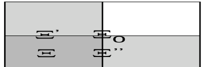
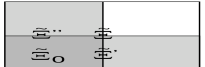
Figure 15: Shown is a cross section through the 1-2 plane of the various unit cells that appear in the Nahm transformation for SU(2) with twisted boundary conditions $n_{12}=-n_{21}=1$ on $R^{4}/\Xi$. We have chosen here $||a^{(1)}||=||a^{(2)}||={\scriptstyle{{1\over 2}}}\sqrt{2}$. Duplicated unit cells without twist are $\Xi^{\prime}$ and $\Xi^{\prime\prime}$, their union is denoted by $\Xi_{0}$. Its dual, $\tilde{\Xi}_{0}$, gives the torus on which the Nahm transformed gauge field lives, with the same gauge group and twist as for the gauge field we started with. The unit cell $\tilde{\Xi}_{0}$ is also obtained by intersecting $\tilde{\Xi}^{\prime}$ and $\tilde{\Xi}^{\prime\prime}$, the duals of the duplicated unit cells. When a symbol overlaps with different cells it belongs to all of those cells as a whole.

The Nahm transformation on $T^{4}$ can be defined to include twisted boundary conditions, as González-Arroyo has shown recently.[120] The basic idea is simple: One duplicates the unit cell, also denoted by $\Xi$, in the various directions as many times as is necessary to remove the twist. Let us assume for SU(2) $n_{12}=-n_{21}=m_{3}=1$ and the rest of the twist factors trivial. We can duplicate $\Xi$ either in the 1- or in the 2-direction in order to remove the twist, giving $\Xi^{\prime}$ and $\Xi^{\prime\prime}$. In both cases we can apply the Nahm to the enlarged unit cells $\Xi^{\prime}$ or $\Xi^{\prime\prime}$, see Fig. 15. In each case its dual $\tilde{\Xi}^{\prime}$ or $\tilde{\Xi}^{\prime\prime}$ is shorter by a factor 2 in the direction we originally duplicated. These two choices of unit cell intersect in a cell we call $\tilde{\Xi}_{0}$ that is twice shorter in each of the two directions. Due to the intersection it contains all the gauge invariant information of $\hat{\omega}^{\prime}$ and $\hat{\omega}^{\prime\prime}$. The gauge field therefore has half-periods associated with twisted boundary conditions on ${\rm I\kern-1.79993ptR}^{4}/\tilde{\Xi}_{0}$. In this particular example the resulting twist is the same as we started with. The argument can be generalized, either along the above lines, or using so-called flavor multiplication,[120, 121] to arbitrary SU($N$) and twist. The example shown in Fig. 15 (with identical behavior in the 0-3 plane), maps the charge ${\scriptstyle{{1\over 2}}}$ instanton to the same solution. Another example of self-similarity occurs for SU(2) in the charge 2 sector. When applied to the special solutions of ’t Hooft,[110] this can be used as an example where the Nahm transformation can be worked through analytically. The resulting Nahm transformed connection is again of the special form.[122]

To have the Nahm transformation help us finding explicit instanton solutions, simplifications have to be arranged for. These happen to be perfectly geared to finding charge one instanton solution on $T^{3}\times{\rm I\kern-1.79993ptR}$. For charge one the Nahm transformed gauge field is abelian and with one period infinite, the dual period collapses to zero. The decompactification limit $T\rightarrow\infty$ is associated with dimensional reduction. This reaches a dramatic height for the case that all periods are send to infinity, relevant for instantons on ${\rm I\kern-1.79993ptR}^{4}$. The dual is now a single point, explaining why the ADHM construction [115] is in essence algebraic. However, under the decompactification limit, a partial integration is required in going from Eq. (67) to Eq. (69),

$$\hat{F}_{\mu\nu}^{ij}(z) = 4\pi i\bar{\eta}^{k}_{\lambda\,[\mu}\oint d^{3}_{\lambda}x~{}\frac{\partial}{\partial z_{\nu]}}\left(\Psi^{(i)}_{z}\right)^{\dagger}\!(x)~{}\sigma_{k}\left(G_{z}\Psi_{z}^{(j)}\right)(x)$$ (70)

$$+8\pi^{2}\bar{\eta}^{k}_{\mu\nu}<\Psi^{(i)}_{z}|\sigma_{k}G_{z}|\Psi_{z}^{(j)}>.$$

These boundary terms destroy self-duality of $\hat{F}$, which can be repaired [11, 116] for instantons on ${\rm I\kern-1.79993ptR}^{4}$ and for calorons (periodic instantons) on ${\rm I\kern-1.79993ptR}^{3}\times S_{1}$. Except for ${\rm I\kern-1.79993ptR}^{4}$, for which there is no freedom, the location of the singularities are fixed by the asymptotically flat connections at $t\rightarrow\pm\infty$, which are required to occur to keep the action finite. The Weyl-Dirac hamiltonian in the background of a flat connection has generically a mass gap. The mass gap vanishes, however, in particular when the flat connection is pure gauge. The flat connections are characterized by ${\bf A}_{z}=2\pi i~{}{\rm diag}\bigl{(}{\bf w}^{(1)}+{\bf z},\cdots,{\bf w}^{(N)}+{\bf z}\bigr{)}$, and for the mass gap to vanish it is sufficient that $||{\bf w}^{(k)}+{\bf z}||=0$ for any of the $N$ values of $k$. With two asymptotically flat connections, their are $2N$ corresponding values of ${\bf z}$ (which are defined modulo $\tilde{\Xi}$) where the mass gap vanishes. Only here the boundary terms in Eq. (70) can be non-vanishing. A simple steepest descent analysis in their neighborhood shows that they act as point sources with abelian electric and magnetic charges $\pm\pi$, enforced by charge quantization (positive charges associated with the flat connection at $t=\infty$). This ensures the magnetic sources are Dirac monopoles with unobservable Dirac strings.[123] Outside of the singularities the abelian field is self-dual and, noting the $z_{0}$ independence, $\hat{B}_{j}({\bf z})=\hat{E}_{j}({\bf z})=-\partial\hat{A}_{0}({\bf z})/\partial z_{j}$, where

$$\hat{A}_{0}({\bf z})=\frac{i}{2}\sum_{j=1}^{N}\sum_{{\bf n}\in\tilde{\Xi}}\left(||{\bf w}_{+}^{(j)}+{\bf z}+{\bf n}||^{-1}-||{\bf w}_{-}^{(j)}+{\bf z}+{\bf n}||^{-1}\right).$$ (71)

For the usual normalization of abelian fields one multiplies this with $-i$. The sum over the periods $\tilde{\Xi}$ on $\hat{T}^{3}$, although formally divergent, can be resummed in a rapidly converging series and one has an exact result [123] for $\hat{A}_{0}({\bf z})$ (see Fig. 16).

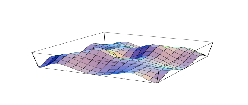
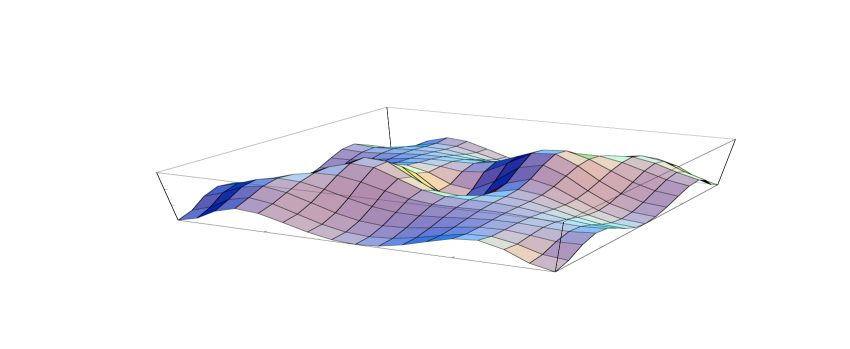
Figure 16: Comparison [121] of $\hat{\bf E}^{2}$ in the plane $z_{3}=0.5$ for the Nahm transformation of an SU(2) instanton on an $8^{3}\times 40$ lattice (scaled to $L=1$) and twist ${\bf k}=(1,1,1)$ in the time direction (left), with the analytic result on $T^{3}\times{\rm I\kern-1.79993ptR}$ for $P_{j}^{-}=(0.86,0.76,0.08)=-P_{j}^{+}$ (right).

One may argue from this that indeed time-periodic instanton solutions do not exist, as for ${\bf w}_{+}^{(j)}={\bf w}_{-}^{(j)}$ we clearly find $\hat{A}_{0}({\bf z})=0$, which under the Nahm transformation leads to a trivial connection on $T^{3}\times{\rm I\kern-1.79993ptR}$. With twisted boundary conditions in the time direction one has ${\bf w}_{+}^{(j)}={\bf w}_{-}^{(j)}+{\bf k}/N$. Although it is not straightforward to solve the Weyl-Dirac equation on $\hat{T}^{3}$ in the background of an abelian self-dual gauge field generated by point charges, one may hope explicit solutions of charge one instantons on the torus can be found this way.

The situation with the twisted instantons of fractional charge is, perhaps somewhat paradoxically, a bit more complicated. However, much understanding has been gained through the numerical implementation of the Nahm transformation on a lattice.[124] It has been found [121] that, in staying away from the exact decompactification limit, the Dirac monopole singularities are resolved into the fully non-abelian constituent monopoles that appear in the calorons, [100] with the only difference that these calorons are now modified by the finite volume,[125] for which no exact analytic solutions are available. They nevertheless fit very well to the infinite volume solutions, whereas away from the non-abelian cores of the constituent monopoles there is a nearly perfect fit to the abelian field of the singular Dirac monopoles. This aspect is illustrated in Fig. 16, comparing the analytic result in the decompactification limit with the numerical result on a lattice. For further details one should consult the literature.[121] It is natural to conjecture, in the light of these results that the fractionally charged instanton is mapped to a single point charge on a torus with (abelian) C periodic boundary conditions [57] in the decompactification limit.

5 Gauge Fields on the three-Sphere

The most important reason to study gauge fields on the three-sphere is that conformal equivalence of $S^{3}\times{\rm I\kern-1.79993ptR}$ to ${\rm I\kern-1.79993ptR}^{4}$ gives a very simple and explicit construction for the instantons.[126, 127] This allows one to formulate in a precise way how the $\theta$ dependence can be encoded in the boundary conditions on the fundamental domain.[126, 128] Due to the curvature of the sphere, at large volumes the corrections to the glueball masses are in powers of the inverse radius, as opposed to an exponential approach for the torus (to be discussed in Sec. 6.1). But ultimately, any geometry can be scaled-up to an infinite volume, and should in this limit give the same results. Therefore, by comparing different geometries we may indirectly get some useful information.

We embed $S^{3}$ in ${\rm I\kern-1.79993ptR}^{4}$ by considering the unit sphere (the radius $R$ can be reinstated on dimensional grounds where required), parametrized by a unit vector $n_{\mu}$. Alternative formulations, useful for diagonalizing the Faddeev-Popov and fluctuation operators, were developed by Cutkosky. [129] We can use the ’t Hooft tensors $\eta$ and $\bar{\eta}$ to define orthonormal framings [130] of $S^{3}$, which were motivated by the particularly simple form of the instanton vector potentials in these framings. The framing for $S^{3}$ is obtained from the framing of ${\rm I\kern-1.79993ptR}^{4}$ by restricting in the following equation the four-index $\alpha$ to a three-index $j$ (for $\alpha=0$ one obtains the normal on $S^{3}$, see Eq. (56)),

$$e^{\alpha}_{\mu}=\eta^{\alpha}_{\mu\nu}n_{\nu},\quad\bar{e}^{\alpha}_{\mu}=\bar{\eta}^{\alpha}_{\mu\nu}n_{\nu}.$$ (72)

Note that $e$ and $\bar{e}$ have opposite orientations. Each framing defines a differential operator with associated (mutually commuting) angular momentum operators ${\bf L}_{1}$ and ${\bf L}_{2}$:

$$\partial^{i}=e^{i}_{\mu}\frac{\partial}{\partial x^{\mu}},\quad L_{2}^{i}=\frac{i}{2}~{}\partial^{i}\quad,\quad\bar{\partial}^{i}=\bar{e}^{i}_{\mu}\frac{\partial}{\partial x^{\mu}},\quad L_{1}^{i}=\frac{i}{2}~{}\bar{\partial}^{i}.$$ (73)

It is easily seen that ${\bf L}_{1}^{2}={\bf L}_{2}^{2}$, which has eigenvalues $l(l+1)$, with $l=0,{\scriptstyle{{1\over 2}}},1,\cdots$.

By identifying the logarithm of the radius in ${\rm I\kern-1.79993ptR}^{4}$ as time in the geometry $S^{3}\times{\rm I\kern-1.79993ptR}$, the (anti-)instantons are easily obtained from those [21] on ${\rm I\kern-1.79993ptR}^{4}$

$$A_{0}=\frac{\varepsilon^{\mu}\cdot\sigma_{\mu}}{2(1+\varepsilon^{\mu}n_{\mu})},\quad A_{i}=\frac{\epsilon_{ijk}\sigma^{j}\varepsilon^{k}-(v+\varepsilon^{\mu}n_{\mu})\sigma_{i}}{2(1+\varepsilon^{\mu}n_{\mu})}.$$ (74)

Here $\varepsilon^{k}$, $\sigma_{j}$ and $A_{j}$ are defined with respect to the framing $\bar{e}^{j}_{\mu}$ for instantons and with respect to the framing $e^{j}_{\mu}$ for anti-instantons, and we introduced

$$u=\frac{2s^{2}}{1+b^{2}+s^{2}},\quad\varepsilon^{\mu}=\frac{2sb^{\mu}}{1+b^{2}+s^{2}},\quad s=\lambda\exp(t).$$ (75)

The unit quaternions $\sigma_{\mu}$ were given in Eq. (55). The instanton describes tunneling from $A=0$ at $t=-\infty$ to $A_{j}=-\sigma_{j}$ at $t=\infty$, over a potential barrier at $t=0$ that is lowest when $b\equiv 0$. This configuration corresponds to a sphaleron,[81] i.e. the vector potential $A_{j}=-{\scriptstyle{{1\over 2}}}\sigma_{j}$ is a saddle point of the energy functional with one unstable mode, corresponding to the direction ($u$) of tunneling. At $t=\infty$, $A_{j}=-\sigma_{j}$ has zero energy and is a gauge copy of $A_{j}=0$ by a gauge transformation $h=n_{\mu}\sigma^{\mu}$ with winding number one.

We will be concentrating our attention to the 18 modes that are degenerate in energy to lowest order with the modes that describe tunneling through the sphaleron and “anti-sphaleron”. The latter is a gauge copy by a gauge transformation $h^{\prime}=n_{\mu}\bar{\sigma}^{\mu}$ with winding number $-1$ of the sphaleron. The two dimensional space containing the tunneling paths through these sphalerons is consequently parametrized by $u$ and $v$ through

$$A_{\mu}(u,v)=\left(-u\bar{e}^{a}_{\mu}-ve^{a}_{\mu}\right)\frac{\sigma_{a}}{2}.$$ (76)

The gauge transformation $h$ with winding number one is easily seen to map $(u,v)=(w,0)$ into $(u,v)=(0,2-w)$. The 18 dimensional space is defined by

$$A_{\mu}(c,d)=\left(c^{a}_{j}\bar{e}^{j}_{\mu}+d^{a}_{j}e^{j}_{\mu}\right)\frac{\sigma_{a}}{2}=A_{j}(c,d)\bar{e}_{\mu}^{j}.$$ (77)

The $c$ and $d$ modes are mutually orthogonal and satisfy the Coulomb gauge condition, $\partial_{j}A_{j}(c,d)=0$. This space contains in it the $(u,v)$ plane through $c^{a}_{j}=-u\delta^{a}_{j}$ and $d^{a}_{j}=-v\delta^{a}_{j}$. The significance of this 18 dimensional space is that the energy functional [126]

$$\mbox{$\cal V$}(c,d) \equiv -\int_{S^{3}}\frac{1}{2}\mbox{\,tr\,}(F_{ij}^{\,2})=\mbox{$\cal V$}(c)+\mbox{$\cal V$}(d)+\frac{2\pi^{2}}{3}\left\{(c^{a}_{i})^{2}(d^{b}_{j})^{2}-(c^{a}_{i}d^{a}_{j})^{2}\right\},$$

$$\mbox{$\cal V$}(c) = 2\pi^{2}\left\{2(c^{a}_{i})^{2}+6\det c+\frac{1}{4}[(c^{a}_{i}c^{a}_{i})^{2}-(c^{a}_{i}c^{a}_{j})^{2}]\right\},$$ (78)

is degenerate to second order in $c$ and $d$. Indeed, the quadratic fluctuation operator $\cal M$ in the Coulomb gauge, defined by

$$-\int_{S^{3}}\frac{1}{2}\mbox{\,tr\,}(F_{ij}^{\,2}) = \int_{S^{3}}\mbox{\,tr\,}(A_{i}\mbox{$\cal M$}_{ij}A_{j})+\mbox{$\cal O$}\left(A^{3}\right),$$

$$\mbox{$\cal M$}_{ij} = 2{\bf L}_{1}^{2}\delta_{ij}+2\left({\bf L}_{1}+{\bf S}\right)^{2}_{ij},\quad S^{a}_{ij}=-i\epsilon_{aij},$$ (79)

has $A(c,d)$ as its eigenspace for the (lowest) eigenvalue $4$. These modes are consequently the equivalent of the zero-momentum modes on the torus, with the difference that their zero-point frequency does not vanish.

To find the fundamental region by minimizing the norm functional, Eq. (1), we can use $FP_{f}(A)$ in Eq. (6) as a hermitian operator acting on the vector space $\cal L$ of functions $h$ over $S^{3}$ with values in the space of the quaternions ${\rm I\!H}=\{q^{\mu}\sigma_{\mu}|q\in{\rm I\kern-1.79993ptR}^{4}\}$. The gauge group $\cal G$ is contained in $\cal L$ by restricting to the unit quaternions: $\mbox{$\cal G$}=\{h\in\mbox{$\cal L$}|h=h^{\mu}\sigma_{\mu},h\in{\rm I\kern-1.79993ptR}^{4},h_{\mu}h^{\mu}=1\}$. This allows us to extract detailed information about the Gribov and fundamental region within the 18 dimensional space $(c,d)$. When minimizing the norm functional over $\cal L$, instead of $\cal G$, one obviously should find a smaller space $\tilde{\Lambda}\subset\Lambda$. With $\cal L$ a linear space, $\tilde{\Lambda}$ can now also be defined by the condition that $FP_{f}(A)$ be positive,

$$\tilde{\Lambda}=\{A\in\Gamma|\left\langle h,FP_{f}(A)~{}h\right\rangle\geq 0,\ \forall h\in\mbox{$\cal L$}\}.$$ (80)

Similar to the Gribov horizon, the boundary of $\tilde{\Lambda}$ is now determined by the location where the lowest non-trivial eigenvalue of $FP_{f}(A)$ vanishes. For the $(c,d)$ space it can be shown [128] that the boundary $\partial\tilde{\Lambda}$ will touch the Gribov horizon $\partial\Omega$. It establishes the existence of singular points on the boundary of the fundamental domain due to the inclusion $\tilde{\Lambda}\subset\Lambda\subset\Omega$. (By showing that the fourth order term in Eq. (2) is positive,[128] this is seen to correspond to the situation as sketched in Fig. 2.)

In order to simplify the notation, write $FP_{\scriptstyle{{1\over 2}}}\equiv FP_{f}$ and $FP_{1}\equiv FP$, with the indices related to the isospin. The associated generators are

$${\bf T}_{\scriptstyle{{1\over 2}}}={\scriptstyle{{1\over 2}}}\vec{\tau}\qquad\mbox{and}\qquad{\bf T}_{1}={\scriptstyle{{1\over 2}}}{\rm ad}\vec{\tau}.$$ (81)

We can now make use of the SU(2)$\times$SU(2)$\times$SU(2) symmetry generated by ${\bf L}_{1}$, ${\bf L}_{2}$ and ${\bf T}_{t}$ to calculate explicitly the spectrum of $FP_{t}(A)$. One has

$$FP_{t}(A(c,d))=4{\bf L}_{1}^{2}-\frac{2}{t}c^{a}_{i}T_{t}^{a}L_{1}^{i}-\frac{2}{t}d^{a}_{i}T_{t}^{a}L_{2}^{i},$$ (82)

which commutes with ${\bf L}_{1}^{2}={\bf L}_{2}^{2}$, but for arbitrary $(c,d)$ there are in general no other commuting operators (except for a charge conjugation symmetry when $t={\scriptstyle{{1\over 2}}}$). Restricting to the $(u,v)$ plane one finds that

$$FP_{t}(A(u,v))=4{\bf L}_{1}^{2}+\frac{2}{t}u{\bf L}_{1}\cdot{\bf T}_{t}+\frac{2}{t}v{\bf L}_{2}\cdot{\bf T}_{t},$$ (83)

which in addition commutes with ${\bf J}_{t}={\bf L}_{1}+{\bf L}_{2}+{\bf T}_{t}$, the total angular momentum, and is easily diagonalized. Fig. 17 summarizes the results for this $(u,v)$ plane and also shows the equipotential lines, as well as exhibiting the multiple vacua and the sphalerons. As it is easily seen that the two sphalerons are gauge copies (by a unit winding number gauge transformation) with equal norm, they lie on $\partial\Lambda$, which can be extended by perturbing around these sphalerons.[131]

Figure 17: Location of the sphalerons (large dots), classical vacua (smaller dots), the Gribov horizon (fat sections), the boundary of $\tilde{\Lambda}$ (dashed parabola) and part of the boundary of the fundamental domain (full curves, through the two sphalerons). Also indicated are the lines of equal potential in units of $2^{n}$ times the sphaleron energy.

To obtain the result for general $(c,d)$ one can use the invariance under rotations generated by ${\bf L}_{1}$ and ${\bf L}_{2}$ and under constant gauge transformations generated by ${\bf T}_{t}$, to bring $c$ and $d$ to a standard form, or express $\det\left(FP_{t}(A(c,d))|_{l={\scriptstyle{{1\over 2}}}}\right)$, which determines the locations of $\partial\Omega$ and $\partial\tilde{\Lambda}$, in terms of invariants. We define the matrices $X$ and $Y$ by $X^{a}_{b}=c^{a}_{j}c^{b}_{j}$ and $Y^{a}_{b}=d^{a}_{j}d^{b}_{j}$, in terms of which

$$\det\left(FP_{\scriptstyle{{1\over 2}}}(A(c,d))|_{l={\scriptstyle{{1\over 2}}}}\right) = \bigl{[}81-18\mbox{\,Tr\,}(X+Y)+24(\det c+\det d)$$ (84)

$$-(\mbox{\,Tr\,}(X-Y))^{2}+2\mbox{\,Tr\,}((X-Y)^{2})\bigr{]}^{2}.$$

A two-fold multiplicity (the square) is due to charge conjugation symmetry. The expression for $t=1$, that determines the location of the Gribov horizon in the $(c,d)$ space,[128] is somewhat more complicated. If we restrict to $d=0$ the result simplifies considerably. In that case one can bring $c$ to a diagonal form $c_{i}^{a}=x_{i}\delta_{i}^{a}$. Rotations and gauge transformations reduce to permutations of the $x_{i}$ and simultaneous changes of the sign of two of the $x_{i}$. One now easily finds the invariant expression ($\mbox{\,Tr\,}(X)=\sum_{i}x_{i}^{2}$ and $\det c=\prod_{i}x_{i}$)

$$\det\left(FP_{1}(A(c,0))|_{l={\scriptstyle{{1\over 2}}}}\right)=\left(2\det c-3\mbox{\,Tr\,}(X)+27\right)^{4}.$$ (85)

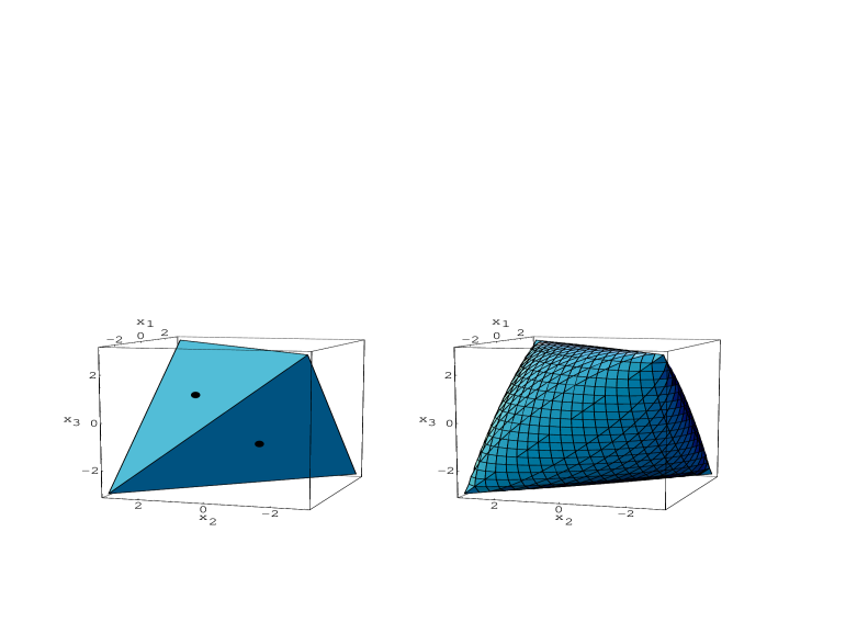
Figure 18: The fundamental domain (left) for constant gauge fields on $S^{3}$, with respect to the framing $\bar{e}_{\mu}^{j}$, in the diagonal representation $A_{j}=x_{j}\sigma_{j}$ (no sum over $j$). The dots on the faces indicate the sphalerons. On the right we show the Gribov horizon, which encloses the fundamental domain, coinciding with it at the singular boundary points along the edges of the tetrahedron.

In Fig. 18 we present the results for $\Lambda$ and $\Omega$. In this particular case, where $d=0$, $\Lambda$ coincides with $\tilde{\Lambda}$, a consequence of the convexity and the fact that both the sphalerons (indicated by the dots) and the edges of the tetrahedron lie on $\partial\Lambda$, the latter also lying on $\partial\Omega$. It is essential that the sphalerons do not lie on the Gribov horizon and that the potential energy near $\partial\Omega$ is relatively high. This is why we can take the boundary identifications near the sphalerons into account without having to worry about singular boundary points, as long as the energies of the low-lying states will be not much higher than the energy of the sphaleron. It allows one to study the glueball spectrum as a function of the CP violating angle $\theta$, but more importantly it incorporates for $\theta=0$ the noticeable influence of the barrier crossings, i.e. of the instantons.

An effective hamiltonian for the $c$ and $d$ modes is derived from the one-loop effective action.[132] To lowest order it is given by

$$H=-\frac{g^{2}(R)}{4\pi^{2}R}\left(\left(\frac{\partial}{\partial c_{i}^{a}}\right)^{2}+\left(\frac{\partial}{\partial d_{i}^{a}}\right)^{2}\right)+\frac{1}{g^{2}(R)R}\mbox{$\cal V$}(c,d)+\frac{1}{R}\mbox{$\cal V$}^{(1)}_{\rm eff}(c,d),$$ (86)

where $g(R)$ is the running coupling constant (related to the MS running coupling by a finite renormalization, such that the kinetic term in Eq. (86) has no corrections). The one loop correction to the effective potential is given by

$$\mbox{$\cal V$}^{(1)}_{\rm eff}(c,d) = \mbox{$\cal V$}^{(1)}_{\rm eff}(c)+\mbox{$\cal V$}^{(1)}_{\rm eff}(d)+\kappa_{7}(c^{a}_{i})^{2}(d^{b}_{j})^{2}+\kappa_{8}(c^{a}_{i}d^{a}_{j})^{2},$$

$$\mbox{$\cal V$}^{(1)}_{\rm eff}(c) = \kappa_{1}(c^{a}_{i})^{2}+\kappa_{2}\det c+\kappa_{3}(c^{a}_{i}c^{a}_{i})^{2}+\kappa_{4}(c^{a}_{i}c^{a}_{j})^{2}$$

$$+\kappa_{5}(c^{a}_{i})^{2}\det c+\kappa_{6}(c^{a}_{i}c^{a}_{i})^{3}.$$

with the following numerical values for the coefficients

$$\kappa_{1}=-0.24534599851796, \kappa_{5}=-0.84996541224534,$$

$$\kappa_{2}=+3.66869179814223, \kappa_{6}=-0.06550330854836,$$

$$\kappa_{3}=+0.50070320309661, \kappa_{7}=-0.36171221599671,$$

$$\kappa_{4}=-0.83935963341300, \kappa_{8}=-2.29535686135471.$$ (88)

Along the tunneling path (e.g. $c_{i}^{a}=-u\delta_{i}^{a}$ and $d=0$) the effective potential can be calculated with simpler methods, providing an important check.

Unlike for the torus, where in lowest order all excitations in the zero-momentum modes are degenerate and Bloch perturbation theory [24] provides a rigorous definition of the effective hamiltonian, one has to rely here on an adiabatic approximation not controlled by the coupling constant. The low lying excitations in the $c$ and $d$ modes are well below the excitations of the modes that were integrated out, justifying the adiabatic approximation.[126, 132] It provides enough room to achieve a satisfactory understanding of the non-perturbative dynamics due to spreading of the wave functional to the boundary of the fundamental domain. The boundary conditions are chosen such that the gauge and (left and right) rotational invariances are preserved and that they coincide with the appropriate boundary conditions near the sphalerons. Projection on the irreducible representations of these symmetries is essential to reduce the size of the matrices to be diagonalized in a Rayleigh-Ritz analysis. All this could be implemented in a tractable way,[132] see Fig. 19.

Figure 19: The full one loop results for the masses of scalar, tensor and odd glueballs on $S^{3}$ as a function of $f=g^{2}(R)/2\pi^{2}$ for $\theta=0$. The dashed lines correspond to the perturbative result.

In perturbation theory the $0^{-}$ “oddball” is slightly lighter than the $0^{+}$ glueball state. In lowest order the $0^{+}$, $0^{-}$ and $2^{+}$ glueball states are all degenerate, lifted in the next order in perturbation theory, by an amount independent of the one loop corrections

$$(m_{0^{-}}-m_{0^{+}})R = -g^{2}(R)/4\pi^{2}+\mbox{$\cal O$}\left(g^{4}\right),$$

$$(m_{2^{+}}-m_{0^{+}})R = 5g^{2}(R)/6\pi^{2}+\mbox{$\cal O$}\left(g^{4}\right),$$ (89)

whereas $m_{0}^{+}R=4-(1.25-\kappa_{1})g^{2}(R)/2\pi^{2}+\mbox{$\cal O$}\left(g^{4}\right)$. This perturbative result was also found by Diekmann.[133] (His one loop corrections, however, do not survive the test of reproducing the effective potential along the tunneling path.) Clearly, the $0^{-}$ glueball being the lightest state is an artifact of the finite volume, and it is an important test to see if non-perturbative effects that set in when going to larger volumes are able to correct for this unwanted feature. Indeed, when including the effects of the boundary of the fundamental domain, the $0^{-}/0^{+}$ mass ratio rapidly increases from slightly below 1 to above. At the same time the slow rise of the $2^{+}/0^{+}$ mass ratio becomes more rapid. This behavior is observed both with and without the one loop corrections included. In the latter case the non-perturbative effects set in at $g(R)\sim 2$. Beyond $g(R)\sim 2.8$ it can be shown that the wave functionals start to feel parts of the boundary of the fundamental domain which the present calculation is not representing properly. This value of $g(R)$ corresponds to a circumference of roughly 1.3 fm, when setting the scale as for the torus, assuming the scalar glueball mass in both geometries at this intermediate volume to coincide. That instanton effects are largely responsible for the spin splittings is further confirmed by studies in the instanton liquid model,[134] which concludes that instantons lead to an attractive, neutral and repulsive force in respectively the scalar, tensor and pseudo scalar glueball channels.[135]

6 Large Volume Results

We divide $\cal A$ by the set of all gauge transformations $\cal G$, including those that are homotopically non-trivial, to get the physical configuration space. All the non-trivial topology is then retrieved by the identifications of points on the boundary of the fundamental domain. This becomes important when the wave functional spreads out in configuration space, which happens at large volumes, whereas at very small volumes the wave functional is localized around $A=0$ and one need not worry about these non-perturbative effects. That these effects can be dramatic, even at relatively small volumes (above a tenth of a fermi across), was demonstrated for the case of the torus. It has historically been very important that the torus with periodic boundary conditions provides a relatively wide window, from a tenth of a fermi to three quarters of a fermi, where these non-perturbative effects can reliably be taken in to account, and were carefully verified in lattice Monte Carlo studies. It shows the intricate dynamics due to the intrinsic non-linearities of the theory and the fact that the issue of gauge copies can not be ignored and is important for the infrared dynamics of the theory.[4]

The hierarchy of boundary effects is effectively described by the various saddle points, that typically lie at the boundary of the fundamental domain. An important lesson can be learned from comparing different geometries, between which the structure of the fundamental domain deviate considerably. As we stressed before, the shape of the fundamental domain is independent of $L$ if the gauge field is expressed in units of $1/L$. It is only the strength of the coupling constant that controls the spreading of the wave functional. Suppose that the coupling constant will grow without bound. This would make the potential irrelevant and makes the wave functional spread out over the whole of field space (which could be seen as a strong coupling expansion). If the kinetic term would have been trivial, the wave functionals would be “plane waves” on a space with complicated boundary conditions. In that case it seems unavoidable that the infinite volume limit would depend on the geometry (like $T^{3}$ or $S^{3}$) that is scaled-up to infinity. Due to the non-triviality of the kinetic term this conclusion cannot be readily made and our present understanding only allows comparison in volumes around one cubic fermi. However, one way to avoid this undesirable dependence on the geometry is that the vacuum is unstable against domain formation. As periodic subdivisions are space filling on a torus, this seems to be the preferred geometry to study domain formation. It is hard to formulate this in a precise way, let alone find an order parameter for this domain formation. But let us assume domain formation does occur.

Since the ratio of the square root of the string tension to the scalar glueball mass shows no structure around $L=0.75$ fermi, we assume that within a domain both reach their large volume value. The color electric string now arises from the fact that flux that enters a domain has to leave it at the opposite side. Flux conservation with these building blocks automatically leads to a string picture, with a string tension as computed within a single domain and a transverse size of the string equal to the average size of a domain. The tensor glueball in an intermediate volume is heavily split between the doublet ($E^{+}$) and triplet ($T^{+}_{2}$) representations of the cubic group, with resp. 0.9 and 1.7 times the scalar glueball mass. This implies that the tensor glueball is at least as large as the average size of a domain. Rotational invariance in a domain-like vacuum comes about by averaging over all orientations of the domains. This is expected to lead to a mass which is the multiplicity weighted average of the doublet and triplet, yielding a mass of 1.4 times the scalar glueball mass. In the four dimensional euclidean context, $O(4)$ invariance makes us assume that domain formation extends in all four directions. The deconfining temperature would again be set by the average domain size. As is implied by averaging over orientations, domains will not neatly stack. There will be dislocations which most naturally are gauge dislocations. A point-like gauge dislocation in four dimensions is an instanton, lines give rise to monopoles and surfaces to vortices. In the latter two cases most naturally of the $Z_{N}$ type. We estimate the density of these objects to be one per average domain size. We thus predict an instanton density of $3.2\,{\rm fm}^{-4}$, with an average size of $1/3$ fermi. For monopoles we predict a density of $2.4\,{\rm fm}^{-3}$. The SU(2) spectra in volumes around the domain size, for the sphere and the torus, are compatible with $m(2^{+})/m(0^{+})\sim 1.5$ and $m(0^{-})/m(0^{+})\sim 1.7$. In this picture, we would further predict $\sqrt{K}/m_{0^{+}}\sim 0.24$. All these results seem to give the right order of magnitude, close to the values one measures in a large volume,

$$m(2^{+})/m(0^{+})=1.46\pm 0.09,\quad\sqrt{K}/m_{0^{+}}=0.267\pm 0.009,$$

$$m(0^{-})/m(0^{+})=1.78\pm 0.24,$$ (90)

taken from a recent review by Teper.[136] It would be useful to have high-precision lattice Monte Carlo data around $L=1$ fermi. In this intermediate volume range, the nature of the states changes from being dominated by zero-momentum fields to genuine particle states. It is important to take this into account in choosing the proper variational basis for the operators in the analysis of the Monte Carlo data. It is not sufficiently appreciated that it is exactly this change of the nature of the states that can provide fundamental physical insight in the formation of the mass gap and the confining string.

The studies reported so far in small and intermediate volumes were from first principles. The volume plays the role of the control parameter to keep the strength of the interactions in check. The challenge is to find which are the effective degrees of freedom that drive the formation of the mass gap. The lesson we learned is that large field fluctuations are essential. They enter as sphaleron configurations in the hamiltonian formulation, and are thus associated with instantons. Nevertheless, it seems inescapable that instantons, monopoles and vortices all have to be part of the equation,[137] in one way or another.

6.1 Volume Dependence of Stable Particle Masses

Once a mass gap is being formed, this gives of course the relevant degrees of freedom to describe the large distance behavior. For the torus, isolating the volume dependence to come from the propagator winding around the boundary of the box, has led Lüscher to derive the exponential approach of stable particle masses.[12] The method makes cunning use of the fact that the finite volume propagator is given by $\Delta_{L}(x)=\sum_{n\in{\rm Z\!\!Z}^{4}}\Delta(x+nL)$, where $\Delta(x)$ is the propagator in the infinite volume. With a mass gap the sum over periods will converge, since $\Delta(x)\approx e^{-m|x|}$. Physically $\Delta(x+nL)$ can be identified with propagation from $0$ to $x$, going in addition $n$ times around the box. Going around only once gives the leading finite volume correction of the order $e^{-ML}$. The value of $M$ depends on the mass gap, and which type of virtual corrections contribute to the self-energy of the particle under consideration. Obviously, without interactions their would be no volume dependence.

Applying these ideas to QCD, one assumes that the long distance behavior is described by an effective theory. In the presence of light quarks this is of course the chiral effective lagrangian. For the calculation of the volume dependence of the glueball, it is assumed to be an effective scalar theory. Confinement implies that propagation of a quark around the boundary, unlike in a small volume, is not an option for large $L$ due to the confining string it has to stretch. Similarly, gluons are confined and thus cannot propagate around the volume. It is only the physical colorless states that can propagate around the box at large $L$. Therefore, the fractional periods that appear in the perturbative expansion with twisted boundary conditions, see Sec. 3.4, have no effect on the finite size corrections in a large volume. Indeed twisted boundary conditions are devised such that all gauge invariant quantities are strictly periodic.[9]

Vertex functions are not affected by the finite volume, and the expression of a Feynman diagram in a finite volume is exactly of the same form as in an infinite volume, except that integrating over the vertex positions is restricted to the finite volume. The exponential suppression is caused by the finite volume modification in the propagator, specific for periodic boundary conditions. For the sphere, due to the curvature of the manifold, there will be algebraic corrections, and the volume corrections are much harder to establish. To keep track of the volume dependence universal properties of one-particle irreducible vertex functions are studied. A general Feynman diagram $\cal D$ will correspond to the amplitude

$$\mbox{$\cal J$}_{L}(\mbox{$\cal D$})=\!\!\!\!\!\prod_{v\in\mbox{$\cal V$}\backslash v_{0}}\prod_{\mu=0}^{d}\int_{0}^{L_{\mu}}\!\!{\rm d}x_{\mu}(v)\exp(i\sum_{e}p(e)\cdot x(e)){\bf V}\prod_{\ell\in\mbox{$\cal L$}}\Delta_{L}(x(f(\ell))-x(i(\ell))),$$ (91)

where $p(e)$ are external momenta. The set of vertices $v$ ($v_{0}$ those that are connected to an external line) and propagators $\ell$ are denoted by $\cal V$ and $\cal L$. The product of all vertex factors (coupling constants) is given by ${\bf V}$.

To single out those contributions that correspond to propagating $n$ times around the box, one has to take into account the invariance

$$x(v)\rightarrow x(v)+m(v)L,\quad n(\ell)\rightarrow n(\ell)+m(f(\ell))-m(i(\ell)),$$ (92)

where $m_{\mu}(v)\in{\rm Z\!\!Z}$ and $n(\ell)$ occurs in the expansion of $\Delta_{L}(x)$. With graph theory Lüscher [12] showed that the sum over $n(\ell)$ splits in a sum over the orbits $[n]$ and a sum over the integers $m(v)$. Obviously one has $\sum_{m}\int_{0}^{L}dx=\int_{-\infty}^{\infty}dx$ and only the sum over the orbits remains, $\mbox{$\cal J$}_{L}(\mbox{$\cal D$})=\sum_{[n]}\mbox{$\cal J$}_{L}(\mbox{$\cal D$},[n])$,

$$\mbox{$\cal J$}_{L}(\mbox{$\cal D$},[n])=\prod_{v\in\mbox{$\cal V$}\backslash v_{0}}\prod_{\mu=0}^{d}\int_{-\infty}^{\infty}{\rm d}x_{\mu}(v)\exp(i\sum_{e}p(e)\cdot x(e)){\bf V}$$

$$\times\prod_{\ell\in\mbox{$\cal L$}}\Delta(x(f(\ell))-x(i(\ell))+n(\ell)L).$$ (93)

The advantage of this decomposition is that for the orbit $[n]=[0]$, this is precisely the infinite volume expression, i.e. $\mbox{$\cal J$}_{L}(\mbox{$\cal D$},[0])=\mbox{$\cal J$}_{\infty}(\mbox{$\cal D$})$. When $[n]\neq[0]$ there is net winding around the boundary, the length of the extra winding given by $W([n])$, thereby leading to an exponential suppression,

$$\mbox{$\cal J$}_{L}(\mbox{$\cal D$},[n])\approx\exp\bigl{[}-mL\kappa(\{p(e)\})W([n])\bigr{]}.$$ (94)

The constant $\kappa(\{p(e)\})$ measures, in units of the mass gap $m$, the lowest momentum flowing through the propagators, constrained by the fixed external momenta. For a self-energy graph $\kappa(\{p(e)\})={\scriptstyle{{1\over 2}}}\sqrt{3}$, with the external momenta on-shell $p(e)=(im,{\bf 0})$, the only case needed here. Furthermore, $W([1])=1$ for a “simple” orbit $[1]$ (where $|n(\ell)|=1$, for one ling and 0 for all others) and $W([n])\geq\sqrt{2}$ for all other cases.[12]

To determine the finite volume corrections for the lightest stable one-particle state, one takes $L_{0}=\infty$ and $L_{j}=L$ (this simply implies we always have $n_{0}=0$). The mass is measured using $\langle\phi(t)\phi(0)\langle_{L}=\exp(-M(L)t)$, where $\phi(t)$ is an interpolating field for this state. This definition of the mass, also used in lattice calculations, coincides with the pole in the finite volume two-point function, $G_{L}^{-1}(iM(L),0)=0$. The two-point function $G_{L}(p)$ is defined by $G_{L}^{-1}(p)=p^{2}+m^{2}-\Sigma_{L}(p)$, where the normalization of the self-energy $\Sigma$ is such that $\Sigma_{\infty}(im,{\bf 0})={\partial^{2}\over\partial p^{2}}\Sigma_{\infty}(im,{\bf 0})=0$, which implies that in leading order $\delta M(L)=-{1\over 2m}(\Sigma_{L}-\Sigma_{\infty})(im,{\bf 0})=-{1\over 4m}\Gamma^{(2)}((im,{\bf 0}),[1])$. This can be expressed in terms of the full four-point Greens function by

$$\Gamma^{(2)}(p,[1])=\int{{\rm d}^{4}q\over(2\pi)^{3}}\left[6e^{iq_{1}L}G(q)\right]G^{(4)}(p,q,-p,-q),$$ (95)

where $\left[6e^{iq_{1}L}G(q)\right]$ comes from summing $\sum_{[n]=[1]}\mbox{$\cal J$}_{L}(\mbox{$\cal D$}_{2},[1])$ over the Feynman diagrams $\mbox{$\cal D$}_{2}$ that contribute to the full two-point function, and making use of the cubic invariance, to equate the contributions with $n_{j}=\pm 1$ to $n_{1}=1$.

The full four-point function can be related with the help of Schwinger-Dyson equations to the one-particle irreducible three- and four-point vertex functions. By shifts of integration contours, taking the analyticity domains of the vertex functions properly into account, one finds that the dominating contribution comes from the on-shell three-point vertex functions, denoted by $\lambda$, a physical three particle coupling constant. With $p=(im,{\bf 0})$, and both $q$ and $p+q$ “on-shell”, $q_{1}=i\sqrt{q_{\perp}^{2}+3m^{2}/4}$ and the integral over $q$, assuming the three point coupling does not vanish, can be shown to give [12]

$$\delta M(L)=-{3\lambda^{2}\over 16\pi m^{2}L}\exp(-{\scriptstyle{{1\over 2}}}\sqrt{3}mL)+\mbox{$\cal O$}\left(e^{-mL}\right).$$ (96)

The subleading term, of order $e^{-mL}$, is due to the contribution coming from the four-point function $\Gamma^{(4)}$.

The derivation has been given for the volume dependence of the mass gap, e.g. for the scalar glueball mass in pure gauge theory. The results also apply for the cases of a stable boundstate particle, with mass $m_{B}=2m-E_{B}$, and for a nucleon that couples to a pion. One only needs to adjust the “on-shell” condition, $q_{1}=i\sqrt{q_{\perp}^{2}+\mu_{B}^{2}}$, for the different kinematical situation. For the bound state one finds $\mu_{B}^{2}\equiv m^{2}-m_{B}^{2}/4$, which leads to $\delta M_{B}(L)=-3\lambda^{2}\exp(-\mu_{B}^{\vphantom{\dagger}}L)/(16\pi m_{B}^{2}L)$, whereas for the nucleon $\mu_{N}^{2}\equiv m_{\pi}^{2}-m_{\pi}^{4}/4m_{N}^{2}$, giving $\delta M_{N}(L)=-9m_{\pi}^{2}g_{N\pi}^{2}\exp(-\mu_{N}^{\vphantom{\dagger}}L)/(16\pi m_{N}^{2}L)$, where $\lambda$ has been expressed in the appropriate dimensionless pion-nucleon coupling constant $g_{N\pi}^{\vphantom{\dagger}}$. For the finite volume correction to the pion mass in QCD, the pion three-point vertex vanishes and one gets a slightly more complicated results of order $\exp(-m_{\pi}L)$, involving an integral over the forward scattering amplitude.[12]

6.2 Volume Dependence from Scattering Phase Shifts

Also it was shown by Lüscher how to extract scattering phase shifts from volume dependence.[138, 139] A less rigorous method, based on the notion of pseudo potentials, allows for a transparent way of understanding this all order result.[140] Consider the reduced hamiltonian $H=-m^{-1}\partial_{{\bf x}}^{2}+V({\bf x})$ for two interacting particles in the center of mass in ordinary quantum mechanics with a (Bose) symmetric reduced wave functions, $\psi({\bf x})=\psi(-{\bf x})$. When the potential has a finite range $\lambda$ ($V({\bf x})=0$ for $|{\bf x}|>\lambda$), the wave function is a plane-wave outside of the interaction region. Scattering theory tells us there is a unique relation between the incoming wave $e^{-ip|x|}$ and the outgoing wave $e^{ik|x|}$ in terms of the scattering phase shift $\delta(k)$

$$\psi(x)=e^{-ik|x|}+e^{2i\delta(k)}e^{ik|x|},\quad|x|>\lambda.$$ (97)

These states form a complete basis of scattering states. In a finite volume the periodic boundary condition, $\psi(x+L/2)=\psi(x-L/2)$, implies the following implicit equation for the momenta

$$e^{2i\delta(k)}e^{ikL}=1,$$ (98)

which holds as long as $L>2\lambda$, showing how the volume dependence of two-particle states are related to the phase shift. For a vanishing potential the phase shift vanishes, $\delta(k)=0$, and one recovers the standard discretization of the momenta, $k=2\pi n/L$.

In more than one dimension a complete set of scattering wave functions is given by

$$\psi^{({\bf k})}_{\ell m}({\bf x})=[j_{\ell}(|{\bf k}|r)-\tan(\delta_{\ell}({\bf k}))n_{\ell}(|{\bf k}|r)]Y_{\ell m}(\hat{\bf k}),$$ (99)

where $\hat{\bf k}={\bf k}/|{\bf k}|$, $r=|{\bf x}|$ and $j_{\ell}$, $n_{\ell}$ are the spherical Bessel-functions. The energy is given by $E={\bf k}^{2}/m$. It appears that the spherical nature of the scattered waves makes it impossible to impose periodic boundary conditions. One can, however, introduce the notion of a pseudo potential as was introduced for the hard-sphere bose gas by Huang and Yang.[141] The essential idea is equally simple as powerful. Replace $V({\bf x})$ by the simple pseudo potential $V_{\delta}({\bf x})$ such that for $|{\bf x}|>\lambda$, eq. ((99)) is still an exact solution of the relevant Schrödinger equation. Subsequently one solves the Schrödinger equation with $V_{\delta}$ as its (energy dependent) potential, using periodic boundary conditions. We illustrate this by making the simplified assumption that all phase shifts vanish, except for $\delta_{0}$. In that case one easily verifies that the pseudopotential is given by

$$V_{\delta}({\bf x})=-{4\pi\over mk}\tan(\delta_{0}({\bf k}))\hat{\delta}_{3}({\bf x}).$$ (100)

Since we have to allow for wave functions that are singular at the origin, we can extend our class of functions to those that, when averaged over the angles, have a Laurent expansion $\sum_{n=-N}^{\infty}c_{n}r^{n}$. We define $\hat{\delta}_{3}({\bf x})\psi({\bf x})=c_{0}\delta_{3}({\bf x})$. Alternatively, $\hat{\delta}_{3}({\bf x})\psi({\bf x})={\partial\over\partial r}(r\psi({\bf x}))\delta_{3}({\bf x})$. We expand the wave function in plane waves, suitable for implementing periodic boundary conditions, $\psi({\bf x})=L^{-3}\sum b_{{\bf n}}\exp(2\pi i{\bf x}\cdot{\bf n}/L)$. Substituting this in the relevant Schrödinger equation

$$(-{1\over m}{\partial^{2}\over\partial{\bf x}^{2}}+V_{\delta}({\bf x}))\psi({\bf x})={{\bf k}^{2}\over m}\psi({\bf x}),$$ (101)

is easily seen to give

$$b_{{\bf n}}=-{4\pi\tan(\delta_{0}({\bf k}))\over|{\bf k}|({\bf k}^{2}-(2\pi{\bf n}/L)^{2})}c_{0}.$$ (102)

With $c_{0}=\sum b_{{\bf n}}$ we thus find a relation between the momentum in the center of mass and the scattering phase shift at this momentum

$${\tan(\delta_{0}({\bf k}))\mbox{$\cal Z$}_{00}(1;{\bf q})\over 2\pi^{2}|{\bf q}|}=1,\quad{\bf q}={{\bf k}L\over 2\pi}.$$ (103)

The zeta-function $\mbox{$\cal Z$}_{00}(s;{\bf q})\equiv\sum_{{\bf n}\in{\rm Z\!\!Z}^{3}}({\bf n}^{2}-{\bf q}^{2})^{-s}$ is defined through analytic continuation in $s$.

To obtain this result $c_{0}$ should be non-vanishing. There can be “singular” solutions [139] for which $c_{0}=0$ at momenta ${\bf k}=2\pi{\bf n}/L$, if there exists ${\bf n}^{\prime}\in{\rm Z\!\!Z}^{3}$, such that $|{\bf n}|=|{\bf n}^{\prime}|$. In that case $\psi({\bf x})=\exp(2\pi i{\bf n}\cdot{\bf x}/L)-\exp(2\pi i{\bf n}^{\prime}\cdot{\bf x}/L)$ is regular and vanishes in the origin. If $\psi$ is in the scalar representation ($A_{1}$) of the cubic group, this singular behavior only occurs when ${\bf n}^{\prime}$ is not related to ${\bf n}$ by a cubic transformation, which will make the momentum where this occurs quite large. Furthermore, restricting to the $A_{1}$ sector, eq. ((103)) will also be valid if the phase shifts only vanish for angular momenta $\ell\geq 3$. This is because a spin 2 wave function decomposes in the $E$ and $T_{2}$ representations of the cubic group and hence does not couple to the scalar sector (note that due to the Bose symmetry all odd angular momentum phase shifts will vanish).

In field theory it can be shown that the reduced hamiltonian is replaced by an effective Schrödinger equation, that can be derived from the Bethe-Salpeter equation for the four-point function.[138] Its energy-dependent “potential” is proportional to the so-called Bethe-Salpeter kernel, with the range $\lambda$ determined by the polarization cloud (which is why we restrict the analysis to field theories with a mass gap). The fully relativistic two-particle energy $W$ is given by $W=2\sqrt{{\bf k}^{2}+m^{2}}=2\sqrt{m(m+E)}$, where ${\bf k}$ is the center of mass momentum of the scattering pair. Lüscher’s [139] all order analysis is based on studying the solutions of the Helmholtz equation $(\partial^{2}/\partial{\bf x}^{2}+{\bf k}^{2})\psi({\bf x})=0$ in a finite volume, allowing for power-like singularities at the origin. He demonstrates that truncating to a finite number of phase shifts $\delta_{\ell}$, ($\ell<\ell_{max}$) in general converges rapidly with $\ell_{max}$. For the simplified case that only $\delta_{0}$ is non-vanishing, the result is as in Eq. (103).

One of the applications is computing the energy of the two-particle states as a function of $L$. Using

$$\mbox{$\cal Z$}_{00}(1;{\bf q}) = -{1\over{\bf q}^{2}}+Z_{00}(1;{\bf 0})+{\bf q}^{2}Z_{00}(2;{\bf 0})+\mbox{$\cal O$}\left(q^{4}\right),$$

$$\tan(\delta_{0}({\bf k})) = a_{0}|{\bf k}|+\mbox{$\cal O$}\left(k^{3}\right),$$ (104)

introducing $Z_{00}(s;{\bf q})=\mbox{$\cal Z$}_{00}(s;{\bf q})-(-{\bf q}^{2})^{-s}$ and $a_{0}$, the so-called the scattering length. One can now straightforwardly iterate eq. ((103)) and find

$${\bf k}^{2} = -{4\pi a_{0}\over L^{3}}(1+{c_{1}a_{0}\over L}+{c_{2}a_{0}^{2}\over L^{2}})+\mbox{$\cal O$}\left(L^{-6}\right),$$ (105)

$$c_{1} = {Z_{00}(1;{\bf 0})\over\pi},\quad c_{2}={Z_{00}^{2}(1;{\bf 0})-Z_{00}(2;{\bf 0})\over\pi^{2}}.$$

The numerical values [138, 141] are $c_{1}=-2.837297$ and $c_{2}=6.375183$. When the two-particle energies come close to the mass of a resonance, like the $\rho$ or $K$ meson coupling to two-particle pion states, the phase shifts get large and it becomes imperative to use the all order results.[139]

Many of the aspects of the large volume expansions for the one-particle and two-particle masses have been verified successfully for the two dimensional non-linear sigma [142] and Ising model [143], and for the four dimensional Ising [144] and O(4) $\phi^{4}$ model in the symmetric phase.[145] Recently the method has been revisited by Lellouch and Lüscher [146] for studying on the lattice non-perturbatively the decay $K\rightarrow\pi\pi$, important for understanding direct CP violation. By studying the decay in a finite volume, the transition amplitude of the kaon to the discrete set of finite volume two-pion final states can be related to the infinite volume decay rate. With the advance in computer power this calculation will be feasible in the future.

6.3 Goldstone Modes and Chiral Perturbation Theory

The finite size corrections to the string tension $K(L)$ also rely on an effective description, namely that of the bosonic relativistic string. The finite size behavior is described in terms of the force by

$$F(L)=\frac{dE(L)}{dL}=\frac{dLK(L)}{dL}=K+\frac{\pi}{3}L^{-2}+\mbox{$\cal O$}\left(L^{-3}\right),$$ (106)

with $K$ the infinite volume string tension. The so-called Lüscher term [147] with the $1/L^{2}$ correction is universal. A simple way to understand this correction is in terms of the Casimir energy in one space dimension (the string) on a periodic interval of length $L$ (the length of the string) for two massless scalar fields (the two independent transverse fluctuations of the string), $2\cdot{\scriptstyle{{1\over 2}}}\sum_{k}2\pi|k|/L=4\pi\zeta(-1)/L$ (in dimensional regularization, with $\zeta$ the Riemann zeta function). Lüscher’s original derivation was for a string with fixed end-points, for which the Casimir energy is a quarter of the one with periodic boundary conditions. The transverse fluctuations are examples of Goldstone bosons, that here arise due to the spontaneous breakdown of the transverse translational invariance in the background of a string.[147]

Goldstone bosons do of course also play a very important role in the low-energy description of QCD in the form of pions. They occur with massless quarks due to the spontaneous breakdown of chiral symmetry. With an explicit mass term for the quarks, the pions acquire a mass and the results of Secs. 6.1 and 6.2 apply as long as $m_{\pi}L\gg 1$. For massless pions this can of course not be realized, and instead chiral perturbation theory becomes an effective tool. It also applies for $m_{\pi}\neq 0$ provided $L$ is in the so-called mesoscopic range, which is $m_{\pi}^{-1}\gg L\gg\Lambda_{QCD}^{-1}$. The principle behind chiral perturbation theory is that the symmetries of the low-energy theory strongly constrain the effective lagrangian. The resulting sigma model has its symmetry determined by the number of light quark flavors and the gauge group. For SU(3) with two light flavors, the up and the down quark, this is the O(4) sigma model spontaneously broken down to O(3) by the chiral condensate. Finite size effects occur in powers of $1/L$, but are determined by infinite volume quantities, computed essentially through replacing the continuous by discrete momenta.[148]

From the practical point of view this gives access to these infinite volume quantities through finite size effects. An important example is the chiral condensate, which can be related through the Leutwyler-Smilga sum rules [149] to eigenvalue distributions of the Dirac operator (averaging over the gauge fields). It is the average spacing of these eigenvalues near zero that through the Banks-Casher formula [150] gives access to the chiral condensate $\langle\Delta\lambda\rangle=\pi(L^{3}T|\langle\overline{\psi}\psi\rangle|)^{-1}$. The roughness of the gauge field causes $\langle\Delta\lambda\rangle$ to be inversely proportional to the volume ($L^{3}T$) of space-time. At weak coupling, like in a small volume, the typical eigenvalue spacing would be $1/L$, but in addition we saw in Sec. 3.2 there are no near zero eigenvalues and chiral symmetry is manifest.

Remarkably, in the mesoscopic domain the low-lying eigenvalue distribution $\langle\rho(\lambda)\rangle$ is related to a universal function called the microscopic spectral density,[151] $\rho_{S}(u)=\lim_{V\rightarrow\infty}(V\Sigma)^{-1}\langle\rho\left((V\Sigma)^{-1}u\right)\rangle$. It can be calculated in Random Matrix Theory, leaving the chiral condensate $\Sigma=|\langle\overline{\psi}\psi\rangle|$ as a single free parameter. We refer to a review by Verbaarschot [152] for details.

6.4 Electric-Magnetic Duality

Much of the finite volume work in gauge theories has started with ’t Hooft’s paper on the torus with twisted boundary conditions.[9] We come back to it one more time to show how it leads to an electric-magnetic duality, which can be used to derive finite size results for the energy of magnetic flux in terms of the string tension, assuming one has a confining string.

Consider the gauge group SU($N$) and fix the magnetic flux ${\bf m}$ by twisted boundary conditions. In the $A_{0}=0$ gauge this can be specified as in Eq. (31). Given these boundary conditions, the remaining gauge freedom is specified by the twisted gauge transformations $h_{\bf k}$, defined in Eq. (35), where ${\bf k}$ classifies the element of the homotopy group $H_{2}(T^{3},Z_{N})\sim Z_{N}^{3}$. Two twisted gauge transformations with the same value of ${\bf k}\in Z_{N}^{3}$ differ by a gauge transformation with integer winding number. A particular representative of $h_{{\bf k}}$ can be chosen such that [50] $\nu(h_{{\bf k}})=-{\bf k}\cdot{\bf m}/N$, as we argued below Eq. (50). The generalization of Eq. (20) to ${\bf m}\neq{\bf 0}$ can now be written as

$$\Psi([h_{{\bf k}}h_{1}^{\nu}]\,A)=e^{i\theta\nu}\exp\left(\frac{2\pi i{\bf e}^{\vphantom{\dagger}}_{\theta}\cdot{\bf k}}{N}\right)\Psi(A),\quad{\bf e}^{\vphantom{\dagger}}_{\theta}\equiv{\bf e}-\frac{\theta}{2\pi}{\bf m}.$$ (107)

The non-trivial $\theta$ dependence implies that magnetic flux will carry in general a fractional electric flux. This result is intimately related to the observation of Witten [153] that the $\theta$ dependence can be implemented at the hamiltonian level, by replacing the canonical momentum belonging to the gauge field, i.e. the electric field $E_{i}({\bf x})$, by $E_{i}({\bf x})-\frac{\theta}{4\pi^{2}}B_{i}$, with $B_{i}({\bf x})\equiv{\scriptstyle{{1\over 2}}}\epsilon_{ijk}F_{jk}({\bf x})$ the magnetic field. This behavior, of magnetic charge obtaining a $\theta$ dependent electric charge, also plays a role in ’t Hooft’s abelian projection and oblique confinement.[154]

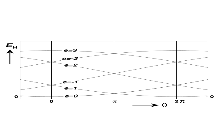
Figure 20: The SU(6) spectral flow [72] of $E_{\theta}^{\vphantom{\dagger}}$ in a small volume, Eq. (108), representing the energy of electric flux for ${\bf m}=(0,0,1)$ and $e_{1}=e_{2}=0$. The spectrum is periodic with a period $2\pi$, the flow only with a period of $12\pi$.

It seems that the $2\pi$ periodicity in $\theta$ needs to be replaced by $2\pi N$. Nevertheless, the spectrum itself is periodic with period $2\pi$. There is, however, a non-trivial spectral flow, which in the infinite volume may be non-analytic and give rise to oblique confinement.[154] The spectral flow can neatly be illustrated in a finite volume, where energies are required to be analytic in $\theta$. For this we consider ${\bf m}=(0,0,1)$ and recall from Sec. 3.4 that the energy splittings for ${\bf e}=(0,0,e_{3})$ are due to tunneling with fractionally charged instantons. One easily computes the resulting energies through standard instanton calculations,[155, 156] using the fact that the twisted instanton has only four zero-modes due to translations (cmp. Sec. 4),

$$E^{\vphantom{\dagger}}_{\theta}({\bf e}=e{\bf m}=e{\bf e}^{(3)})=\mbox{$\cal C$}\sin^{2}(\pi|{\bf e}^{\vphantom{\dagger}}_{\theta}|/N)\exp\bigl{[}-8\pi^{2}/Ng^{2}(L)\bigl{]}/Lg^{4}(L).$$ (108)

The behavior of $E^{\vphantom{\dagger}}_{\theta}$ is illustrated, for $N=6$, in Fig. 20 from which it is immediately clear that the spectrum is periodic with a period of $2\pi$, but that following the energy levels adiabatically, one only returns to the same situation after $N=6$ periods.

We now consider the euclidean partition function at finite temperature, specified by $1/\beta$, where $\beta$ is the period in the euclidean time direction. For simplicity we will also assume the period lattice $\Xi$ is orthogonal, $a^{(\mu)}=L_{\mu}e^{(\mu)}$ with $L_{0}\equiv\beta$. The free energy $F({\bf e},{\bf m},L_{\mu})$ is defined for the different superselection sectors as

$$\exp\left[-\beta F_{\theta}({\bf e},{\bf m},L_{\mu})\right]=\mbox{\,Tr\,}^{\vphantom{\dagger}}_{\theta,{\bf e}}\left[\exp(-\beta H^{\vphantom{\dagger}}_{\bf m})\right],$$ (109)

where the trace is here over the Hilbert space with definite $\theta$, electric and magnetic quantum numbers. To relate the finite temperature partition function to the euclidean path integral, $\theta$ and the electric flux have to be implemented as a sum over the homotopy classes ($\nu\in{\rm Z\!\!Z}$ and ${\bf k}\in Z_{N}^{3}$) of the gauge transformations. In the $A_{0}=0$ gauge, the gauge field at $t=0$ is related to that at $t=\beta$ by $A({\bf x},\beta)=[h_{{\bf k}}h_{1}^{\nu}]\,A({\bf x},0)$. For a given choice of $\nu$ and ${\bf k}$ we denote the euclidean path integral by $W_{\nu}({\bf k},{\bf m},L_{\mu})=W_{\nu}(n,\Xi)$, where $n$ denotes the antisymmetric integer twist tensor, with $n_{ij}=\epsilon_{ijl}m_{l}$ and $n_{0i}=k_{i}$ specifying the twisted boundary conditions, which can now be formulated in any gauge. The relation between the free energy and the euclidean path integral reads

$$\exp[-\beta F_{\theta}({\bf e},{\bf m},L_{\mu})]=N^{-3}\sum_{{\bf k}\in Z_{N}^{3}}\sum_{\nu\in{\rm Z\!\!Z}}e^{i\nu\theta}{\rm z}_{{}_{N}}^{-{\bf k}\cdot{\bf e}_{\theta}}W_{\nu}({\bf k},{\bf m},L_{\mu}),$$ (110)

where we introduced the $N$-th root of unity, ${\rm z}_{{}_{N}}\equiv e^{2\pi i/N}$.

The alternate notation, $W_{\nu}(n_{\mu\nu},\Xi)$, makes manifest that from the point of view of the euclidean path integral there is no essential distinction between the twisted boundary conditions in the space and the time directions. As observed by ’t Hooft, this path integral is invariant under a joint SO(4) rotation of the period lattice $\Xi$ and the twist tensor $n$. This nearly trivial fact, however, results in a duality between the electric and magnetic sectors. [9] A simultaneous rotation in the 1-2 and the 3-0 planes over 90 degrees, interchanges $(k_{1},k_{2})$ with $(m_{1},m_{2})$, leaves $k_{3}$ and $m_{3}$ unchanged and maps $L_{\mu}$ to $\tilde{L}_{\mu}=(L_{3},L_{2},L_{1},\beta)$. Substituting this in Eq. (110) leads to the exact duality [9]

$$\exp[-\beta F_{\theta}({\bf e},{\bf m},L_{\mu})]=N^{-2}\!\!\!\!\!\!\sum_{\tilde{\bf m},\tilde{\bf e}\in Z_{N}^{3}}\!\!\!\!\!\delta_{\tilde{m}_{3}m_{3}}\delta_{\tilde{e}_{3}e_{3}}\,{\rm z}_{{}_{N}}^{\tilde{\bf e}\cdot{\bf m}-\tilde{\bf m}\cdot{\bf e}}\exp[-L_{3}F_{\theta}(\tilde{\bf e},\tilde{\bf m},\tilde{L}_{\mu})].$$ (111)

It is because $\tilde{\bf e}_{\theta}\cdot{\bf m}-\tilde{\bf m}\cdot{\bf e}_{\theta}$, is independent of $\theta$, that $\theta$ does not explicitly appear in this equation.[73] Hence, we will in the following ignore the $\theta$ label.

Let us normalize $F({\bf 0},{\bf 0},L_{\mu})=0$, and call those flux states for which $L_{\mu}F({\bf e},{\bf m},L_{\mu})$ tends to zero light fluxes. That they cannot all be light is easily seen by summing Eq. (111) over $m_{1}$, $m_{2}$, $e_{1}$ and $e_{2}$,

$$N^{-2}\sum_{e_{1},e_{2},m_{1},m_{2}}\exp[-\beta F({\bf e},{\bf m},L_{\mu})]=\exp[-L_{3}F(e_{3}{\bf e}^{(3)},m_{3}{\bf e}^{(3)},\tilde{L}_{\mu})].$$ (112)

If $(e_{3}{\bf e}^{(3)},m_{3}{\bf e}^{(3)})$ produces a light flux state, there must be $N^{2}-1$ additional light flux states (with the same $e_{3}$ and $m_{3}$). On the other hand, since the euclidean path integral is positive, irrespective the twist, once the flux $({\bf e},{\bf m})$ is light, so must be the flux $({\bf 0},{\bf m})$ (see Eq. (110)). For SU(2) and SU(3) it can thus be concluded [9] that, in the confined phase, the magnetic fluxes have a vanishing free energy in the infinite volume limit.

It will be assumed that for $\beta\gg L_{i}$ the free energy factorizes in a magnetic and electric component, $F({\bf e},{\bf m},L_{\mu})=F_{m}({\bf m},L_{\mu})+F_{e}({\bf e},L_{\mu})$. This can be justified by the fact that the electric flux is squeezed into a string with a finite width (to give rise to a linear potential), which at high $\beta$ takes negligible space, whereas magnetic flux spreads out over the whole volume (for the free energy to vanish). We now show how to compute the volume dependence of the magnetic energy, $E_{m}({\bf m},L_{i})\equiv\lim_{\beta\rightarrow\infty}(F_{m}({\bf m},L_{\mu})-F_{m}({\bf 0},L_{\mu}))$, for the case where $m_{3}=0$. Let us choose $e_{3}=0$ and (for simplicity) $L_{1}=L_{2}=L$, with $\beta,L_{3}\gg L$. From Eq. (111) it follows that

$$\mbox{$\cal C$}\exp[-\beta F_{m}({\bf m}_{\perp},L_{\mu})]=N^{-2}\sum_{\tilde{\bf e}_{\perp}\in Z_{N}^{2}}{\rm z}_{{}_{N}}^{\tilde{\bf e}_{\perp}\cdot{\bf m}_{\perp}}\exp[-L_{3}F_{e}(\tilde{\bf e}_{\perp},\tilde{L}_{\mu})].$$ (113)

The normalization constant $\cal C$ (obtained by putting ${\bf m}={\bf 0}$) can be absorbed in $F_{m}$. One can compute the electric free energies from the statistical distribution of flux strings of energy $KL$, running in either the 1- or 2-direction, to build up the fluxes $e_{i}$ from $n_{i}+e_{i}$ strings running in the $i$-direction and $n_{i}$ in the opposite direction. For SU(2), fluxes running in opposite directions are equivalent, and one instead sums over $n_{i}$ even for $e_{i}=0$ and $n_{i}$ odd for $e_{i}=1$. Entropy allows us to ignore higher units of electric flux (including the ones running diagonally). Strings running in the long 3-directions can be neglected as well. The Boltzmann weight of one string equals $LL_{3}\exp(-\beta KL)/\mbox{$\cal A$}$, where $\cal A$ is a constant related to the “proper area” of the string. It is now straightforward to compute the electric free energy, substitute the result in Eq. (113) and obtain [9] the magnetic energy by extracting the limiting behavior in $\beta\rightarrow\infty$,

$$E_{m}=2(2-\delta_{N,2})\bigl{[}\sin^{2}(\pi m_{1}/N)+\sin^{2}(\pi m_{2}/N)\bigr{]}\mbox{$\cal A$}^{-1}L\exp(-LL_{3}K).$$ (114)

Thus the magnetic energy falls off in leading order with the same area law as the Wilson loop expectation value.

7 Conclusions

I have tried to convince the reader of the usefulness of a finite volume as a control in studying four dimensional non-abelian gauge theories, with for the torus the practical benefit of providing a guide for lattice Monte Carlo results. There are many issues I have not addressed here. Needless to say the choices have been determined by the things I have worked on in the past, or that were close to me. I hope to have at least succeeded in developing this theme here in a logical and pedagogical fashion. It is my belief that probing the non-perturbative dynamics through spectral properties is the only reliable way to gain insight. This is not to say it is only through finite volume studies we may make progress. There is of course the large $N$ expansion,[158, 159] and the hope for a string representation of QCD.[160] It should also be said we have followed the standard paradigm, that confinement is first to be understood in the pure gauge sector, instead of taking the attitude that the light quarks provided by nature is what mostly matters.[157]

On the basis of this review we list a number of open problems that are worthwhile addressing.

1. Solve the problem with the adiabatic approximation in the calculation of the Witten index in small volume supersymmetric gauge theories.

2. Find analytic solutions for the basic instantons on the torus, with and without twist.

3. Isolate the associated sphaleron configurations and non-perturbatively important degrees of freedom.

4. Map out with high-precision the low-lying spectrum around 1 fermi.

5. Establish in a reliable way the physical nature of the finite volume cross-over near 1 fermi, and find the intermediate-distance effective degrees of freedom, that are responsible for the mass gap and string formation.

The first two items are interesting technical problems in their own, which one may hope are close to being solved. They have a wider range of applications than in the context of QCD alone. The fourth item does not have to wait for analytic predictions, and can be addressed by Monte Carlo methods with present day resources. The last item is of course what it is all about. It is unlikely this can be solved by a single mathematical equation, or with mathematical rigor.[161] Fortunately, we do have experiment to guide us here. Despite the many phenomenological models, victory can not be claimed yet. The scenario of Mandelstam and ’t Hooft, for describing QCD in terms of a dual superconductor,[162, 163] remains an appealing one and gets some support from supersymmetric gauge theories exhibiting Seiberg-Witten duality,[164] even though their matter content is uncomfortably far from that of QCD.

The challenge of really understanding QCD non-perturbatively remains wide open, even though many in the particle physics community escape to other dimensions. Some of them hope that from this higher vantage point we can look down upon this problem that was left over from the twentieth century, and solve it with twenty-first century techniques. Anything is allowed, as long as we come up with a practical and reliable solution.

References

References

- [1] C.N. Yang and R.L. Mills, Phys. Rev. 96, 191 (1954).
- [2] N.M. Christ and T.D. Lee, Phys. Rev. D 22, 939 (1980).
- [3] O. Babelon and C. Viallet, Comm. Math. Phys. 81, 515 (1981).
- [4] V.N. Gribov, Nucl. Phys. B 139, 1 (1978).
- [5] M.A. Semenov-Tyan-Shanskii and V.A. Franke, Zapiski Nauchnykh Sem. Leningradskogo Otdeleniya Mat. Inst. im. V.A. Steklov AN SSSR 120, 159 (1982), Translation (Plenum, New York, 1986) p 999.
- [6] J.D. Bjorken, “Elements of Quantum Chromodynamics”, in Slac Summer Institute on Particle Physics, ed. A. Mosher (SLAC, Stanford, 1980).
- [7] M. Lüscher, Nucl. Phys. B 219, 233 (1983).
-
[8]
M. Lüscher, R. Sommer, U. Wolff and P. Weisz,
Nucl. Phys. B 389, 247 (1993) (hep-lat/9207010);
Nucl. Phys. B 413, 481 (1994) (hep-lat/9309005). - [9] G. ’t Hooft, Nucl. Phys. B 153, 141 (1979).
- [10] E. Witten, Nucl. Phys. B 202, 253 (1982).
- [11] W. Nahm, Phys. Lett. B 90, 413 (1980); in Monopoles in Quantum Field Theory, eds. N. Craigie et al (World Scientific, Singapore, 1982); in Lect. Notes in Phys. vol 201, eds. G. Denardo et al (Springer, Berlin, 1985).
- [12] M. Lüscher in Progress in Gauge Field Theory, eds. G. ’t Hooft et al (Plenum, New York, 1984) p 451; Comm. Math. Phys. 104, 177 (1986).
- [13] H. Leutwyler, Chiral Dynamics, this volume (hep-ph/0008124).
- [14] G. Dell’Antonio and D. Zwanziger, Comm. Math. Phys. 138, 291 (1991); in Probabilistic Methods in Quantum Field Theory and Quantum Gravity, eds. P.H. Damgaard et al (Plenum, New York, 1990) p 107.
- [15] G. Dell’Antonio and D. Zwanziger, Nucl. Phys. B 326, 333 (1989).
- [16] D. Zwanziger, Nucl. Phys. B 378, 525 (1992).
- [17] P. van Baal, Nucl. Phys. B 369, 259 (1992).
- [18] J. Koller and P. van Baal, Nucl. Phys. B 302, 1 (1988).
- [19] P. van Baal, Nucl. Phys. B 307, 274 (1988) [erratum B312, 752 (1989)].
- [20] P. van Baal, Nucl. Phys. B 264, 548 (1986).
- [21] A. Belavin, A. Polyakov, A. Schwarz and Y. Tyupkin, Phys. Lett. B 59, 85 (1975).
- [22] G. ’t Hooft, Phys. Rev. D 14, 3432 (1976) [erratum D18, 2199 (1978)].
- [23] J. Koller and P. van Baal, Phys. Rev. Lett. 58, 2511 (1987).
- [24] C. Bloch, Nucl. Phys. 6, 329 (1958).
- [25] P. van Baal, Nucl. Phys. B 351, 183 (1991).
- [26] A. Auerbach, S. Kivelson and D. Nicole, Phys. Rev. Lett. 53, 411 (1984); A. Auerbach and S. Kivelson, Nucl. Phys. B 257, 799 (1985).
- [27] P. van Baal and A. Auerbach, Nucl. Phys. B 275, 93 (1986).
- [28] P. van Baal in Lectures on Path Integration, eds. H.A. Cerdeira et al (World Scientific, Singapore, 1993) p 54.
- [29] J. Koller and P. van Baal, Nucl. Phys. B 273, 387 (1986).
- [30] P. van Baal and J. Koller, Ann. Phys. (N.Y.) 174, 299 (1987).
- [31] M. Lüscher and G. Münster, Nucl. Phys. B 232, 445 (1984).
-
[32]
C. Vohwinkel, Phys. Lett. B 213, 54 (1988);
Nucl. Phys. B(Proc. Suppl.) 9, 242 (1989). -
[33]
M. García Pérez and P. van Baal,
Nucl. Phys. B 429, 451 (1994)
(hep-lat/9403026). - [34] B.A. Berg and A.H. Billoire, Phys. Lett. B 166, 203 (1986) [erratum B185, 446 (1987)]; B.A. Berg, A.H. Billoire and C. Vohwinkel, Phys. Rev. Lett. 57, 400 (1986).
- [35] C. Michael, G.A. Tickle and M.J. Teper, Phys. Lett. B 207, 313 (1988).
- [36] J. Kripfganz and C. Michael, Nucl. Phys. B 314, 25 (1989).
- [37] B.A. Berg, Phys. Lett. B 206, 97 (1988).
- [38] C. Michael, Phys. Lett. B 232, 247 (1989).
-
[39]
P. Hasenfratz, A. Hasenfratz and F. Niedermayer,
Nucl. Phys. B 329, 739 (1990). - [40] B.A. Berg and A.H. Billoire, Phys. Rev. D 40, 550 (1989).
- [41] C. Michael, Nucl. Phys. B 329, 225 (1990).
-
[42]
M. García Pérez, J. Snippe and P. van Baal,
Phys. Lett. B 389, 112 (1996) (hep-lat/9608036). - [43] B.A. Berg and C. Vohwinkel, Ann. Phys. (N.Y.) 204, 351 (1990).
- [44] C. Vohwinkel, Calculation of the Mass Spectrum and Deconfining Temperature in Non-Abelian Gauge Theory, PhD thesis (Tallahassee, September 1989).
-
[45]
P. van Baal, Phys. Lett. B 224, 397 (1989);
Nucl. Phys. B(Proc. Suppl.) 17, 581 (1990). - [46] P. Weisz and V. Ziemann, Nucl. Phys. B 284, 157 (1987).
- [47] J. Koller and P. van Baal, Phys. Rev. Lett. 57, 2783 (1986).
- [48] C. Vohwinkel, Phys. Rev. Lett. 63, 2544 (1989).
- [49] P. van Baal in Probabilistic Methods in Quantum Field Theory and Quantum Gravity, eds. P.H. Damgaard et al (Plenum, New York, 1990) p 31.
- [50] P. van Baal, Comm. Math. Phys. 85, 529 (1982).
- [51] J. Hoek, Nucl. Phys. B 332, 530 (1990).
- [52] J. Kripfganz and C. Michael, Phys. Lett. B 209, 77 (1988).
- [53] P. van Baal in Frontiers in Nonperturbative Field Theory, eds. Z. Horvath et al, (World Scientific, Singapore, 1989), p 204.
-
[54]
P. van Baal and A.S. Kronfeld,
Nucl. Phys. B(Proc. Suppl.) 9, 227 (1989). - [55] C. Vohwinkel, Nucl. Phys. B 443, 417 (1995) (hep-lat/9410010).
- [56] H. Tiedemann, Phys. Rev. D 44, 1280 (1991).
- [57] L. Polley and U. Wiese, Nucl. Phys. B 356, 629 (1991).
- [58] A. Kronfeld and U. Wiese, Nucl. Phys. B 357, 521 (1991).
-
[59]
A. Kronfeld and U. Wiese, Nucl. Phys. B 401, 190 (1993)
(hep-lat/9210008). - [60] M. Lüscher, Project Proposal for the EMC2 Collaboration, unpublished notes, December 1983.
- [61] M. Lüscher, P. Weisz and U. Wolff, Nucl. Phys. B 359, 221 (1991).
-
[62]
M. Lüscher, R. Narayanan, P. Weisz and U. Wolff,
Nucl. Phys. B 384, 168 (1992) (hep-lat/9207009). -
[63]
G.M. de Divitiis, R. Frezzotti, M. Guagnelli and R. Petronzio,
Nucl. Phys. B 422, 382 (1994) (hep-lat/9312085);
Nucl. Phys. B 433, 390 (1995) (hep-lat/9407028). - [64] A. González-Arroyo, J. Jurkiewicz and C.P. Korthals Altes, in Proc. 11th NATO Summer Institute, eds. J. Honerkamp et al (Plenum, New York, 1982); A. Coste, A. González-Arroyo, C.P. Korthals Altes, B. Söderberg and A. Tarancon, Nucl. Phys. B 287, 569 (1987).
-
[65]
G.M. de Divitiis, R. Frezzotti, M. Guagnelli, M. Lüscher,
R. Petronzio, R. Sommer, P. Weisz and U. Wolff,
Nucl. Phys. B 437, 447 (1995)
(hep-lat/9411017). - [66] T.H. Hansson, P. van Baal and I. Zahed, Nucl. Phys. B 289, 628 (1987).
- [67] B. van Geemen and P. van Baal, Proc. K. Ned. Akad. Wet. B 89, 39 (1986); P. van Baal and B. van Geemen, J. Math. Phys. 27, 455 (1986).
- [68] D.R. Lebedev and M.I. Polikarpov, Nucl. Phys. B 269, 285 (1986).
- [69] A. González-Arroyo and M. Okawa, Phys. Rev. D 27, 2397 (1983).
- [70] J. Ambjørn and H. Flyvbjerg, Phys. Lett. B 79, 241 (1980).
-
[71]
J. Groeneveld, J. Jurkiewicz and C.P. Korthals Altes,
Physica Scripta 23, 1022 (1981). - [72] P. van Baal, Twisted Boundary Conditions: A Non-Perturbative Probe for Pure Non-Abelian Gauge Theories, PhD thesis (Utrecht, July 1984).
- [73] G. ’t Hooft, Acta Physica Austriaca, Suppl. XXII, 531 (1980).
- [74] A. González-Arroyo and C. Korthals Altes, Nucl. Phys. B 311, 433 (1988/89); D. Daniel, A. González-Arroyo, C. Korthals Altes and B. Söderberg, Phys. Lett. B 221, 136 (1989).
-
[75]
D. Daniel, A. González-Arroyo and C. Korthals Altes,
Phys. Lett. B 251, 559 (1990). -
[76]
M. García Pérez, A. González-Arroyo and B. Söderberg,
Phys. Lett. B 235, 117 (1990). - [77] P. Stephenson and M. Teper, Nucl. Phys. B 327, 307 (1989).
- [78] P. Stephenson, Nucl. Phys. B 356, 318 (1991).
-
[79]
The RTN collaboration, M. García Pérez et al,
Phys. Lett. B 305, 366 (1993) (hep-lat/9302007);
M. García Pérez, A. González-Arroyo and P. Martínez,
Nucl. Phys. B(Proc. Suppl.) 34, 228 (1994) (hep-lat/9312066). - [80] A. González-Arroyo and P. Martínez, Nucl. Phys. B 459, 337 (1996) (hep-lat/9507001).
- [81] F. R. Klinkhamer and M. Manton, Phys. Rev. D 30, 2212 (1984).
- [82] C. Taubes, J. Diff. Geom. 19, 517 (1984).
-
[83]
S. Donaldson and P. Kronheimer, The Geometry of Four
Manifolds
(Oxford University Press, 1990). - [84] P.J. Braam and P. van Baal, Comm. Math. Phys. 122, 267 (1989).
- [85] P.J. Braam, A. Maciocia and A. Todorov, Inv. Math. 108, 419 (1992).
- [86] B. Berg, Phys. Lett. B 104, 475 (1981); J. Hoek, M. Teper and J. Waterhouse, Nucl. Phys. B 288, 589 (1987).
-
[87]
M. García Pérez, A. González-Arroyo, J. Snippe and P.
van Baal,
Nucl. Phys. B 413, 535 (1994) (hep-lat/9309009);
Nucl. Phys. B(Proc. Suppl.) 34, 222 (1994) (hep-lat/9311032). - [88] A. González-Arroyo in Advanced School for Non-perturbative Quantum Field Theory, eds. M. Asorey et al (World Scientific, Singapore, 1998) p 57 (hep-th/9807108).
- [89] S. Sedlacek, Comm. Math. Phys. 86, 515 (1982).
- [90] A.S. Schwarz, Comm. Math. Phys. 64, 233 (1979).
-
[91]
B. Söderberg, Topology in Twisted Lattice Gauge Theories,
LU TP 87-2 (Lund preprint, February 1987, unpublished);
I.M. Barbour and S.J. Psycharis, Nucl. Phys. B 334, 302 (1990). -
[92]
M. García Pérez and A. González-Arroyo,
J. Phys. A 26, 2667 (1993) (hep-lat/9206016);
M. García Pérez, A. González-Arroyo and A. Montero,
Nucl. Phys. B(Proc. Suppl.) 63, 501 (1998) (hep-lat/9709107);
A. Montero, J. High Energy Phys. 05, 022 (2000) (hep-lat/0004009). - [93] B. de Wit, M. Lüscher and H. Nicolai, Nucl. Phys. B 320, 135 (1989).
- [94] H. Itoyama and B. Razzaghe-Ashrafi, Nucl. Phys. B 354, 85 (1991).
- [95] A.V. Smilga, Nucl. Phys. B 266, 45 (1986); Yad. Fyz. 43, 215 (1986).
-
[96]
V. Novikov, M. Shifman, A. Vainshtein and V. Zakharov,
Nucl. Phys. B 229, 407 (1983). -
[97]
V. Novikov, M. Shifman, A. Vainshtein and V. Zakharov,
Nucl. Phys. B 260, 157 (1985);
M.A. Shifman and A.I. Vainshtein, Nucl. Phys. B 296, 445 (1988). - [98] M. Shifman in Confinement, Duality and Nonperturbative Aspects of QCD, ed. P. van Baal (Plenum, New York, 1998) p 477.
-
[99]
D. Amati, K. Konishi, Y. Meurice, G. Rossi and G. Veneziano,
Phys. Rep. 162, 169 (1988). - [100] T.C. Kraan and P. van Baal, Nucl. Phys. B 533, 627 (1998) (hep-th/9805168); Phys. Lett. B 435, 389 (1998) (hep-th/9806034).
-
[101]
K. Lee and P. Yi, Phys. Rev. D 56, 3711 (1997)
(hep-th/9702107);
K. Lee and C. Lu, Phys. Rev. D 58, 025011 (1998) (hep-th/9802108). -
[102]
N.M. Davies, T.J. Hollowood, V.V. Khoze and M.P. Mattis,
Nucl. Phys. B 559, 123 (1999) (hep-th/9905015). - [103] E. Witten, J. High Energy Phys. 02, 006 (1998) (hep-th/9712028).
- [104] A. Keurentjes, A. Rosly and A.V. Smilga, Phys. Rev. D 58, 081701 (1998) (hep-th/9805183).
-
[105]
A. Keurentjes, J. High Energy Phys. 05, 001 (1999) (hep-th/9901154);
J. High Energy Phys. 05, 014 (1999) (hep-th/9902186); New Vacua
for Yang-Mills Theory on a 3-Torus, PhD thesis (Leiden, June
2000)
(hep-th/0007196). - [106] V.G. Kac and A.V. Smilga, Vacuum Structure in Supersymmetric Yang-Mills Theories with any Gauge Group, hep-th/9902029 v.3.
- [107] A. Borel, M. Friedman and J.W. Morgan, Almost Commuting Elements in Compact Lie Groups, math/9907007.
- [108] E. Witten, Supersymmetric Index in Four-Dimensional Gauge Theories, hep-th/0006010.
- [109] G.K. Savvidy, Phys. Lett. B 159, 325 (1985).
- [110] G. ’t Hooft, Comm. Math. Phys. 81, 267 (1981).
- [111] P. van Baal, Comm. Math. Phys. 94, 397 (1984).
- [112] D.R. Lebedev, M.I. Polikarpov and A.A. Rosly, Nucl. Phys. B 325, 138 (1989).
- [113] M. García Pérez, A. González-Arroyo and C. Pena, Perturbative Construction of Self-dual Solutions on the Torus, hep-th/0007113.
- [114] S. Mukai, Nagoya Math. J. 81,153 (1981).
-
[115]
M. Atiyah, N. Hitchin, V. Drinfeld and Yu. Manin,
Phys. Lett. A 65, 185 (1978). - [116] E. Corrigan and P. Goddard, Ann. Phys. (N.Y.) 154, 253 (1984).
-
[117]
M.F. Atiyah and I.M. Singer, Ann. Math. 93,
119 (1971);
Proc. Natl. Acad. Sci. USA, Vol. 81, 2597 (1984). - [118] P. van Baal, Complex Structures in Gauge Theories, Graduate Course Lectures, unpublished, (Stony Brook, spring 1986).
- [119] H. Schenk, Comm. Math. Phys. 116, 177 (1988).
- [120] A. González-Arroyo, Nucl. Phys. B 548, 626 (1999) (hep-th/9811041).
- [121] M. García Pérez, A. González-Arroyo, C. Pena and P. van Baal, Nucl. Phys. B 564, 159 (2000).
-
[122]
P. van Baal, Nucl. Phys. B(Proc. Suppl.) 49, 238 (1996)
(hep-th/9512223). - [123] P. van Baal, Phys. Lett. B 448, 26 (1999) (hep-th/9811112).
-
[124]
A. González-Arroyo and C. Pena, J. High Energy Phys. 09, 013 (1998)
(hep-th/9807172). -
[125]
M. García Pérez, A. González-Arroyo, A. Montero and
P. van Baal,
J. High Energy Phys. 06, 001 (1999) (hep-lat/9903022). - [126] P. van Baal and N. D. Hari Dass, Nucl. Phys. B 385, 185 (1992).
- [127] Y. Hosotani, Phys. Lett. B 147, 44 (1984).
-
[128]
P. van Baal and B. van den Heuvel,
Nucl. Phys. B 417, 215 (1994)
(hep-lat/9310005). -
[129]
R.E. Cutkosky, J. Math. Phys. 25, 939 (1984);
R.E. Cutkosky and K. Wang, Phys. Rev. D 37, 3024 (1988);
R.E. Cutkosky, Czech. J. Phys. 40, 252 (1990). - [130] M. Lüscher, Phys. Lett. B 70, 321 (1977).
- [131] P. van Baal and R.E. Cutkosky, Int. J. Mod. Phys. A(Proc. Suppl.) 3A, 323 (1993) (hep-lat/9208027).
- [132] B. van den Heuvel, Phys. Lett. B 368, 124 (1996) (hep-lat/9509019); Phys. Lett. B 386, 233 (1996) (hep-lat/9604017); Nucl. Phys. B 488, 282 (1997) (hep-lat/9608101); Non-perturbative Phenomena in Gauge Theory on , PhD thesis (Leiden, September 1996).
- [133] B. Diekmann, Eine Modellraum-Methode zur Berechnung des Glueballspektrums im kompaktifizierten Minkowskiraum, PhD thesis [TK-95-26] (Bonn, October 1995).
-
[134]
E.V. Shuryak, Nucl. Phys. B 302, 559,574,599,621 (1988);
T. Schäfer and E.V. Shuryak, Rev. Mod. Phys. 70, 323 (1998)
(hep-ph/9610451);
E. Shuryak in Confinement, Duality and Nonperturbative Aspects of QCD, ed. P. van Baal (Plenum, New York, 1998) p 307. -
[135]
T. Schäfer and E.V. Shuryak, Phys. Rev. Lett. 75, 1707 (1995)
(hep-ph/9410372). - [136] M. Teper, Glueball Masses and other Physical Properties of SU(N) Gauge Theories in D=(3+1): A Review of Lattice Results for Theorists, Oxford preprint OUTP-98-88-P, hep-lat/9812187.
- [137] P. van Baal, Nucl. Phys. B(Proc. Suppl.) 63, 126 (1998).
- [138] M. Lüscher, Comm. Math. Phys. 105, 153 (1986).
-
[139]
M. Lüscher, Nucl. Phys. B 354, 531 (1991);
Nucl. Phys. B 364, 237 (1991). - [140] P. van Baal, Nucl. Phys. B(Proc. Suppl.) 20, 3 (1991).
-
[141]
K. Huang and C.N. Yang, Phys. Rev. 105, 767 (1957);
C.N. Yang, Chinese J. Phys. 25,80 (1987). - [142] M. Lüscher and U. Wolff, Nucl. Phys. B 339, 222 (1990).
-
[143]
C.R. Gattringer and C.B. Lang, Phys. Lett. B 274, 95 (1992);
Nucl. Phys. B 391, 463 (1993) (hep-lat/9206004). - [144] I. Montvay and P. Weisz, Nucl. Phys. B 290, 327 (1987);
- [145] Ch. Frick, K. Jansen, J. Jersák, I. Montvay, P. Seuferling and G. Münster, Nucl. Phys. B 331, 515 (1990).
- [146] L. Lellouch and M. Lüscher, Weak Transition Matrix Elements from Finite Volume Correlation Functions, hep-lat/0003023.
- [147] M. Lüscher, Nucl. Phys. B 180, 317 (1981).
-
[148]
J. Gasser and H. Leutwyler, Phys. Lett. B 188, 477 (1987);
P. Hasenfratz and H. Leutwyler, Nucl. Phys. B 343, 241 (1990);
H.C. Hansen and H. Leutwyler, Nucl. Phys. B 350, 201 (1991). - [149] H. Leutwyler and A.V. Smilga, Phys. Rev. D 46, 5607 (1992).
- [150] T. Banks and A. Casher, Nucl. Phys. B 169, 103 (1980).
-
[151]
E.V. Shuryak and J.J.M. Verbaarschot,
Nucl. Phys. A 560, 306 (1993)
(hep-th/9212088). - [152] J. Verbaarschot in Confinement, Duality and Nonperturbative Aspects of QCD, ed. P. van Baal (Plenum, New York, 1998) p 343 (hep-th/9710114).
- [153] E. Witten, Phys. Lett. B 86, 283 (1979).
- [154] G. ’t Hooft, Nucl. Phys. B 190, 455 (1981); Physica Scripta, Vol. 25, 133 (1982); in Confinement, Duality and Nonperturbative Aspects of QCD, ed. P. van Baal (Plenum, New York, 1998) p 379.
- [155] S. Coleman, “The Uses of Instantons”, in The Whys of Subnuclear Physics, ed. A. Zichichi (Plenum Press, New York, 1979) p 805.
- [156] R. Rajaraman, Solitons and Instantons (North-Holland, Amsterdam, 1982).
-
[157]
V.N. Gribov, Eur. Phys. J. C 10, 71 (1999) (hep-ph/9807224);
Eur. Phys. J. C 10, 91 (1999) (hep-ph/9902279). - [158] G. ’t Hooft, Nucl. Phys. B 72, 461 (1974); Comm. Math. Phys. 86, 449 (1982); Comm. Math. Phys. 88, 1 (1983); in Progress in Gauge Field Theory, eds. G. ’t Hooft et al (Plenum, New York, 1984) p 271.
- [159] Yu. Makeenko, Large-N Gauge Theories, hep-th/0001047.
-
[160]
A.M. Polyakov, Gauge Fields and Strings
(Harwood, Chur, 1987);
Nucl. Phys. B 486, 23 (1997) (hep-th/9607049);
Nucl. Phys. B(Proc. Suppl.) 68, 1 (1998) (hep-th/9711002);
Int. J. Mod. Phys. A14, 645 (1999) (hep-th/9809057). - [161] See www.claymath.org/prize problems/yang mills.htm.
- [162] S. Mandelstam, Phys. Rep. 23, 245 (1976).
- [163] G.’t Hooft in High Energy Physics, ed. A. Zichichi (Editrice Compositori, Bolognia, 1976); Nucl. Phys. B 138, 1 (1978).
- [164] N. Seiberg and E. Witten, Nucl. Phys. B 426, 19 (1994) [erratum B430, 485 (1994)] (hep-th/9407087).