Skewed parton distributions (SPDs) provide a link between exclusive and inclusive quantities of QCD [1, 2, 3]. Among some of their well known properties is their relation to ordinary parton distributions and hadronic form factors via so-called reduction formulas. Moreover, their evolution behaviour has been investigated and generalized DGLAP evolution equations have been derived. Only few is known, however, about their particular form and so for applications to physical processes one has to resort to specific models. The authors of [4] discussed SPDs in the context of soft contributions to large angle Compton scattering and form factors and proposed a generalized Drell-Yan overlap formula [5] for SPDs in terms of light-cone wave functions (LCWFs). It was shown that in a special kinematical region, where the plus component of the momentum transfer and consequently the skewedness parameter vanishes, and with a Gaussian ansatz for the transverse momentum dependence of the LCWFs, SPDs can be expressed by ordinary parton distribution functions multiplied by an exponential $t$ dependence.

In the present paper we will investigate the consequences of the evolution equations for this phenomenological model of SPDs. As we will argue below, the combined evolution of the SPD and the ordinary parton distribution enforces a condition upon the scale dependence of the transverse size parameter. This parameter appears in the SPD through the transverse momentum dependence of the LCWFs and describes the width of the wave function in $k_{\perp}$-space. We will derive a model dependent intregro-differential equation for the scale dependence of the transverse size parameter, which we will solve numerically. Moreover, we will show that the scale dependent transverse size parameter induces a scale dependence of the Fock state probability of the lowest Fock state and the corresponding valence distribution. As an application to a physical process it is natural to consider soft overlap contributions to the pion form factor. We conclude with our summary.

In this work we use the conventions of Radyushkin [3] and denote the SPD of a parton with flavour $a$ in the pion by $\widetilde{{\cal F}}^{a}_{\zeta}(x,t)$. It is defined by a bilocal matrix element of quark field operators:

$$p^{+}\int\frac{dz^{-}}{2\pi}\,e^{ixp^{+}z^{-}}\langle\pi(p^{\prime})|\overline{\psi}_{a}(0)\gamma^{+}\psi_{a}(z^{-})|\pi(p)\rangle=\widetilde{\cal F}^{a}_{\zeta}(x,t)\,(p+p^{\prime})^{+},$$ (1)

where the notation $\psi_{a}(z^{-})$ indicates that the argument of the operator has vanishing light-cone plus and transverse components. The following reduction formulas [2, 3] are general properties of SPDs. In the forward case one regains ordinary parton distributions:

$$\widetilde{{\cal F}}^{a}_{\zeta=0}(x,t=0)=q_{a}(x),$$ (2)

and by integrating the valence distribution one obtains the pion form factor:

$$F_{\pi}(t)=\int_{0}^{1}dx\,\widetilde{\cal F}^{v}_{\zeta}(x,t),$$ (3)

where we have defined $\widetilde{\cal F}^{v}_{\zeta}(x,t)=\widetilde{\cal F}^{a}_{\zeta}(x,t)-\widetilde{\cal F}^{\bar{a}}_{\zeta}(x,t)$ and used $e_{u}-e_{d}=1$.

Our starting point is the overlap formula for SPDs in the region $\zeta<x<1$ [4]:

$$\widetilde{{\cal F}}^{a(N)}_{\zeta}(x,t)=\frac{(1-\zeta)^{1-N/2}}{1-\zeta/2}\sum_{l,\beta}\int[dx]_{N}[d^{2}{\bf k}_{\perp}]_{N}\,\delta(x-x_{l})\Psi_{N\beta}^{*}(x_{i}^{\prime},{\bf k}^{\prime}_{\perp i})\,\Psi_{N\beta}(x_{i},{\bf k}_{\perp i}),$$ (4)

where $N$ denotes a particular Fock state, the summation index $l$ runs over all quarks of flavour $a$ and $\beta$ refers to different spin flavour combinations of partons in a given $N$-particle Fock state. The integration measures are defined by

$$[dx]_{N}\equiv\prod_{n=1}^{N}dx_{n}\,\delta\bigg{(}1-\sum_{m}x_{m}\bigg{)},$$

$$[d^{2}{\bf k}_{\perp}]_{N}\equiv\frac{1}{(16\pi^{3})^{(N-1)}}\prod_{n=1}^{N}d^{2}{\bf k}_{\perp n}\,\delta^{(2)}\bigg{(}\sum_{m}{\bf k}_{\perp m}\bigg{)}$$ (5)

and the arguments of the initial and final wave function are related by

$$x_{i}^{\prime} = \frac{x_{i}}{1-\zeta}\quad,\quad\;\,{\bf k}^{\prime}_{\perp i}={\bf k}_{\perp i}-\frac{x_{i}}{1-\zeta}{\bf\Delta}_{\perp},$$

$$x_{j}^{\prime} = \frac{x_{j}-\zeta}{1-\zeta}\;\;,\;\quad{\bf k}^{\prime}_{\perp j}={\bf k}_{\perp j}+\frac{1-x_{j}}{1-\zeta}{\bf\Delta}_{\perp},$$ (6)

with $j$ being the index of the active parton and $i$ being the index of the spectator partons. ${\bf\Delta}_{\perp}$ is the transverse momentum transfer between the initial and final hadron.

Following the authors of [4, 6, 7], we write the soft $N$-particle LCWF $\Psi_{N\beta}$ of the pion in terms of the distribution amplitude $\phi_{N\beta}$ and a transverse momentum dependent part, for which we make a Gaussian ansatz:

$$\Psi_{N\beta}(x_{i},{\bf k}_{\perp i})={\cal N}_{N\beta}\phi_{N\beta}(x_{i})\frac{(16\pi^{2}a_{N}^{2})^{N-1}}{x_{1}x_{2}\dots x_{N}}\exp\bigg{[}-a_{N}^{2}\sum_{i=1}^{N}\frac{{\bf k}^{2}_{\perp i}}{x_{i}}\bigg{]},$$ (7)

where ${\cal N}_{N\beta}$ is a normalization constant and, for obvious reasons, $a_{N}$ is called the transverse size parameter of the $N$-particle Fock state.

As we have already mentioned we will restrict ourselves to the special case of a zero skewedness parameter, i.e. $\zeta=0$. It has been shown in [4] that the Gaussian ${\bf k}_{\perp}$-dependence then leads to the following simple representation of an SPD in terms of an ordinary parton distribution function multiplied by an exponential:

$$\widetilde{{\cal F}}^{a(N)}_{\zeta=0}(x,t)=q_{a}^{(N)}(x)\,\exp\bigg{[}\frac{1}{2}a_{N}^{2}\frac{\bar{x}}{x}t\bigg{]},$$ (8)

where we use the common notation $\bar{x}\equiv 1-x$. The origin of the appearance of the parton distribution in (8) is its relation to LCWFs via the expression [8]

$$q_{a}^{(N)}(x)=\sum_{l,\beta}\int[dx]_{N}[d^{2}{\bf k}_{\perp}]_{N}\,\delta(x-x_{l})|\Psi_{N\beta}(x_{i},{\bf k}_{\perp i})|^{2}.$$ (9)

As will become obvious immediately it is useful to approximate the transverse size parameters of all Fock states by a common value $a_{\pi}$, i.e. we set

$$a_{\pi}\simeq a_{N}\quad{\rm\;for\;all\;}N.$$ (10)

This is in general a rather rough approximation. However, from the exponential in Eq. (8) together with the fact that with increasing $N$ the functions $q_{a}^{(N)}(x)$ are proportional to increasing powers of $(1-x)$ [4] it is clear that large $x$ dominate at large $t$ and only a few of the lowest Fock states contribute to phenomenological applications. We can now sum over all Fock states,

$$\widetilde{{\cal F}}^{a}_{\zeta=0}(x,t)=\sum_{N}\widetilde{{\cal F}}^{a(N)}_{\zeta=0}(x,t),$$ (11)

so as to obtain a representation in terms of the full quark distribution function. Since we will discuss the pion form factor later on and in order to avoid complications in our discussion of evolution by quark-gluon mixing we consider the valence distribution from now on:

$$\widetilde{{\cal F}}^{v}_{\zeta=0}(x,t)=q_{v}(x)\,\exp\bigg{[}\frac{1}{2}a_{\pi}^{2}\frac{\bar{x}}{x}t\bigg{]}.$$ (12)

The SPD (12) is completely independent of the particular form of the pion distribution amplitude. Thus, we need not to specify the pion distribution amplitudes $\phi_{N\beta}$ in (7). A corresponding expression for the SPD of the nucleon has been suggested in Refs. [4, 9] and in case of the pion in Ref. [10] and also recently by the authors of [11].

At this stage, the SPD (12) depends on a scale $\mu^{2}$ only through the ordinary parton distribution. However, as we are going to show the evolution equation of the SPD forces the transverse size parameter $a_{\pi}$ to be scale dependent as well. The scale dependence of the l.h.s. of expression (12) is described in terms of a generalized DGLAP evolution equation, where for $\zeta=0$ the modified evolution kernels are known to reduce to the ordinary DGLAP kernels [2, 3]:

$$\mu^{2}\frac{\partial}{\partial\mu^{2}}\,\widetilde{\cal F}^{v}_{\zeta=0}(x,t;\mu^{2})=\frac{\alpha_{s}(\mu^{2})}{2\pi}\,\int_{x}^{1}\frac{dy}{y}\,P_{qq}\Big{(}\frac{x}{y}\Big{)}\,\widetilde{\cal F}^{v}_{\zeta=0}(y,t;\mu^{2}).$$ (13)

The r.h.s. of (12) is given in terms of a parton distribution obeying ordinary DGLAP evolution, multiplied by an exponential. Obviously, both the evolution equations of the SPD and of the parton distribution can only be fulfilled simultaneously if

$$a_{\pi}=a_{\pi}(\mu^{2}),$$ (14)

so that for the r.h.s. of (12) we have:

$$\mu^{2}\frac{\partial}{\partial\mu^{2}}\,\Bigg{\{}q_{v}(x;\mu^{2})\,\exp\bigg{[}\frac{1}{2}a_{\pi}^{2}(\mu^{2})\frac{\bar{x}}{x}\,t\bigg{]}\Bigg{\}}$$

$$=\exp\bigg{[}\frac{1}{2}a_{\pi}^{2}(\mu^{2})\frac{\bar{x}}{x}\,t\bigg{]}\,\Bigg{\{}\frac{\alpha_{s}(\mu^{2})}{2\pi}\,\int_{x}^{1}\frac{dy}{y}\,P_{qq}\Big{(}\frac{x}{y}\Big{)}\,q_{v}(y;\mu^{2})+q_{v}(x;\mu^{2})\,\frac{1}{2}\frac{\bar{x}}{x}\,t\,\mu^{2}\,\frac{da_{\pi}^{2}(\mu^{2})}{d\mu^{2}}\Bigg{\}}.$$

Equating expressions (13) and (S0.Ex4) and resolving for the derivative of $a_{\pi}(\mu^{2})$ we find an integro-differential equation for the scale dependence of the transverse size parameter:

$$\mu^{2}\;\frac{da_{\pi}^{2}(\mu^{2})}{d\mu^{2}}= - \bigg{[}\frac{1}{2}\frac{\bar{x}}{x}\,t\,q_{v}(x;\mu^{2})\bigg{]}^{-1}$$

$$\times \frac{\alpha_{s}(\mu^{2})}{2\pi}\,\int_{x}^{1}\frac{dy}{y}\,P_{qq}\Big{(}\frac{x}{y}\Big{)}\Bigg{\{}1-\exp\bigg{[}\frac{1}{2}a_{\pi}^{2}(\mu^{2})\Big{(}\frac{\bar{y}}{y}-\frac{\bar{x}}{x}\Big{)}\,t\bigg{]}\Bigg{\}}\,q_{v}(y;\mu^{2}).$$

This equation is a consequence of our particular model (12). As we can see immediately, the evolution of the transverse size parameter is driven by the difference of the SPD and the ordinary parton distribution. This equation may be solved numerically using an iterative method similar to the one employed for the numerical solution of ordinary DGLAP equations, see for instance [12]. In order to determine the initial value of $a_{\pi}$ we consider the LCWF of the lowest Fock state. It is commonly accepted that the form of the pion’s two-particle distribution amplitude is close to the asymptotic one [13], $\phi^{\rm as}_{2}(x)=6\,x\bar{x}$, to which we will restrict ourselves in the following. The parameters of the two-particle LCWF are then completely fixed from various decay processes [8]. The normalization follows from the $\pi^{+}\to\mu^{+}\nu_{\mu}$ decay and it is given by ${\cal N}_{2}=f_{\pi}/(2\sqrt{6})$, where $f_{\pi}\simeq 131$ MeV is the well known pion decay constant. The two-photon decay of the uncharged pion, $\pi^{0}\to\gamma\gamma$, leads to a constraint for the transverse size parameter, for which a value of $a_{\pi}=0.86$ GeV^-1 is found. As the corresponding scale we choose $\mu_{0}^{2}=0.25$ GeV² which is a typical scale for light mesons [14]. From now on we will employ the GRS parametrization [15] of the valence quark distribution $u_{v}(x;\mu^{2})$.

It is interesting to note that the singularity of the splitting function is canceled by the expression in curly brackets of Eq. (S0.Ex6). As we can see further, there are two free variables in Eq. (S0.Ex6): the longitudinal momentum fraction $x$ and the momentum transfer $t$. This means that our approach does not a priori exclude an explicit $x$- and $t$-dependence of $a_{\pi}$. Intuitively, however, we expect transverse quantities such as the mean square transverse momentum $\langle{\bf k}_{\perp}^{2}\rangle$ neither to depend on the longitudinal momentum nor on the momentum transfer. The numerical investigation indeed only shows a very mild variation of $a_{\pi}(\mu^{2})$ at different values of large $x$ and $t$. If this were not the case the ansatz (12) would have to be abandoned. For definiteness, in what follows we will choose $x$ in Eq. (S0.Ex6) to be the mean value of the momentum fraction contributing to the pion form factor which is given by

$$\langle x\rangle_{t}:=\frac{1}{F_{\pi}(t)}\int_{0}^{1}dx\;x\;\widetilde{\cal F}^{v}_{\zeta=0}(x,t).$$ (17)

Taking $-t=10$ GeV² we find a value of $\langle x\rangle_{t}=0.75$. Varying $-t$ between 1 GeV² and 10 GeV² $a_{\pi}(\mu^{2})$ only changes by less than 4%.

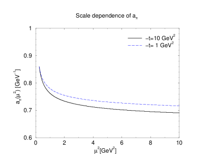
Figure 1: Scale dependence of the transverse size parameter $a_{\pi}$ with an initial value of $a_{\pi}=0.86$ GeV^-1 at $\mu_{0}^{2}=0.25$ GeV². As described in the text we have chosen $x=\langle x\rangle_{t}=0.75$. The two curves demonstrate the weak dependence on $t$.

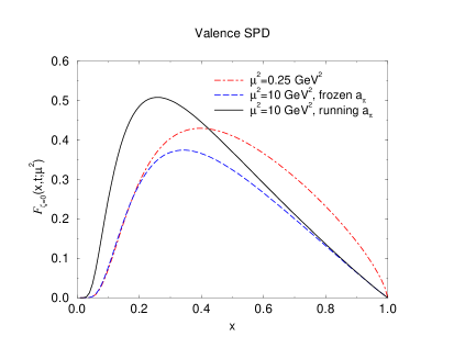
Figure 2: Evolution of the valence SPD (12) with constant and running $a_{\pi}$. We use the GRS parametrization of the forward valence distribution as stated in the text. At the starting scale $\mu_{0}^{2}=0.25$ GeV² both curves naturally coincide. The momentum transfer $-t$ is arbitrarily set to 1 GeV².

The scale dependence of the transverse size parameter is shown in Fig. 1. As can be expected $a_{\pi}$ depends only moderately on $\mu^{2}$ and the decrease is weakened with increasing scale. In Fig. 2 we have plotted the valence SPD (12) at two different scales. In order to see which quantitative effect the scale dependence of $a_{\pi}$ has on the SPD, we compare $\widetilde{\cal F}^{v}_{\zeta=0}(x,t;\mu^{2})$ with frozen (dashed line) and running $a_{\pi}$ (solid line), respectively, at $\mu^{2}=10$ GeV², where the scale dependence of the transverse size parameter causes a shift of the SPD towards smaller momentum fractions. At $\mu_{0}^{2}=0.25$ GeV² both curves coincide by definition (dot-dashed line).

At constant $a_{\pi}$ the parton distribution of the lowest Fock state which results from the LCWF (7) is scale independent. With increasing scale, however, one expects a damping of the parton distributions of lower Fock states since an increasing number of virtual quark-antiquark pairs and gluons is produced so that higher and higher Fock states become occupied. Quantitatively, this damping effect emerges through the Fock state probability in our approach. The Fock state probability of the $N$-th Fock state is defined by

$$P_{N}\equiv\sum_{\beta}\int[dx]_{N}[d^{2}{\bf k}_{\perp}]_{N}|\Psi_{N\beta}(x_{i},{\bf k}_{\perp i})|^{2}.$$ (18)

The running $a_{\pi}$ induces a scale dependent Fock state probability. As we have already discussed below Eq. (S0.Ex6) the normalization of the LCWF of the pion’s lowest Fock state is fixed so that for $P_{2}$ we have explicitly

$$P_{2}(\mu^{2})=2\pi^{2}\,f_{\pi}^{2}\,a_{\pi}^{2}(\mu^{2}),$$ (19)

which coincides with the well known value of $P_{2}=0.25$ at $\mu_{0}^{2}=0.25$ GeV² due to our choice of the initial value of $a_{\pi}$. As we can see immediately the Fock state probability of the lowest Fock state decreases with increasing scale since it is proportional to $a_{\pi}^{2}(\mu^{2})$. The value of $P_{2}$ at $\mu^{2}=100$ GeV² is reduced to about 0.14.

We can now write down the corresponding scale dependent valence quark distribution. Using the asymptotic form of the pion’s two-particle distribution amplitude in expression (9) we obtain

$$u_{v}^{(2)}(x;\mu^{2})=6\,P_{2}(\mu^{2})\,x\bar{x},$$ (20)

which is shown in Fig. 3 at two different scales, where we also compare with the GRS parametrization. The plot clearly shows the anticipated damping of the valence distribution with increasing scale. As discussed below Eq. (10) only a few Fock states contribute to the parton distribution at large $x$. We thus expect the valence distribution $u_{v}^{(2)}(x)$ of the lowest Fock state to approximate well the full valence distribution $u_{v}(x)$ at large $x$. With a fixed transverse size parameter, Fig. 3 shows that this expectation is not fulfilled at large scales for $x$ larger than 0.6 since $u_{v}(x)$ is shifted to smaller values of $x$ while $u_{v}^{(2)}(x)$ remains constant. We see that switching on the scale dependence of $a_{\pi}$ complies with our expectation provided that we take into account the theoretical and experimental uncertainties of the analysis of the Drell-Yan process $\pi^{-}p\to\mu^{+}\mu^{-}X$, from which the GRS parametrization of the valence distribution is extracted. In particular, for $x\raisebox{-4.0pt}{$\,\stackrel{{\scriptstyle\textstyle>}}{{\sim}}\,$}0.75$ the GRS valence distribution is less reliable since in that region the parametrization of the proton structure function, which is used as an input in the analysis, is an extrapolation. Our approach provides a clear improvement compared to the results of Ref. [16], where a constant transverse size parameter has been used and where thus a comparison of the full and the $N=2$ parton distributions has been possible only at low scale.

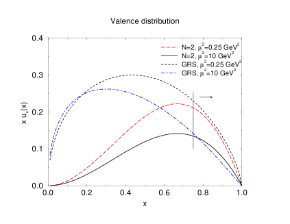
Figure 3: The scale dependent valence quark distribution (20) of the lowest $(N=2)$ Fock state (long dashed and solid lines) compared with the GRS parametrization (dashed and dot-dashed lines). As we discuss in the text to the right of the bar this parametrization becomes less reliable.

We will now consider the pion form factor, given by Eq. (3), as an application. Since the relevant scale in the overlap formula is given by the momentum transfer $t=-{\bf q}_{\perp}^{2}$ with ${\bf q}_{\perp}^{2}$ being the photon virtuality in a frame where the plus component of the momentum transfer vanishes, such that $\zeta=0$, it is natural to identify $\mu^{2}$ with $-t$. The result is shown in Fig. 4 (solid line). For comparison we also plot the form factor neglecting the evolution of both $q_{v}$ and $a_{\pi}$ (dashed line), and with fixed $a_{\pi}$ and running $q_{v}$ (dot-dashed line), respectively. The three curves show that the scale dependence of $a_{\pi}$ roughly compensates the evolution of the GRS valence distribution in the region 5 GeV${}^{2}\leq-t\leq 10$ GeV². For $-t<5$ GeV² the running $a_{\pi}$ even provides a slight enhancement of the theoretical prediction.

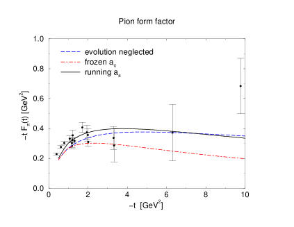
Figure 4: The pion form factor with constant and running $a_{\pi}$. The dashed line shows the case of constant $a_{\pi}=0.86$ GeV^-1, where we have also fixed the scale of the GRS valence distribution at 1 GeV². Data are taken from Ref. [17].

The authors of [6, 16] considered the contributions of the lowest Fock state only, without taking into account evolution effects of the transverse size parameter. Comparing their results with the dashed line of Fig. 4, where we have frozen the evolution scale of both the transverse size parameter and the valence distribution, we see that their prediction stays below ours. This has to be expected since we take into account the contributions of all Fock states.

The factorized GRS ansatz of Ref. [11] is essentially identical to our expression (12), again with a scale independent transverse size parameter and the GRS valence distribution at a fixed scale. Their corresponding prediction of the pion form factor is somewhat higher than ours. This is due to the fact that the parameter $\Lambda_{0}$ used in [11] corresponds to a transverse size parameter of $a_{\pi}\simeq 0.77$ GeV^-1, which is smaller than the value used in the present work.

The predictions of the hard contributions to $-t\,F_{\pi}(t)$ alone, ranging from 0.08 GeV² in [16] to about 0.16 GeV² in [19], obviously cannot account for the experimental data. We would like to point out that the sum of the hard part of Ref. [16] and our prediction of the soft part is in very good agreement with the new data between 0.6 and 1.6 GeV² presented in Ref. [20]. Note that in Ref. [21] strong cancellations between soft parts and hard parts of higher twist have been found, leaving small non-perturbative contributions.

To summarize, we have shown that the evolution equations for SPDs leads to a further constraint for phenomenological models of SPDs which are expressed through ordinary parton distributions. Starting from the generalized Drell-Yan formula, where the SPD for the $N$-th Fock state of the pion is written in terms of an overlap integral of $N$-particle light-cone wave functions, and specializing to the case of a zero skewedness parameter the SPD equals a Fock state parton distribution multiplied by an exponential function. Making further simplifications by assuming a common transverse size parameter for all Fock states we have obtained the full SPD, to which we have then applied the evolution equations. We have matched the generalized and ordinary DGLAP equations for the skewed and forward parton distributions, respectively, which has resulted in a constraint for the scale dependence of the transverse size parameter. This in turn has led to a scale dependent Fock state probability and valence quark distribution of the lowest Fock state of the pion. The application to the soft overlap contributions to the pion form factor has shown a slight enhancement of the theoretical prediction in the few GeV² region, which is in complete agreement with new data.

Finally, we would like to remark that LCWFs of the form (7), which are modified by an effective mass term, have also been discussed in the literature, see, for instance [8] and first Ref. of [19]. However, our discussion of the evolution effects shows that in principle one has to take into account the scale dependence of the effective mass as well, which would reduce the influence of a mass term in the LCWF with increasing scale.

Acknowledgements. I would like to thank Th. Feldmann and P. Kroll for stimulating discussions and critical comments. I have also benefited from discussions with A. P. Bakulev, R. Jakob, H. Huang and N. G. Stefanis. Moreover, I acknowledge a graduate grant of the Deutsche Forschungsgemeinschaft.

References

- [1] D. Müller, D. Robaschik, B. Geyer, F. M. Dittes and J. , Fortschr. Phys. 42, 101 (1994).
- [2] X. Ji, Phys. Rev. Lett. 78, 610 (1997); Phys. Rev. D 55, 7114 (1997).
- [3] A. V. Radyushkin, Phys. Lett. B 380, 417 (1996); Phys. Rev. D 56, 5524 (1997).
- [4] M. Diehl, Th. Feldmann, R. Jakob and P. Kroll, Eur. Phys. J. C 8, 409 (1999).
- [5] S. D. Drell and T.-M. Yan, Phys. Rev. Lett. 24, 181 (1970).
- [6] R. Jakob and P. Kroll, Phys. Lett. B 315, 463 (1993).
- [7] J. Bolz and P. Kroll, Z. Phys. A 356, 327 (1996).
- [8] S. J. Brodsky, T. Huang and G. P. Lepage, Particles and Fields 2, eds. Z. Capri and A.N. Kamal (Banff Summer Institute) p. 143 (1983).
- [9] A. V. Radyushkin, Phys. Rev. D 58, 114008 (1998).
- [10] A. V. Afanasev, hep-ph/9808291.
- [11] A. P. Bakulev, R. Ruskov, K. Goeke and N. G. Stefanis, Phys. Rev. D 62, 054018 (2000).
- [12] M. Miyama, S. Kumano, Comput. Phys. Commun. 94, 185 (1996).
-
[13]
I. V. Musatov and A. V. Radyushkin, Phys. Rev. D 56,
2713 (1997);
P. Kroll and M. Raulfs, Phys. Lett. B 387, 848, (1996). - [14] V. L. Chernyak and A. R. Zhitnitsky, Nucl. Phys. B 201, 492, (1982).
- [15] M. Glück, E. Reya, I. Schienbein, Eur. Phys. J. C 10, 313 (1999).
- [16] R. Jakob, P. Kroll and M. Raulfs, J. Phys. G 22, 45 (1996).
- [17] C. J. Bebek et al. Phys. Rev. D 17, 1693 (1978).
- [18] S. J. Brodsky, hep-ph/9908456.
-
[19]
N. G. Stefanis, W. Schroers and H.-Ch. Kim, hep-ph/0005218;
Phys. Lett. B 449, 299 (1999). - [20] J. Volmer et al., nucl-ex/0010009.
- [21] V. M. Braun, A. Khodjamirian and M. Maul, Phys. Rev. D 61, 073004 (2000).