DESY 00–105
SNUTP 00–018

Measuring MSSM CP–violating Phases through Spin
Correlated Supersymmetric Tri–lepton Signatures
at the Tevatron
S.Y. Choi1, M. Guchait2, H.S. Song3 and W.Y. Song3


1Department of Physics, Chonbuk National University, Chonju 561–756, Korea
2Deutsches Elektronen–Synchrotron DESY, D-22603 Hamburg, Germany
3CTP and Department of Physics, Seoul National University, Seoul 151-742, Korea


Abstract

We provide a detailed analysis of the supersymmetric tri–lepton signals for sparticle searches at the Tevatron in the minimal supersymmetric standard model with general CP–violating phases but without flavor mixing among sfermions of different generation. The stringent experimental constraints on the CP–violating phases from the electron and neutron electric dipole moments are included in the analysis for two exemplary scenarios of the SUSY parameters; one with decoupled first two generation sfermions and the other with non–decoupled sfermions. In both scenarios, the production cross section and the branching fractions of the leptonic chargino and neutralino decays are sensitive to CP–violating phases. The production–decay spin correlations lead to several non–trivial CP–even observables such as the lepton invariant mass distribution and the lepton angular distribution, and several interesting T–odd (CP–odd) momentum triple products. The possibility of measuring the CP–violating phases directly through those T–odd observables is investigated in detail.

1 Introduction

Supersymmetry is the currently best motivated extension of the Standard Model (SM) of particle physics which allows to stabilize the gauge hierarchy without getting into conflict with electroweak precision data. Among all possible supersymmetric theories, the Minimal Supersymmetric Standard Model (MSSM) occupies a special position. It is not only the simplest, i.e. most economical, potentially realistic supersymmetric field theory, but it also has just the right particle content to allow for the unification of all gauge interactions [1].

The R–parity preserving MSSM [2] as a softly–broken SUSY model contains in general more than one–hundred independent physical parameters including about forty–five CP–violating physical phases [3] in the Lagrangian. The CP–violating phases, if they are large, can give a significant impact on not only various CP–odd observables but also the CP–even quantities such as sparticle masses [4], production cross sections, branching fractions [5], LSP relic density [6], Higgs boson masses and couplings [7], CP violation in the $B$ and $K$ systems [8], and so on.

The most stringent (indirect) constraints [9] on the MSSM CP–violating phases come from the precise measurements of the electron and neutron electric dipole moments (EDM), but the indirect EDM constraints depend strongly on the assumptions taken in the analysis without any a priori justifications. Relaxing the rather stringent assumptions, several recent works [10, 11] have shown that the constraints could be evaded without suppressing the CP–violating phases of the theory. One option [11] is to make the first two generations of scalar fermions very heavy so that one–loop EDM constraints are automatically evaded while keeping the third-generation sfermions relatively light to preserve naturalness. This case can be naturally explained by the so–called effective SUSY models [12] where de–couplings of the first and second generation sfermions are invoked to solve the SUSY FCNC and CP problems without spoiling naturalness. Another possibility is that various SUSY parameters are arranged [10] to lead to partial cancellations among their contributions to the electron and neutron EDMs without taking very large sfermion masses. Consequently, it is not yet clear at all whether the CP–violating phases of the MSSM are small or not. Once supersymmetric particles are discovered at colliders, it will be therefore of great importance to directly measure the CP–violating phases as well as the other real parameters of the supersymmetric Lagrangian.

In this paper we illustrate how the presence of the CP–violating phases affects observables which can be measured in the classical reaction $p\bar{p}\rightarrow\tilde{\chi}^{\pm}_{1}\tilde{\chi}^{0}_{2}$ with subsequent decays $\tilde{\chi}^{\pm}_{1}\rightarrow\tilde{\chi}^{0}_{1}\,\ell^{\pm}\bar{\nu}_{\ell}$ and $\tilde{\chi}^{0}_{2}\rightarrow\tilde{\chi}^{0}_{1}\,\ell^{\prime+}\ell^{\prime-}$ $(\ell,\,\ell^{\prime}=e,\,\mu)$ when the lightest neutralino $\tilde{\chi}^{0}_{1}$ is the lightest supersymmetric particle (LSP). Such tri–lepton signatures have been investigated in several CDF and D0 analyses at the Tevatron based on the models with only real SUSY parameters. That is to say, most of the works [13] have been done under the assumption that all the couplings are related at the grand unification or Planck scale and they are real. In the light of the possibility of large CP–violating phases, we investigate systematically the impact of the CP–violating phases on the SUSY tri–lepton signatures at the Tevatron, including the constraints on the phases imposed by the electron and neutron EDMs and taking into account the full spin/angular correlations between the production and the leptonic decays of the associated chargino and neutralino pair.

The paper is organized as follows. In Sect. 2 we describe the chargino, neutralino and flavor–preserving sfermion mixing phenomena on the most general footing and identify all the relevant physical CP–violating phases. Section 3 is devoted to the detailed discussion of the constraints by the electron and neutron EDM measurements on the CP–violating phases. In Sect. 4 we present in detail the formalism to describe the associated production of the chargino $\tilde{\chi}^{\pm}_{1}$ and the neutralino $\tilde{\chi}^{0}_{2}$ in $p\bar{p}$ collisions at the Tevatron; production helicity amplitudes, chargino and neutralino mass spectra, and chargino and neutralino polarization vectors. Section 5 is devoted to the detailed description of the decay modes of the chargino $\tilde{\chi}^{\pm}_{1}$ and the neutralino $\tilde{\chi}^{0}_{2}$ and their branching fractions. In Sect. 6 after explaining the method of obtaining the fully spin–correlated distributions of the associated production and decays of the chargino and neutralino, we investigate in detail the impact of the CP–violating phases on various physical observables such as the total rate of the tri–lepton signatures, the dilepton invariant mass distributions, the lepton angle distribution as well as the CP–odd triple products of three proton and/or lepton momenta. Finally, we summarize our findings and conclude in Sect. 7.

2 Supersymmetric Flavor Conserving Mixing

The existence of the non–trivial MSSM CP–violating phases is due to SUSY breakdown, so that the CP–violating phases appear in the soft–breaking parameters and the mixing among sparticles due to the electroweak gauge symmetry breaking. As a whole, the MSSM has three well–known sources of CP violation. The first is related to the two Higgs–boson doublets present in the model as both the $\mu$ parameter in the superpotential and the soft breaking parameter $B$ can be complex. We denote the phases of $\mu$ and $B$ by $\Phi_{\mu}$ and $\Phi_{B}$, respectively. Secondly, there are three more phases $\{\Phi_{1},\Phi_{2},\Phi_{3}\}$ related to the complex U(1)Y, SU(2)L and SU(3)C gauginos masses. Finally, most of the other CP–violating phases originate from the flavor sector of the MSSM Lagrangian, either in the scalar soft mass matrices or in the trilinear matrices.

The sfermion mass matrices are Hermitian so that only off-diagonal terms can be complex, but the trilinear matrices are in general $3\times 3$ matrices allowing for the complex diagonal entries. The effects of the phases associated with the off-diagonal terms on experimental observables are strongly suppressed by the same mechanism required to suppress the flavor changing neutral current effects. Therefore, we neglect these flavor–changing CP–violating phases in the present work assuming that all the scalar soft mass matrices and trilinear parameters are flavor diagonal and the complex trilinear terms $A_{f}$ with its phase $\Phi_{A_{f}}$ are proportional to the corresponding fermion Yukawa couplings. Consequently, the gaugino masses $M_{1}$, $M_{2}$, $M_{3}$ and the higgsino mass parameter $\mu$ as well as the trilinear parameters $A_{f}$ can be complex in the CP–noninvariant theories. However, reparameterising the fields one can take $M_{2}$ to be real and positive without any loss of generality and all other parameter choices are related to the specific choice by an appropriate R transformation.

Neglecting flavor mixing among sfermions, the sfermion mass matrix squared is given by

$\displaystyle{\cal M}^{2}_{\tilde{f}}=\left(\begin{array}[]{cc}\tilde{m}^{2}_{\tilde{f}_{L}}+m^{2}_{f}+D_{f_{L}}&m^{2}_{\tilde{f}LR}\\[5.69054pt] m^{2*}_{\tilde{f}LR}&\tilde{m}^{2}_{\tilde{f}_{R}}+m^{2}_{f}+D_{\bar{f}_{R}}\end{array}\right).$ (3)

where the mixing term $m^{2}_{\tilde{f}LR}$, and $D_{f_{L}}$ and $D_{\bar{f}_{R}}$ are:

$\displaystyle m^{2}_{\tilde{f}LR}=-m_{f}\left(A^{*}_{f}+\mu\tan\beta/\cot\beta\right)\ \ {\rm for}~{}~{}f=d,e/u\,,$
$\displaystyle D_{f_{L}}=m_{Z}^{2}\cos 2\beta\left(T^{f}_{3L}-Q_{f}\,s^{2}_{W}\right)\,,\qquad D_{\bar{f}_{R}}=m_{Z}^{2}\cos 2\beta\,Q_{f}\,s^{2}_{W}\,.$ (4)

The first term of each diagonal element is the soft scalar mass term evaluated at the weak scale, and the second is the mass squared of the corresponding sfermion mass, and the last one is the so-called $D$ term of the MSSM superpotential. The trilinear term $A_{f}$ causing the left–right mixing is due to the soft–breaking Yukawa–type interaction, and $\mu$ is the complex supersymmetric higgsino mass parameter and $\tan\beta$ is the ratio $v_{2}/v_{1}$ of the vacuum expectation values of the two neutral Higgs fields which break the electroweak gauge symmetry. The sfermion mass eigenvalues and eigenstates can be obtained by diagonalizing the above mass matrix with a unitary matrix $U_{\tilde{f}}$ such that $U_{\tilde{f}}^{\dagger}\,{\cal M}^{2}_{\tilde{f}}\,U_{\tilde{f}}={\rm diag}(m^{2}_{\tilde{f}_{1}},m^{2}_{\tilde{f}_{2}})$. We parameterize $U_{\tilde{f}}$ as

$\displaystyle U_{\tilde{f}}=\left(\begin{array}[]{cc}\cos\theta_{f}&-\sin\theta_{f}\,{\rm e}^{-i\phi_{f}}\\[2.84526pt] \sin\theta_{f}\,{\rm e}^{i\phi_{f}}&\cos\theta_{f}\end{array}\right),$ (7)

where $\phi_{f}={\rm arg}[-m_{f}\,(A_{f}+\mu^{*}\tan\beta)]$, $0\leq\theta_{f}\leq\pi$ and $-\pi/2\leq\phi_{f}\leq\pi/2$ without any loss of generality.

In the MSSM, the spin–1/2 supersymmetric partners of the $W^{\pm}$ boson and the charged Higgs boson, $\tilde{W}^{\pm}$ and $\tilde{H}^{\pm}$, respectively, mix to form the chargino mass eigenstates $\tilde{\chi}^{\pm}_{1,2}$. The chargino mass matrix dictating this mixing is given in the $\{\tilde{W}^{-},\tilde{H}^{-}\}$ basis by

$\displaystyle{\cal M}_{C}=\left(\begin{array}[]{cc}M_{2}&\sqrt{2}\,m_{W}\,c_{\beta}\\[2.84526pt] \sqrt{2}\,m_{W}\,s_{\beta}&|\mu|\,{\rm e}^{i\Phi_{\mu}}\end{array}\right),$ (10)

which is built up by the fundamental SUSY parameters; the SU(2)L gaugino mass $M_{2}$, the modulus and phase of $\mu$, $s_{\beta}\equiv\sin\beta$ and $c_{\beta}\equiv\cos\beta$. Since the chargino mass matrix ${\cal M}_{C}$ is not symmetric, two different unitary matrices acting on the left– and right–chiral $(\tilde{W},\tilde{H})$ states are needed to diagonalize the mass matrix ${\cal M}_{C}$:

$\displaystyle U_{L,R}\left(\begin{array}[]{cc}\tilde{W}^{-}\\ \tilde{H}^{-}\end{array}\right)_{L,R}=\left(\begin{array}[]{cc}\tilde{\chi}^{-}_{1}\\ \tilde{\chi}^{-}_{1}\end{array}\right)_{L,R},$ (15)

so that $U_{R}{\cal M}_{C}U^{\dagger}_{L}={\rm diag}\,(m_{\tilde{\chi}^{\pm}_{1}},m_{\tilde{\chi}^{\pm}_{2}})$ with the ordering of $m_{\tilde{\chi}^{\pm}_{1}}\leq m_{\tilde{\chi}^{\pm}_{2}}$ as a convention.

The supersymmetric spin–1/2 partners of the neutral U(1)Y and SU(2)L gauge bosons, $\tilde{B}$ and $\tilde{W}^{3}$, respectively, mix with the supersymmetric fermionic partners of the neutral Higgs bosons, $\tilde{H}^{0}_{1}$ and $\tilde{H}^{0}_{2}$, to form mass eigenstates. The four physical mass eigenstates $\tilde{\chi}^{0}_{i}$ ($i=1$ to 4), called neutralinos, are obtained by diagonalizing the $4\times 4$ neutralino mass matrix

$\displaystyle{\cal M}_{N}=\left(\begin{array}[]{cccc}|M_{1}|\,{\rm e}^{i\Phi_{1}}&0&-m_{Z}c_{\beta}s_{W}&m_{Z}s_{\beta}s_{W}\\ 0&M_{2}&m_{Z}c_{\beta}c_{W}&-m_{Z}s_{\beta}c_{W}\\[1.42262pt] -m_{Z}c_{\beta}s_{W}&m_{Z}c_{\beta}s_{W}&0&-|\mu|\,{\rm e}^{i\Phi_{\mu}}\\ m_{Z}s_{\beta}s_{W}&-m_{Z}s_{\beta}c_{W}&-|\mu|\,{\rm e}^{i\Phi_{\mu}}&0\end{array}\right),$ (20)

where $s_{W}\equiv\sin\theta_{W}$ and $c_{W}\equiv\cos\theta_{W}$. Since the neutralino mass matrix ${\cal M}_{N}$ is a complex and symmetric so that it can be diagonalized by a single unitary matrix $N$ as $N^{*}{\cal M}_{N}N^{\dagger}={\rm diag}\,(m_{\tilde{\chi}^{0}_{1}},m_{\tilde{\chi}^{0}_{2}},m_{\tilde{\chi}^{0}_{3}},m_{\tilde{\chi}^{0}_{4}})$ with the ordering of $m_{\tilde{\chi}^{0}_{1}}\leq m_{\tilde{\chi}^{0}_{2}}\leq m_{\tilde{\chi}^{0}_{3}}\leq m_{\tilde{\chi}^{0}_{4}}$. On the other hand, the gluinos, the spin–1/2 partners of gluons, do not mix among themselves and involve only a single complex phase $\Phi_{3}$.

To recapitulate, we have in total twelve non–trivial CP–violating phases; two phases $\{\Phi_{1},\Phi_{3}\}$ from the gaugino sector, one phase $\Phi_{\mu}$ from the higgsino sector, and nine phases $\Phi_{A_{f}}$ for the nine sfermion flavors.

3 Electron and Neutron Electric Dipole Moments

The electric dipole interaction of a spin–1/2 charged particle $f$ with an electromagnetic field is described in a model–independent way by the 5–dimensional effective Lagrangian

$\displaystyle{\cal L}_{\rm EDM}=-\frac{i}{2}\,d_{f}\,\bar{f}\sigma^{\mu\nu}\gamma_{5}f\,F_{\mu\nu}.$ (21)

In theories with CP–violating interactions, the electric dipole moment $d_{f}$ receives contributions from loop diagrams. In the case of the electron EDM the chargino–sneutrino and neutralino–slepton loops contribute whereas in the quark case the chargino–squark, neutralino–squark and gluino–squark loops are involved (See Fig. 1). Recently, one–loop chromoelectric dipole moment (CEDM) contributions have been studied in Ref. [10] and found to be comparable to the EDM ones. In addition, there is a significant contribution to the neutron EDM through the so–called Weinberg’s three–gluon dimension–six operator [10, 14]. Therefore, for the CEDMs of quarks we include the chargino–squark, neutralino-squark and gluino–squark loops, where the gluonic dimension–six operator gets contributions from the loop containing top (s)quark and gluinos. The quark CEDM is then defined as the coefficient $\hat{d}_{q}$ in the 5-dimensional effective Lagrangian

$\displaystyle{\cal L}_{\rm CEDM}=-\frac{i}{2}\,\hat{d}_{q}\,\bar{q}\sigma^{\mu\nu}\gamma_{5}T^{a}q\,G^{a}_{\mu\nu}\,,$ (22)

where the indices $a$ ($=1$ to 8) denote the gluons and $T^{a}$ are the SU(3)C generators. And, the gluonic dimension-six operator is given by

$\displaystyle{\cal L}_{\rm 3G}=-\frac{1}{6}\,d_{G}f_{abc}\,\epsilon^{\mu\nu\lambda\sigma}\,G^{a}_{\mu\rho}G^{b\rho}_{\nu}G^{c}_{\lambda\sigma}\,.$ (23)

The various SUSY contributions to the fermion EDM are illustrated in Fig. 1; the diagram (a) denotes the chargino, neutralino, and gluino loops where the dashed line of each loop is for a scalar fermion mass eigenstate corresponding to the fermion, and the diagram (b) is for the effective 3–gluon operator. Both of them contribute to the coefficients $d_{f}$ and $\hat{d}_{q}$ depending on whether a photon or a gluon is radiated off the loop. These contributions can be calculated at the electroweak scale since a typical SUSY scale in most SUSY models is of the same order of magnitude as the electroweak scale.

In the following we enumerate all the SUSY contributions to the first–generation fermion EDMs. The chargino–loop contributions are determined by the Lagrangian

$\displaystyle{\cal L}_{\tilde{\chi}^{\pm}f\tilde{f}^{\prime}}$ $\displaystyle=$ $\displaystyle\frac{e}{s_{W}}\sum_{i=1}^{2}\sum_{j=1}^{2}\bigg{\{}\bar{e}\left[Y_{e}U^{*}_{Lj2}\delta_{i1}P_{L}-U^{*}_{Rj1}P_{R}\delta_{i1}\right]\tilde{\chi}^{-}_{j}\tilde{\nu}_{i}$
$\displaystyle\hskip 51.21504pt+\bar{d}\left[Y_{d}U^{*}_{Lj2}U_{\tilde{u}1i}P_{L}+(Y_{u}U^{*}_{Rj2}U_{\tilde{u}2i}-U^{*}_{Rj1}U_{\tilde{u}1i})P_{R}\right]\tilde{\chi}^{-}_{j}\tilde{u}_{i}$
$\displaystyle\hskip 51.21504pt+\bar{u}\left[Y_{u}U_{Rj2}U_{\tilde{d}1i}P_{L}+(Y_{d}U_{Lj2}U_{\tilde{d}2i}-U_{Lj1}U_{\tilde{d}1i})P_{R}\right]\tilde{\chi}^{+}_{j}\tilde{d}_{i}\bigg{\}}+{\rm H.c.},$

describing the $\tilde{\chi}^{\pm}$ $f$ $\tilde{f}^{\prime}$ interactions for the first generation sfermions without flavor mixing. Here $P_{L,R}=(1\mp\gamma_{5})/2$ and $\{Y_{e},Y_{d},Y_{u}\}$ are the Yukawa couplings:

$\displaystyle Y_{e}=\frac{m_{e}}{\sqrt{2}m_{W}\,c_{\beta}}\,,\ \ Y_{d}=\frac{m_{d}}{\sqrt{2}m_{W}\,c_{\beta}}\,,\ \ Y_{u}=\frac{m_{u}}{\sqrt{2}m_{W}\,s_{\beta}}\,.$ (25)

One can readily find out that the interactions of the charginos with a fermion and a sfermion contribute to the EDM of the fermion $f$ as

$\displaystyle d_{f}^{\tilde{\chi}^{-}}=-\frac{e\alpha}{4\pi s^{2}_{W}}\sum_{i=1}^{2}\sum_{j=1}^{2}\frac{m_{{\chi}^{-}_{j}}}{m^{2}_{\tilde{f}_{i}}}~{}\Im{\rm m}(\Delta^{f{\tilde{\chi}^{-}}}_{ij})\left[Q_{\tilde{f}}\,B\!\left(\frac{m^{2}_{{\chi}^{-}_{j}}}{m^{2}_{\tilde{f}_{i}}}\right)+(Q_{f}-Q_{\tilde{f}})\,A\!\left(\frac{m^{2}_{{\chi}^{-}_{j}}}{m^{2}_{\tilde{f}_{i}}}\right)\right],$ (26)

where the dimensionless functions $A(r)$ and $B(r)$ are defined as

$\displaystyle A(r)=\frac{1}{2(1-r)^{2}}\left[3-r+2\,\left(\frac{\ln r}{1-r}\right)\right]\,,\ \ B(r)=\frac{1}{2(1-r)^{2}}\left[1+r+2\,\left(\frac{r\ln r}{1-r}\right)\right]\,,$ (27)

and

$\displaystyle\begin{array}[]{ll}\Delta^{e{\tilde{\chi}^{-}}}_{ij}=Y_{e}\,U^{*}_{Lj2}U_{Rj1}\delta_{i1}&\ \ (Q_{f}=Q_{e},\,Q_{\tilde{f}}=0,\,m_{\tilde{f}_{i}}=m_{\tilde{\nu}_{e}}),\\[2.84526pt] \Delta^{u{\tilde{\chi}^{-}}}_{ij}=Y_{u}\,U_{Rj2}U^{\tilde{d}}_{1i}\left[U^{*}_{Lj1}U^{\tilde{d}*}_{1i}-Y_{d}\,U^{*}_{Lj2}U^{\tilde{d}*}_{2i}\right]&\ \ (Q_{f}=Q_{u},\,Q_{\tilde{f}}=Q_{\tilde{d}},\,m_{\tilde{f}_{i}}=m_{\tilde{u}_{i}}),\\[2.84526pt] \Delta^{d{\tilde{\chi}^{-}}}_{ij}=Y_{d}\,U_{Lj2}U^{\tilde{u}}_{1i}\left[U^{*}_{Rj1}U^{\tilde{u}*}_{1i}-Y_{u}\,U^{*}_{Rj2}U^{\tilde{u}*}_{2i}\right]&\ \ (Q_{f}=Q_{d},\,Q_{\tilde{f}}=Q_{\tilde{u}},\,m_{\tilde{f}_{i}}=m_{\tilde{d}_{i}}).\end{array}$ (31)

On the other hand, the chargino contributions to the CEDM of the quark $q$ are given by

$\displaystyle\hat{d}_{q}^{\tilde{\chi}^{-}}=-\frac{g_{s}\alpha}{4\pi s^{2}_{W}}\sum_{i=1}^{2}\sum_{j=1}^{2}\frac{m_{{\chi}^{-}_{j}}}{m^{2}_{\tilde{q}_{i}}}~{}\Im{\rm m}(\Delta^{q{\tilde{\chi}^{-}}}_{ij})\,B\!\left(\frac{m^{2}_{{\chi}^{-}_{j}}}{m^{2}_{\tilde{q}_{i}}}\right).$ (32)

Secondly, the neutralino–loop contributions to the EDM of a fermion $f$ are determined by the Lagrangian describing the most general $\tilde{\chi}^{0}$ $f$ $\tilde{f}$ interactions,

$\displaystyle{\cal L}_{\tilde{\chi}^{0}f\tilde{f}}=-\frac{e}{\sqrt{2}s_{W}}\sum_{i=1}^{2}\sum_{j=1}^{4}\bar{f}\left[B^{f_{L}}_{ij}P_{L}+B^{f_{R}}_{ij}P_{R}\right]\tilde{\chi}^{0}_{j}\tilde{f}_{i}+{\rm H.c.},$ (33)

where the couplings $B^{f_{L}}_{ij}$ and $B^{f_{R}}_{ij}$ are given by

$\displaystyle B^{f_{L}}_{ij}=\sqrt{2}Y_{f}N^{*}_{jh}U_{\tilde{f}1i}-2Q_{f}N^{*}_{j1}\tan\theta_{W}U_{\tilde{f}2i}\,,$
$\displaystyle B^{f_{R}}_{ij}=2\left[T^{f}_{3}N_{j2}+(Q_{f}-T^{f}_{3})\tan\theta_{W}N_{j1}\right]U_{\tilde{f}1i}+\sqrt{2}Y_{f}N_{jh}U_{\tilde{f}2i}\,,$ (34)

with $h=3$ for $f$ = $d,e$ and $h$ = 4 for $f$ = $u$, respectively. The neutralino contributions to the EDM of a fermion $f$ is then given by

$\displaystyle d_{f}^{\tilde{\chi}^{0}}=\frac{e\alpha}{8\pi s^{2}_{W}}Q_{f}\sum_{i=1}^{2}\sum_{j=1}^{4}\left\{\frac{m_{\tilde{\chi}^{0}_{j}}}{m^{2}_{\tilde{f}_{i}}}\,\Im{\rm m}\left[B^{fL}_{ij}B^{fR*}_{ij}\right]B\!\left(\frac{m^{2}_{\tilde{\chi}^{\pm}_{j}}}{m^{2}_{\tilde{f}_{i}}}\right)\right\},$ (35)

and the neutralino contributions to the CEDM $\hat{d}_{q}^{\tilde{\chi}^{0}}$ of the quark $q$ can be obtained by simply replacing $e$ by $g_{s}$ and $Q_{f}$ by unity in eq. (35).

Thirdly, the gluino–loop contributions to the fermion EDMs are determined by the Lagrangian describing the most general $\tilde{g}$ $q$ $\tilde{q}$ interactions

$\displaystyle{\cal L}_{\tilde{g}q\tilde{q}}=\sqrt{2}g_{s}(T^{a})_{lm}\sum_{i=u,d}\left(e^{-i\Phi_{3}/2}\,\bar{q}^{l}_{i}P_{L}\tilde{g}^{a}\tilde{q}^{m}_{iR}+e^{i\Phi_{3}/2}\,\bar{q}^{l}_{i}P_{R}\tilde{g}^{a}\tilde{q}^{m}_{iL}\right)+{\rm H.c.}\,,$ (36)

where the indices $l$ and $m$ ($=1$ to $3$) are for the color of quarks and squarks, the index $a$ ($=1$ to 8) is for the color of a gluino $\tilde{g}^{a}$, and the 3$\times$3 matrix $T_{a}$ is a SU(3)C generator. The gluino contributions to the coefficients $d_{q}$ and $\hat{d}_{q}$ are given by

$\displaystyle d_{q}^{\tilde{g}}=-\frac{2e\alpha_{s}}{3\pi}Q_{q}\sum_{i=1}^{2}\frac{m^{2}_{g}}{m^{2}_{\tilde{q}_{i}}}\Im{\rm m}(e^{-i\Phi_{3}}U_{\tilde{q}2i}U^{*}_{\tilde{q}1i})\,B(x)\,,$
$\displaystyle\hat{d}_{q}^{\tilde{g}}=\frac{g_{s}\alpha_{s}}{4\pi}\sum_{i=1}^{2}\frac{m^{2}_{g}}{m^{2}_{\tilde{q}_{i}}}\Im{\rm m}(e^{-i\Phi_{3}}U_{\tilde{q}2i}U^{*}_{\tilde{q}1i})\,C(x)\,,$ (37)

with the dimensionless function $C(x)$ defined as

$\displaystyle C(r)=-3A(r)+\frac{B(r)}{3}\,.$ (38)

Finally,  the leading nontrivial MSSM contribution to the CP–odd three–gluon term $d_{G}$ is given by a two–loop diagram involving the top, top squarks and gluinos [10]:

$\displaystyle d_{G}$ $\displaystyle=$ $\displaystyle\frac{3g_{s}\alpha_{s}^{2}}{16\pi^{2}}\frac{m_{t}(m^{2}_{\tilde{t}_{2}}-m^{2}_{\tilde{t}_{1}})}{m^{5}_{\tilde{g}}}\,\Im{\rm m}(e^{-i\Phi_{3}}U^{\tilde{t}}_{22}U^{\tilde{t}*}_{12})\,H(x_{1},x_{2},x_{3})\,,$ (39)

where $x_{1}=m^{2}_{\tilde{t}_{1}}/m^{2}_{\tilde{g}}$, $x_{2}=m^{2}_{\tilde{t}_{2}}/m^{2}_{\tilde{g}}$, $x_{3}=m^{2}_{t^{2}}/m^{2}_{\tilde{g}}$, and the two–loop function $H$ is given by the three–fold integral

$\displaystyle H(z_{1},z_{2},z_{3})=\frac{1}{2}\int_{0}^{1}{\rm d}x\int_{0}^{1}{\rm d}u\int_{0}^{1}{\rm d}y\,x(1-x)u\,\frac{N_{1}N_{2}}{D^{4}},$ (40)

where the explicit forms of the $N_{1}$, $N_{2}$ and $D$ are given by

$\displaystyle N_{1}$ $\displaystyle=$ $\displaystyle u(1-x)+z_{3}x(1-x)(1-u)-2ux[z_{1}y+z_{2}(1-y)]\,,$
$\displaystyle N_{2}$ $\displaystyle=$ $\displaystyle(1-x)^{2}(1-u)^{2}+u^{2}-\frac{1}{9}x^{2}(1-u)^{2}\,,$
$\displaystyle D$ $\displaystyle=$ $\displaystyle u(1-x)+z_{3}x(1-x)(1-u)+ux[z_{1}y+z_{2}(1-y)]\,.$

Having defined the contributions from the individual Feynman diagrams, the total EDM of electron is given simply by the sum of the chargino and neutralino contributions:

$$d_{e}=d_{e}^{\tilde{\chi}^{+}}+d_{e}^{\tilde{\chi}^{0}}\,.$$ (41)

In principle, the Kobayashi–Maskawa (KM) CP phase in the SM can contribute to the electron EDM, but it turns out to be effective only at the three–loop level so that the contribution is too small to be considered.

On the other hand, the EDM of the neutron, a composite particles of quarks and gluons, can be obtained from the EDMs of the constituent quarks and gluons. The quark EDM evaluated at the electro–weak scale must be evolved down to the hadronic scale via renormalization group equation (RGE). Generally, the prescription based on the effective chiral quark theory given in Ref. [15], are used to calculate the neutron EDM from the quark EDMs. According to the model, the neutron EDM is given by

$\displaystyle d_{n}=\frac{4}{3}\,d_{d}-\frac{1}{3}\,d_{u}.$ (42)

In order to evaluate the numerical value of each individual quark EDM from the effects of the EDM operators given in eqs. (32), (35), (37) and (39) we use the so–called “naive dimensional analysis” as proposed in Ref. [15]. The explicit form of the quark EDMs are then given by the contributions of all quark and gluon operators (to leading order in $\alpha_{s}$) with the proper dimensional re–scalings as

$\displaystyle d_{q}=\eta^{E}(d_{q}^{\tilde{\chi}^{+}}+d_{q}^{\tilde{\chi}^{0}}+d_{q}^{\tilde{g}})+\eta^{C}\frac{e}{4\pi}(\hat{d}_{q}^{\tilde{\chi}^{+}}+\hat{d}_{q}^{\tilde{\chi}^{0}}+\hat{d}_{q}^{\tilde{g}})+\eta^{G}\,\frac{e\Lambda_{SB}}{4\pi}d_{G}\,,$ (43)

where $\eta^{E}$, $\eta^{C}$, and $\eta^{G}$ are the QCD correction factors due to the renormalization group equations, whereas $\Lambda_{SB}$ is the scale of chiral symmetry breaking in QCD; we use $\eta^{E}=1.53$ [16], $\eta^{C}\simeq\eta^{G}\simeq 3.4$ [10], and $\Lambda_{SB}\simeq 1.19$ GeV [15].

Although flavor mixing is neglected, there are still sixteen real parameters and seven CP–violating phases: $\{\tan\beta,\,|M_{1}|,\,M_{2},\,|M_{3}|,\,|\mu|,\,m_{\tilde{f}_{L}},\,m_{\tilde{f}_{R}},\,|A_{f}|\}$ and $\{\Phi_{1},\Phi_{3},\Phi_{\mu},\Phi_{A_{f}}\}$ for $f=e,u,d,t$ where the SU(2) relation $m_{\tilde{u}_{L}}=m_{\tilde{d}_{L}}$ is taken into account. So, any reasonable quantitative understanding of the general features of the SUSY contributions to the electron and neutron EDMs requires us to make a few appropriate assumptions on the SUSY parameters without spoiling their qualitative aspects; (i) we take a universal soft–breaking selectron mass $m_{\tilde{e}}$ and squark mass $m_{\tilde{q}}$ for the first–generation left– and right–handed selectrons and squarks, respectively, and $m_{\tilde{t}}$ for the left– and right–handed top squarks; (ii) the gaugino mass unification condition is assumed only for the modulus of the U(1)Y and SU(2)L gaugino mass parameters, i.e. $|M_{1}|=\frac{5}{3}\tan^{2}\theta_{W}\,M_{2}\approx 0.5\,M_{2}$ and the absolute value of the gluino mass, $|M_{3}|$, is taken to be 500 GeV; (iii) we take $|A_{f}|$ to be 1 TeV for any sfermion $\tilde{f}$ such that the EDM constraints are satisfied. We should be very careful in choosing the value of $\tan\beta$ which has very significant effect to many SUSY processes. According to the recent calculation for the Barr–Zee–type two–loop contributions to the fermion EDMs by Chang, Keung and Pilaftsis [17], the bottom squark contributions are very much enhanced for large $\tan\beta$ [18] so that their contributions cannot be neglected. Therefore, for large $\tan\beta$ we are forced to introduce additional CP–violating phases in our analysis related with the sparticles of the third generation. Moreover, a large $\tan\beta$ yields a large tau slepton left–right mixing and the Higgs–exchange diagrams in the decays of the neutralinos into tau or bottom pairs cannot be neglected due to the enhanced Yukawa couplings of third generation. On the contrary, the value of $\tan\beta$ less than about 2 has been already ruled out by negative results in the Higgs search experiments at LEP II [19] based on the minimal supergravity scenario with real couplings. However, this experimental constraint on $\tan\beta$ may be loosened in CP noninvariant theories. Putting off the detailed investigation related with the $\tan\beta$ dependence of the EDMs, the associated production of chargino and neutralino, and their branching ratios, we simply take $\tan\beta=3$ in the present analysis, for which the tau-slepton contributions can be treated on the same footing as the other slepton contributions.

With these assumptions on the SUSY parameters given in the previous paragraph, the electron and neutron EDMs are determined by just five real parameters and seven remaining CP–violating phases:

$\displaystyle\{M_{2},\,|\mu|,\,m_{\tilde{e}},\,m_{\tilde{q}},\,m_{\tilde{t}}\,\,;\,\,\Phi_{1},\,\Phi_{\mu},\,\Phi_{3},\,\Phi_{A_{e}},\,\Phi_{A_{q}},\,\Phi_{A_{t}}\}\,,$ (44)

with $q=u,\,d$. Let us take two extreme scenarios for allowing relatively large CP–violating phases without violating the EDM constraints. Firstly, based on the so-called effective SUSY model [12] we decouple the first and second generation sfermions by rendering them very heavy without violating naturalness by maintaining the third generation sfermions to be light and taking $M_{2}$ and $|\mu|$ relatively small:

$\displaystyle{\cal S}1:\ \ \{M_{2}=100\,{\rm GeV},\,\,|\mu|=200\,{\rm GeV},\,\,m_{\tilde{f}}=10\,{\rm TeV},\,\,m_{\tilde{t}}=500\,{\rm GeV}\}\,,$ (45)

In this scenario, the sfermion masses $m_{\tilde{f}}$ $(f=e,u,d)$ are large enough to suppress the sfermion contributions to the electron and neutron EDMs completely. As a result, the present EDM bounds [20] on the electron and neutron EDMs

$\displaystyle|d_{e}|\leq 4.3\times 10^{-27}\,e\cdot{\rm cm}\,,\qquad|d_{n}|\leq 1.1\times 10^{-25}\,e\cdot{\rm cm}\,,$ (46)

put no constraints at all on the CP–violating phases $\{\Phi_{1,3},\,\Phi_{\mu}\}$. Secondly, for the sake of generality, we consider a scenario with relatively small universal soft–breaking sfermion masses but with a large value of $|\mu|$ as

$\displaystyle{\cal S}2:\ \ \{M_{2}=100\,{\rm GeV},\,\,|\mu|=700\,{\rm GeV},\,\,m_{\tilde{e}}=200\,{\rm GeV},\,\,m_{\tilde{u},\tilde{d},\,\tilde{t}}=500\,{\rm GeV}\}.$ (47)

This scenario of small sfermion masses requires some cancellations among the different contributions so as to escape the electron and neutron EDM constraints. The degree of cancellations depends on the moduli of the SUSY parameters such as $|\mu|$, $|M_{1}|$ and $M_{2}$. The reason for taking a large $|\mu|$ ($=700$ GeV) is because it allows a relatively large region for the CP phases $\Phi_{\mu}$ and $\Phi_{1}$ for any values of the phase $\Phi_{A_{f}}$ between 0 to $2\pi$. The fact that the allowed region of two phases increases with $|\mu|$ has been pointed out in several previous works [10]. In Fig. 2(a), the allowed range of $\Phi_{\mu}$ versus $|\mu|$ at 95% confidence level is displayed with the other real parameters of ${\cal S}2$ and the other phases sampled randomly within their allowed ranges. The overall trend is that for larger $|\mu|$ it is much easier to satisfy the EDM limits and any $|\mu|\geq 650$ GeV allows the full range of $\Phi_{\mu}$. Except for small $|\mu|$, the neutron EDM constraints are less stringent than that of the electron. Fig. 2(b) shows the allowed region at 95% confidence level for the phases $\Phi_{\mu}$ and $\Phi_{1}$ in the scenario ${\cal S}2$. Note that the electron EDM constraints allow the full range of $\Phi_{\mu}$ only for $\Phi_{1}$ around $\pi$ while the neutron EDM constraints give no restrictions to $\Phi_{\mu}$ and $\Phi_{1}$ in the scenario ${\cal S}2$. It is also worthwhile to note that the allowed region of two phases can be enlarged by taking large values of $M_{2}$ while keeping $|\mu|$ relatively small. From the above discussion, it is clear that allowing large CP violating phases against the stringent electron and neutron EDM constraints needs some sort of “fine tuning” among the SUSY parameters.

On the other hand, the spin–correlated production and decays of the associated chargino and neutralino pair in $p\bar{p}$ collisions is mainly dependent on the flavor–independent CP–violating phases $\Phi_{\mu}$ and $\Phi_{1}$ but nearly independent of the flavor–dependent phases $\Phi_{A_{f}}$ and the phase $\Phi_{3}$ of the gluino mass. In the following numerical analysis, Fig. 2(b) will be taken to be the basic platform for all the contour plots of the production and total cross sections of the correlated process, the branching fractions of the chargino and neutralino decays, and the CP–odd (T–odd) triple momentum products in the scenario ${\cal S}2$. Since the neutron EDM constraints on the CP–violating phases are weaker than the electron EDM ones in both scenarios ${\cal S}1$ and ${\cal S}2$ we include only the latter constraints on the CP–violating phases in our numerical analysis.

4 Production of a Chargino and Neutralino Pair

The production of $\tilde{\chi}^{\pm}_{1}\tilde{\chi}^{0}_{2}$, followed by the subsequent decays $\tilde{\chi}^{\pm}_{1}\rightarrow\tilde{\chi}^{0}_{1}\,\ell^{\pm}\nu_{\ell}$ and $\tilde{\chi}^{0}_{2}\rightarrow\tilde{\chi}^{0}_{1}\,\ell^{\prime+}\ell^{\prime-}$, is a main source of three charged leptons ($e$ or $\mu$) and $\not\!\!{E}_{T}$ in $p\bar{p}$ collisions, called tri–lepton events. Since the tri–lepton signal suffers by very tiny SM backgrounds, it is, therefore, considered to be one of the most promising channels by which low energy SUSY can be discovered in hadron colliders, especially at the Tevatron. The cross section of $\tilde{\chi}^{\pm}_{1}\tilde{\chi}^{0}_{2}$ is determined mainly by the chargino and neutralino masses and the overall efficiency for detecting the three final–state leptons is very sensitive to the mass splittings between $\{\tilde{\chi}^{\pm}_{1},\tilde{\chi}^{0}_{2}\}$ and $\tilde{\chi}^{0}_{1}$ as well as the corresponding branching fractions. In the following subsection, we investigate the dependence of chargino and neutralino mass spectra on the CP–violating phases $\Phi_{\mu}$ and $\Phi_{1}$ in the two scenarios ${\cal S}1$ and ${\cal S}2$. Then, we present the helicity amplitudes for the parton–level process $d\bar{u}\rightarrow\tilde{\chi}^{-}_{i}\tilde{\chi}^{0}_{j}$, allowing us to construct the production cross section and to investigate the chargino and neutralino polarizations.

4.1 Chargino and neutralino masses

The chargino and neutralino masses are obtained by diagonalising the mass matrices ${\cal M}_{C}$ and ${\cal M}_{N}$, respectively. Unlike the neutralino masses, the chargino masses are independent of the modulus and phase of the U(1)Y gaugino mass, $|M_{1}|$ and $\Phi_{1}$. Since, in both scenarios ${\cal S}1$ and ${\cal S}2$, the higgsino mass parameter $|\mu|$ is larger than the gaugino mass parameters $M_{2}$ and $|M_{1}|$, the lightest mass eigenstates are gaugino–like and the heaviest states are higgsino–like. This feature is expected to be more prominent in the scenario ${\cal S}2$ with the larger value of $|\mu|$.

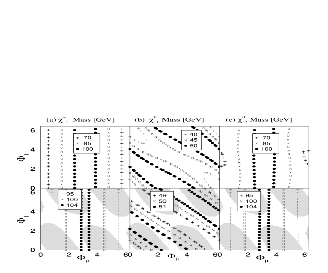
Figure 3 shows the mass spectrum of the lightest chargino $\tilde{\chi}^{\pm}_{1}$ and the neutralinos $\tilde{\chi}^{0}_{1,2}$ on the $\{\Phi_{\mu},\Phi_{1}\}$ plane for the scenarios ${\cal S}1$ and ${\cal S}2$. Each shaded area of the lower figures is excluded by the electron EDM constraints. Except for the region of $\Phi_{\mu}=0,\,2\pi$, the masses $m_{\tilde{\chi}^{\pm}_{1}}$ and $m_{\tilde{\chi}^{0}_{2}}$ are very similar in size and independent of $\Phi_{1}$ in both ${\cal S}1$ and ${\cal S}2$ while $m_{\tilde{\chi}^{0}_{1}}$ exhibits a strongly correlated dependence on the CP-violating phases. The masses $m_{\tilde{\chi}^{\pm}_{1}}$ and $m_{\tilde{\chi}^{0}_{2}}$ increase as $\Phi_{\mu}$ approaches $\pi$, while $m_{\tilde{\chi}^{0}_{1}}$ becomes maximal at certain non–trivial values of $\Phi_{\mu}$ and $\Phi_{1}$ in ${\cal S}1$. This implies that $m_{\tilde{\chi}^{0}_{1}}$ is strongly affected by a small value of $|\mu|$, while $m_{\tilde{\chi}^{\pm}_{1}}$ and $m_{\tilde{\chi}^{0}_{2}}$ are essentially determined by the SU(2)L gaugino mass $M_{2}$. The mass $m_{\tilde{\chi}^{0}_{1}}$ becomes smaller as the CP phases $\Phi_{1}$ and $\Phi_{\mu}$ approach the off–diagonal line on the plane, implying that the mass is a function of the sum $\Phi_{\mu}+\Phi_{1}$ of two CP phases to a very good approximation. Note that the masses $m_{\tilde{\chi}^{\pm}_{1}}$ and $m_{\tilde{\chi}^{0}_{1,2}}$ are more sensitive to the phases in ${\cal S}1$ because $|\mu|$ is comparable with $M_{2}$ and $m_{Z}$ in size in this scenario.

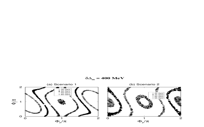
Although the chargino and neutralino masses cannot be separately measured at the Tevatron, the mass difference $\Delta_{m}\equiv m_{\tilde{\chi}^{0}_{2}}-m_{\tilde{\chi}^{0}_{1}}$ can be determined with a good precision [21] by measuring the end points of the invariant mass distribution of the same flavor but opposite sign dileptons from the neutralino decay. The precision of determining the mass difference is sensitive to the event rate and dependent on experimental capabilities. Deferring the discussion on these aspects to Sect. 4 we illustrate what information on the CP–violating phases the $\Delta_{m}$ measurement can provide us with. For that purpose, we assume the uncertainty for the mass difference to be 400 MeV and exhibit in Fig. 4 the allowed area of the CP–violating phases $\{\Phi_{\mu},\Phi_{1}\}$ for the SUSY parameters of (a) ${\cal S}1$ and (b) ${\cal S}2$. The figure clearly shows that the mass difference is a very sensitive probe of the CP–violating phases if the other real parameters are known; the sensitivity of the mass difference to the phases are enhanced when the gaugino and higgsino mass parameters are comparable to $m_{Z}$ in size.

4.2 Parton–level production helicity amplitudes

Although we are mainly interested in the production process $d\bar{u}\rightarrow\tilde{\chi}^{-}_{1}\tilde{\chi}^{0}_{2}$, we discuss in this section the associated production of any chargino and neutralino pair $d\bar{u}\rightarrow\tilde{\chi}^{-}_{i}\tilde{\chi}^{0}_{j}$ ($i=1,2$ and $j=1$ to $4$) for the sake of generality.

The parton–level production process $d\bar{u}\rightarrow\tilde{\chi}^{-}_{i}\tilde{\chi}^{0}_{j}$ is generated by the three mechanisms shown in Fig. 3: the $s$–channel $W^{-}$ exchange, the $t$–channel $\tilde{d}_{L}$ exchange and the $u$–channel $\tilde{u}_{L}$ exchange. Before presenting the explicit form for the production helicity amplitudes, we note that the chirality mixing of the first and second generation sfermions is proportional to the fermion mass much smaller than the beam energy of the Tevatron. Therefore, we can safely ignore the sfermion left–right chirality mixing in calculating the associated chargino-neutralino production rate so that the trilinear term $A_{f}$ does not play any role in the high energy process. The phase $\Phi_{3}$ of the gluino mass is irrelevant as well. Consequently, this associated production of chargino and neutralino and their subsequent decays involve only two CP–violating phases $\{\Phi_{\mu},\Phi_{1}\}$. With these good approximations and after an appropriate Fierz transformation to the $\tilde{u}_{L}$ and $\tilde{d}_{L}$–exchange amplitudes the transition matrix element can be written in the form

$\displaystyle T\left(d\bar{u}\rightarrow\tilde{\chi}^{-}_{i}\tilde{\chi}^{0}_{j}\right)=\frac{e^{2}}{s}Q^{ij}_{\alpha\beta}\left[\bar{v}(\bar{u})\gamma_{\mu}P_{\alpha}u(d)\right]\left[\bar{u}(\tilde{\chi}^{-}_{i})\gamma^{\mu}P_{\beta}v(\tilde{\chi}^{0}_{j})\right]\,.$ (48)

Here $Q_{\alpha\beta}$ are the so–called generalized bilinear charges [23], classified according to the chiralities $\alpha,\beta=L,R$ of the associated quark current and the chargino/neutralino current. The explicit forms of these bilinear charges are

$\displaystyle Q^{ij}_{LL}=\frac{D_{W}}{\sqrt{2}s_{W}^{2}}{\cal W}_{Lij}-\frac{D^{\tilde{d}_{L}}_{u}}{\sqrt{2}s_{W}}g_{Lij},$
$\displaystyle Q^{ij}_{LR}=\frac{D_{W}}{\sqrt{2}s_{W}^{2}}{\cal W}_{Rij}+\frac{D^{\tilde{u}_{L}}_{t}}{\sqrt{2}s_{W}}g_{Rij},$
$\displaystyle Q^{ij}_{RL}=0,\qquad Q^{ij}_{RR}=0.$ (49)

with the $s$–, $t$–, and $u$–channel propagators:

$\displaystyle D_{W}=\frac{s}{s-m^{2}_{W}+im_{W}\Gamma_{W}}\,,\qquad D^{\tilde{u}_{L}}_{t}=\frac{s}{t-m^{2}_{\tilde{u}_{L}}}\,,\qquad\ D^{\tilde{d}_{L}}_{u}=\frac{s}{u-m^{2}_{\tilde{d}_{L}}}\,,$ (50)

where $s=(p_{d}+p_{\bar{u}})^{2}$, $t=(p_{d}-p_{\tilde{\chi}^{-}_{i}})^{2}$ and $u=(p_{d}-p_{\tilde{\chi}^{0}_{j}})^{2}$, and the couplings ${\cal W}_{Lij}$, ${\cal W}_{Rij}$, $g_{Lij}$ and $g_{Rij}$ are given by

$\displaystyle{\cal W}_{Lij}=U_{Li1}N^{*}_{j2}+\frac{1}{\sqrt{2}}U_{Li2}N^{*}_{j3},$
$\displaystyle{\cal W}_{Rij}=U_{Ri1}N_{j2}-\frac{1}{\sqrt{2}}U_{Ri2}N_{j4},$
$\displaystyle g_{Lij}=\frac{U_{Li1}}{s_{W}c_{W}}\left[s_{W}(Q_{d}+\frac{1}{2})N^{*}_{j1}-\frac{1}{2}c_{W}N^{*}_{j2}\right],$
$\displaystyle g_{Rij}=\frac{U_{Ri1}}{s_{W}c_{W}}\left[s_{W}(Q_{u}-\frac{1}{2})N_{j1}+\frac{1}{2}c_{W}N_{j2}\right].$ (51)

Here $U_{Lij,Rij}$ ($N_{ij}$) are the chargino (neutralino) mixing matrix elements and $Q_{d}=-1/3$ and $Q_{u}=+2/3$ the electric charges for the down– and up–type quarks, respectively. Note that the coefficients $g_{Lij}$ and $g_{Rij}$ for the $t$– and $u$–channel diagrams are governed only by gaugino components of the chargino and neutralino while ${\cal W}_{Lij}$ and ${\cal W}_{Rij}$ are determined by both the gaugino and higgsino components.

Defining the $\tilde{\chi}^{-}_{i}$ flight direction with respect to the down quark momentum direction by $\Theta$, the explicit form of the production helicity amplitudes can be determined from eq. (48). In the limit of neglecting the initial $d$ and $u$ quark masses, the $d$ and $\bar{u}$ helicities are opposite to each other in all the exchange amplitudes, but the $\tilde{\chi}^{-}_{i}$ and $\tilde{\chi}^{0}_{j}$ helicities are less correlated due to the non–zero masses of the particles; the amplitudes with equal chargino/neutralino helicities $\propto m_{\tilde{\chi}^{-}_{i},\tilde{\chi}^{0}_{j}}/\sqrt{s}$ must vanish only for asymptotic energies. Denoting the down quark helicity by the first index, the $\tilde{\chi}^{-}_{i}$ and $\tilde{\chi}^{0}_{j}$ helicities by the remaining two indices, the production helicity amplitudes $T(\sigma;\lambda_{i},\lambda_{j})=2\pi\alpha\,\langle\sigma;\lambda_{i}\lambda_{j}\rangle$ can be derived by the so–called 2–component spinor technique [22], which yields

$\displaystyle\langle+;++\rangle=-\left[Q^{ij}_{RR}\sqrt{1-\eta^{2}_{+}}+Q^{ij}_{RL}\sqrt{1-\eta^{2}_{-}}\right]\sin\Theta\,,$
$\displaystyle\langle+;+-\rangle=-\left[Q^{ij}_{RR}\sqrt{(1+\eta_{+})(1+\eta_{-})}+Q^{ij}_{RL}\sqrt{(1-\eta_{+})(1-\eta_{-})}\right](1+\cos\Theta)\,,$
$\displaystyle\langle+;-+\rangle=+\left[Q^{ij}_{RR}\sqrt{(1-\eta_{+})(1-\eta_{-})}+Q^{ij}_{RL}\sqrt{(1+\eta_{+})(1+\eta_{-})}\right](1-\cos\Theta)\,,$
$\displaystyle\langle+;--\rangle=+\left[Q^{ij}_{RR}\sqrt{1-\eta^{2}_{-}}+Q^{ij}_{RL}\sqrt{1-\eta^{2}_{+}}\right]\sin\Theta\,,$
$\displaystyle\langle-;++\rangle=-\left[Q^{ij}_{LR}\sqrt{1-\eta^{2}_{+}}+Q^{ij}_{LL}\sqrt{1-\eta^{2}_{-}}\right]\sin\Theta\,,$
$\displaystyle\langle-;+-\rangle=+\left[Q^{ij}_{LR}\sqrt{(1+\eta_{+})(1+\eta_{-})}+Q^{ij}_{LL}\sqrt{(1-\eta_{+})(1-\eta_{-})}\right](1-\cos\Theta)\,,$
$\displaystyle\langle-;-+\rangle=-\left[Q^{ij}_{LR}\sqrt{(1-\eta_{+})(1-\eta_{-})}+Q^{ij}_{LL}\sqrt{(1+\eta_{+})(1+\eta_{-})}\right](1+\cos\Theta)\,,$
$\displaystyle\langle-;--\rangle=+\left[Q^{ij}_{LR}\sqrt{1-\eta^{2}_{-}}+Q^{ij}_{LL}\sqrt{1-\eta^{2}_{+}}\right]\sin\Theta\,,$ (52)

where $\eta_{\pm}=\lambda^{1/2}(1,\mu^{2}_{i},\mu^{2}_{j})\pm(\mu^{2}_{i}-\mu^{2}_{j})$ with $\mu^{2}_{i}\,(\mu^{2}_{j})=m^{2}_{\tilde{\chi}^{-}_{i}}(m^{2}_{\tilde{\chi}^{0}_{j}}/s)$ and $\lambda(x,y,z)=x^{2}+y^{2}+z^{2}-2xy-2yz-2zx$. If the arguments are not specified, then the notation $\lambda$ stands for $\lambda(1,\mu^{2}_{i},\mu^{2}_{j})$ in the following.

All physical observables constructed through the production process are determined by the production helicity amplitudes and expressed in a very simple form by sixteen quartic charges [23] containing the full information on the dynamical properties of the production process. These quartic charges are expressed in terms of the bilinear charges $Q^{ij}_{\alpha\beta}$ given by eq. (49) and classified according to their transformation properties under parity (P) as follows:
(a) Eight P–even terms:

$\displaystyle Q^{ij}_{1}=\frac{1}{4}\left[|Q^{ij}_{RR}|^{2}+|Q^{ij}_{LL}|^{2}+|Q^{ij}_{RL}|^{2}+|Q^{ij}_{LR}|^{2}\right]\,,$
$\displaystyle Q^{ij}_{2}=\frac{1}{2}\,\Re{\rm e}\!\left[Q^{ij}_{RR}Q^{ij*}_{RL}+Q^{ij}_{LL}Q^{ij*}_{LR}\right]\,,$
$\displaystyle Q^{ij}_{3}=\frac{1}{4}\left[|Q^{ij}_{LL}|^{2}+|Q^{ij}_{RR}|^{2}-|Q^{ij}_{RL}|^{2}-|Q^{ij}_{LR}|^{2}\right]\,,$
$\displaystyle Q^{ij}_{4}=\frac{1}{2}\,\Im{\rm m}\!\left[Q^{ij}_{RR}Q^{ij*}_{RL}+Q^{ij}_{LL}Q^{ij*}_{LR}\right]\,,$
$\displaystyle Q^{ij}_{5}=\frac{1}{2}\,\Re{\rm e}\!\left[Q^{ij}_{RR}Q^{ij*}_{LR}+Q^{ij}_{LL}Q^{ij*}_{RL}\right]\,,$
$\displaystyle Q^{ij}_{6}=\frac{1}{2}\,\Im{\rm m}\!\left[Q^{ij}_{RR}Q^{ij*}_{LR}+Q^{ij}_{LL}Q^{ij*}_{RL}\right]\,,$
$\displaystyle Q^{ij}_{7}=\Re{\rm e}\!\left[Q^{ij}_{RR}Q^{ij*}_{LL}\right]\,,$
$\displaystyle Q^{ij}_{8}=\Re{\rm e}\!\left[Q^{ij}_{RL}Q^{ij*}_{LR}\right]\,,$ (53)

(b) Eight P–odd terms:

$\displaystyle Q^{{}^{\prime}ij}_{1}=\frac{1}{4}\left[|Q^{ij}_{RR}|^{2}+|Q^{ij}_{RL}|^{2}-|Q^{ij}_{LR}|^{2}-|Q^{ij}_{LL}|^{2}\right]\,,$
$\displaystyle Q^{{}^{\prime}ij}_{2}=\frac{1}{2}\,\Re{\rm e}\!\left[Q^{ij}_{RR}Q^{ij*}_{RL}-Q^{ij}_{LL}Q^{ij*}_{LR}\right]\,,$
$\displaystyle Q^{{}^{\prime}ij}_{3}=\frac{1}{4}\left[|Q^{ij}_{RR}|^{2}+|Q^{ij}_{LR}|^{2}-|Q^{ij}_{RL}|^{2}-|Q^{ij}_{LL}|^{2}\right]\,,$
$\displaystyle Q^{{}^{\prime}ij}_{4}=\frac{1}{2}\,\Im{\rm m}\!\left[Q^{ij}_{RR}Q^{ij*}_{RL}-Q^{ij}_{LL}Q^{ij*}_{LR}\right]\,,$
$\displaystyle Q^{{}^{\prime}ij}_{5}=\frac{1}{2}\,\Re{\rm e}\!\left[Q^{ij}_{RR}Q^{ij*}_{LR}-Q^{ij}_{LL}Q^{ij*}_{RL}\right]\,,$
$\displaystyle Q^{{}^{\prime}ij}_{6}=\frac{1}{2}\,\Im{\rm m}\!\left[Q^{ij}_{RR}Q^{ij*}_{LR}-Q^{ij}_{LL}Q^{ij*}_{RL}\right]\,,$
$\displaystyle Q^{{}^{\prime}ij}_{7}=\Im{\rm m}\!\left[Q^{ij}_{RR}Q^{ij*}_{LL}\right]\,,$
$\displaystyle Q^{{}^{\prime}ij}_{8}=\Im{\rm m}\!\left[Q^{ij}_{RL}Q^{ij*}_{LR}\right]\,.$ (54)

We note that these 16 quartic charges comprise the most complete set for any fermion–pair production process in $d\bar{u}$ collisions when the quark masses are neglected. On the other hand, the quartic charges defined by an imaginary part of the bilinear–charge correlations might be non–vanishing only when there exist complex CP–violating couplings or/and CP–preserving phases like rescattering phases or finite widths of the intermediate particles. Therefore, such nonvanishing values of those quartic charges may signal CP violation in a given process.

4.3 Parton–level production cross section

The unpolarized differential production cross section of the parton–level process $d\bar{u}\rightarrow\tilde{\chi}^{-}_{i}\tilde{\chi}^{0}_{j}$ is obtained straightforwardly by taking the average/sum over the initial/final helicities:

$\displaystyle\frac{{\rm d}\hat{\sigma}}{{\rm d}\cos\Theta}(d\bar{u}\rightarrow\tilde{\chi}^{-}_{i}\tilde{\chi}^{0}_{j})=\frac{\pi\alpha^{2}}{32s}\lambda^{1/2}\,\sum_{\sigma\lambda_{i}\lambda_{j}}|\langle\sigma;\lambda_{i}\lambda_{j}\rangle|^{2}\,.$ (55)

Carrying out the sum, one finds the following expression for the parton level differential cross section in terms of the quartic charges:

$\displaystyle\frac{{\rm d}\hat{\sigma}}{{\rm d}\cos\Theta}(d\bar{u}\rightarrow\tilde{\chi}^{-}_{i}\tilde{\chi}^{0}_{j})$ $\displaystyle=$ $\displaystyle\frac{\pi\alpha^{2}}{8s}\lambda^{1/2}\bigg{\{}[4-(\eta_{+}-\eta_{-})^{2}+(\eta_{+}+\eta_{-})^{2}\cos^{2}\Theta]\,Q^{ij}_{1}\,,$ (56)
$\displaystyle+4\sqrt{(1-\eta^{2}_{+})(1-\eta^{2}_{-})}\,Q^{ij}_{2}+4(\eta_{+}+\eta_{-})\cos\Theta\,Q^{ij}_{3}\bigg{\}}\,.$

Thus, the three P–even quartic charges $Q^{ij}_{1}$, $Q^{ij}_{2}$ and $Q^{ij}_{3}$ determine the $\Theta$ dependence of the cross section completely.

The final cross section of the $\tilde{\chi}^{-}_{i}\tilde{\chi}^{0}_{j}$ production in $p\bar{p}$ collisions is obtained by convoluting the parton level cross section with a parton distribution and it is given by,

$\displaystyle\sigma(p\bar{p}\to\tilde{\chi}^{-}_{1}\tilde{\chi}^{0}_{2}+X)=\frac{\kappa}{3}\int_{0}^{1}\frac{dx}{x}\int_{\tau_{\rm min}}^{1}d\tau\left[f_{d/p}(x)f_{\bar{u}/\bar{p}}(\tau/x)+f_{\bar{u}/p}(x)f_{d/\bar{p}}(\tau/x)\right]\hat{\sigma}(\hat{s}=\tau s)\,,$ (57)

where $f$ are the respective parton fluxes in $p$ and $\bar{p}$ and $\tau_{\rm min}=(m_{\tilde{\chi}^{-}_{1}}+m_{\tilde{\chi}^{0}_{2}})^{2}/s$. We have used the CTEQ4m [24] parametrisation to obtain parton distribution setting the relevant QCD scale to the c.m. energy $\hat{s}$ of the parton level process. We take into account the dominant QCD radiative corrections to the production cross section by taking the parameter $\kappa=1.3$ [25] in eq. (57). The production cross section for the associated positively–charged chargino and neutralino pair is the same as its charge–conjugate one.

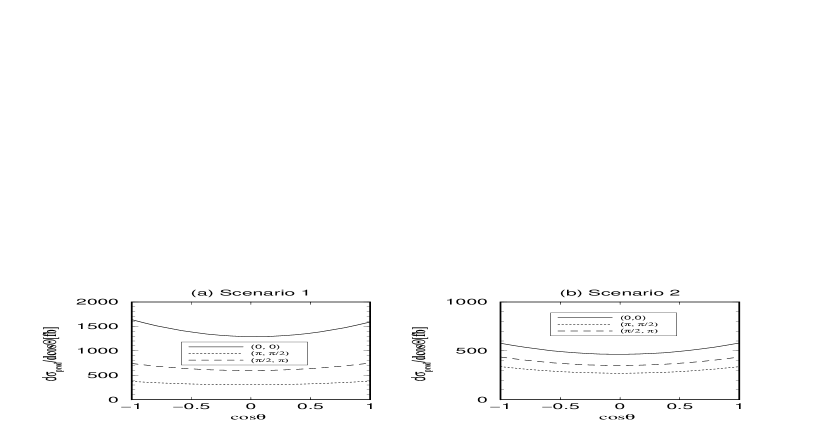
Figure 6 shows the distribution of the production cross section $\sigma(p\bar{p}\rightarrow\tilde{\chi}^{-}_{1}\tilde{\chi}^{0}_{2}+X)$ with the scattering angle $\Theta$ for various sets of $\{\Phi_{\mu},\Phi_{1}\}$ in the scenario ${\cal S}1$ and ${\cal S}2$ for a given c.m. energy of 1.8 TeV. We find that the production cross section is very sensitive to $\Phi_{\mu}$, but (almost) insensitive to $\Phi_{1}$. In order to look into this feature more clearly, we present in Fig. 7 the integrated production cross section $\sigma(p\bar{p}\rightarrow\tilde{\chi}^{-}_{1}\tilde{\chi}^{0}_{2}+X)$ on the $\{\Phi_{\mu},\Phi_{1}\}$ plane in (a) ${\cal S}1$ and (b) ${\cal S}2$, for which the constraints from the electron EDM are embedded on the plane. The results exhibit a few interesting aspects:

  • The differential cross section is (almost) forward-backward symmetric in both scenarios. This can be understood by noting the fact that the higgsino parts of ${\cal W}_{L,R}$ are suppressed in both scenarios due to large values of $|\mu|$ and that the relevant quartic charges $Q_{1,2}$ are forward–backward symmetric but $Q_{3}$ is proportional to $\cos\Theta$ to a good approximation due to the assumption $m_{\tilde{u}}=m_{\tilde{d}}$.

  • The large $|\mu|$ and small squark masses in the scenario ${\cal S}2$ reduce the production cross section due to a severe destructive interference between the $W$–exchange and squark–exchange diagrams. On the other hand, in the scenario ${\cal S}1$, the $t$– and $u$–channel contributions with the large squark masses can be ignored so that the lack of destructive interference yields a much larger value of the production cross section in the scenario.

  • Except for the region of $\Phi_{\mu}=0,2\pi$ in ${\cal S}1$, the integrated production cross section is almost independent of the phase $\Phi_{1}$ and it decreases as $\Phi_{\mu}$ approaches $\pi$ in both scenarios. This property is mainly set by the dependence of the chargino and neutralino masses on the CP–violating phases.

Consequently, the production cross section itself can be a very sensitive probe to the phase $\Phi_{\mu}$, but not to the phase $\Phi_{1}$.

4.4 Chargino and neutralino polarization vectors

The spin–1/2 chargino and neutralino through the parton–level process $d\bar{u}\rightarrow\tilde{\chi}^{-}_{i}\tilde{\chi}^{0}_{j}$ are in general polarized and their polarizations are reflected in the distributions of their decay products; $\tilde{\chi}^{-}_{i}\rightarrow\tilde{\chi}^{0}_{1}\,\ell^{-}\bar{\nu}_{\ell}$ and $\tilde{\chi}^{0}_{j}\rightarrow\tilde{\chi}^{0}_{1}\,\ell^{\prime+}\ell^{\prime-}$. In order to have a rough estimate of the effects of the CP–violating phases on the spin correlations, it is meaningful to investigate the chargino and neutralino polarizations in the parton–level production process $d\bar{u}\rightarrow\tilde{\chi}^{-}_{i}\tilde{\chi}^{0}_{j}$.

The polarization vector $\overrightarrow{\cal P}^{\tilde{\chi}^{-}_{i}}=({\cal P}^{\tilde{\chi}^{-}_{i}}_{L},{\cal P}^{\tilde{\chi}^{-}_{i}}_{T},{\cal P}^{\tilde{\chi}^{-}_{i}}_{N})$ of the produced chargino $\tilde{\chi}^{-}_{i}$ is defined in the rest frame in which the axis $\hat{z}\|L$ is in the flight direction of $\tilde{\chi}^{-}_{i}$, $\hat{x}\|T$ rotated counter–clockwise in the production plane, and $\hat{y}=\hat{z}\times\hat{x}\|N$ of the decaying chargino $\tilde{\chi}^{-}_{i}$. Accordingly, ${\cal P}^{\tilde{\chi}^{-}_{i}}_{L}$ denotes the component parallel to the $\tilde{\chi}^{-}_{i}$ flight direction in the c.m. frame, ${\cal P}^{\tilde{\chi}^{-}_{i}}_{T}$ the transverse component in the production plane, and ${\cal P}^{\tilde{\chi}^{-}_{i}}_{N}$ the component normal to the production plane. The three components of the chargino polarization vector can be expressed by the production helicity amplitudes (52) as

$\displaystyle{\cal P}^{\tilde{\chi}^{-}_{i}}_{L}=\frac{1}{4}\sum_{\sigma=\pm}\left\{|\langle\sigma;++\rangle|^{2}+|\langle\sigma;+-\rangle|^{2}-|\langle\sigma;-+\rangle|^{2}-|\langle\sigma;--\rangle|^{2}\right\}/{\cal N}\,,$
$\displaystyle{\cal P}^{\tilde{\chi}^{-}_{i}}_{T}=\frac{1}{2}\Re{\rm e}\bigg{\{}\sum_{\sigma=\pm}\left[\langle\sigma;++\rangle\langle\sigma;-+\rangle^{*}+\langle\sigma;--\rangle\langle\sigma;+-\rangle^{*}\right]\bigg{\}}/{\cal N}\,,$
$\displaystyle{\cal P}^{\tilde{\chi}^{-}_{i}}_{N}=\frac{1}{2}\Im{\rm m}\bigg{\{}\sum_{\sigma=\pm}\left[\langle\sigma;--\rangle\langle\sigma;+-\rangle^{*}-\langle\sigma;++\rangle\langle\sigma;-+\rangle^{*}\right]\bigg{\}}/{\cal N}\,,$ (58)

with the normalization corresponding to the unpolarized distribution

$\displaystyle{\cal N}=\frac{1}{4}\sum_{\lambda_{i}\lambda_{j}}\left[|\langle+;\lambda_{i}\lambda_{j}\rangle|^{2}+|\langle-;\lambda_{i}\lambda_{j}\rangle|^{2}\right]\,.$ (59)

The polarization vector of the neutralino $\tilde{\chi}^{0}_{j}$ can be obtained similarly from the production helicity amplitudes (52) by exchanging the chargino and neutralino helicities in eq. (58)

$\displaystyle{\cal P}^{\tilde{\chi}^{0}_{j}}_{L}=\frac{1}{4}\sum_{\sigma=\pm}\left\{|\langle\sigma;++\rangle|^{2}+|\langle\sigma;-+\rangle|^{2}-|\langle\sigma;+-\rangle|^{2}-|\langle\sigma;--\rangle|^{2}\right\}/{\cal N}\,,$
$\displaystyle{\cal P}^{\tilde{\chi}^{0}_{j}}_{T}=\frac{1}{2}\Re{\rm e}\bigg{\{}\sum_{\sigma=\pm}\left[\langle\sigma;++\rangle\langle\sigma;+-\rangle^{*}+\langle\sigma;--\rangle\langle\sigma;-+\rangle^{*}\right]\bigg{\}}/{\cal N}\,,$
$\displaystyle{\cal P}^{\tilde{\chi}^{0}_{j}}_{N}=\frac{1}{2}\Im{\rm m}\bigg{\{}\sum_{\sigma=\pm}\left[\langle\sigma;--\rangle\langle\sigma;-+\rangle^{*}-\langle\sigma;++\rangle\langle\sigma;+-\rangle^{*}\right]\bigg{\}}/{\cal N}\,.$ (60)

The longitudinal and transverse components of the polarization vectors are P–odd and CP–even, but the normal component is P–even and CP–odd so that the normal polarization component can be generated only by the complex production amplitudes. Certainly there exist non–trivial phases in CP non–invariant SUSY models. Also the non–zero width of the $Z$ boson and loop corrections generate non–trivial phases; however, the $Z$ boson width contribution to the normal polarization is negligible for high energies as mentioned before, and so are the radiative corrections. As a result the normal component is effectively generated by the genuine CP–odd phases of the couplings.

It is straightforward to find the normal polarization components of $\tilde{\chi}^{-}_{i}$ and $\tilde{\chi}^{0}_{j}$:

$\displaystyle{\cal P}^{\tilde{\chi}^{-}_{i}}_{N}=\frac{8}{\cal N}\,\lambda^{1/2}\mu_{i}\sin\Theta\,Q_{4}^{ij}\,,\qquad{\cal P}^{\tilde{\chi}^{0}_{j}}_{N}=\frac{8}{\cal N}\,\lambda^{1/2}\mu_{j}\sin\Theta\,Q_{4}^{ij}\,.$ (61)

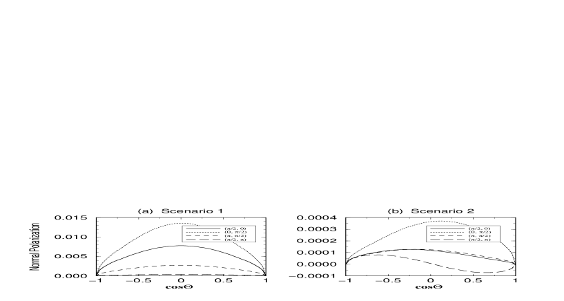
As expected from the CP properties of the normal components, they are determined by the CP–odd quartic charge $Q_{4}^{ij}$, which requires some complex couplings. In order to estimate the size of the normal polarization quantitatively, we present in Fig. 8 the normal polarization ${\cal P}^{\tilde{\chi}^{0}_{2}}_{N}$ for four different combinations of $\{\Phi_{\mu},\Phi_{1}\}$ in the scenarios ${\cal S}1$ and ${\cal S}2$ taking the parton–level c.m. energy of 300 GeV for the sake of illustration. [The chargino normal polarization is proportional to the neutralino normal polarization.] The expression (61) and Fig. 8 lead us to the following features:

  • The normal polarizations are suppressed near the thresholds or at high energies.

  • In the scenario ${\cal S}1$ with large squark masses, the quartic charge $Q_{4}^{ij}$ is forward-backward symmetric so that the normal polarizations also are forward–backward symmetric. However, this property is not maintained in the scenario ${\cal S}2$.

  • In both scenarios, the size of the normal polarizations is too small to measure the CP–violating phases directly in the production of the associated chargino and neutralino pair.

To conclude, it is likely that after applying the stringent EDM constraints to the CP–violating phases, we could not expect to have the normal polarizations of the chargino and neutralino large enough to be measured at the Tevatron.

5 Polarized Chargino and Neutralino Decays

The detection efficiency of the tri–lepton signatures at the Tevatron relies crucially on the branching fractions and distributions of the final three leptons, the latter of which depend on the polarizations of the decaying chargino and neutralino. To estimate the branching fractions, we need to calculate all the main partial decay widths that depend on the sparticle and Higgs–boson spectra in the MSSM. This section is devoted to a comprehensive discussion on the chargino and neutralino leptonic decays, including the polarizations of the decaying chargino and neutralino and the branching fractions. Firstly, we present the chargino and neutralino decay amplitudes in terms of the corresponding bilinear charges and the polarized decay distributions in terms of the quartic charges. Secondly, we calculate the decay density matrices by using the so–called Bouchiat–Michel formulas [26], that are to be used to form the complete production–decay spin/angular correlations. Finally, we estimate the branching fractions of the leptonic decays $\tilde{\chi}^{-}_{1}\rightarrow\tilde{\chi}^{0}_{1}\,\ell^{-}\bar{\nu}_{\ell}$ and $\tilde{\chi}^{0}_{2}\rightarrow\tilde{\chi}^{0}_{1}\,\ell^{\prime+}\ell^{\prime-}$ in the scenarios ${\cal S}1$ and ${\cal S}2$.

5.1 Polarized decay distributions

The diagrams contributing to the process $\tilde{\chi}^{-}_{i}\rightarrow\tilde{\chi}^{0}_{1}\,\ell^{-}\bar{\nu}_{\ell}$ and $\tilde{\chi}^{0}_{j}\rightarrow\tilde{\chi}^{0}_{1}\,\ell^{\prime-}\ell^{\prime+}$ with $\ell,\ell^{\prime}=e$, $\mu$ are shown in Figs. 9(a) and (b). Here, the exchange of the neutral and charged Higgs bosons [replacing the $W^{-}$ and $Z$ bosons] are neglected since the Yukawa couplings to the light first and second generation leptons are very small. In this case, all the components of the decay matrix elements are, after a simple Fierz transformation, written as

$\displaystyle{\cal D}\left(\tilde{\chi}^{-}_{i}\rightarrow\tilde{\chi}^{0}_{1}\,\ell^{-}\bar{\nu}_{\ell}\right)$ $\displaystyle=$ $\displaystyle\frac{e^{2}}{s^{\prime}}\,C^{i}_{\alpha\beta}\left[\bar{u}(\tilde{\chi}^{0}_{1})\gamma^{\mu}P_{\alpha}u(\tilde{\chi}^{-}_{i})\right]\left[\bar{u}(\ell^{-})\gamma_{\mu}P_{\beta}v(\bar{\nu}_{\ell})\right]\,,$
$\displaystyle{\cal D}\left(\tilde{\chi}^{0}_{j}\rightarrow\tilde{\chi}^{0}_{1}\,\ell^{\prime-}\ell^{\prime+}\right)$ $\displaystyle=$ $\displaystyle\frac{e^{2}}{s^{\prime\prime}}\,N^{j}_{\alpha\beta}\left[\bar{v}(\tilde{\chi}^{0}_{j})\gamma^{\mu}P_{\alpha}v(\tilde{\chi}^{0}_{1})\right]\left[\bar{u}(\ell^{\prime-})\gamma_{\mu}P_{\beta}v(\ell^{\prime+})\right]\,,$ (62)

where $\alpha,\beta=L,R$. Note that since the decaying neutralino is treated as an anti-particle in the associated production process $d\bar{u}\rightarrow\tilde{\chi}^{-}_{i}\tilde{\chi}^{0}_{j}$, the $v$ spinors for the decaying neutralino and the LSP appear in the expression for the neutralino leptonic decay. However, owing to the Majorana property of the neutralinos it does not matter whether the decay neutralino is treated as a particle or an anti-particle. The generalized bilinear charges $C^{i}_{\alpha\beta}$ for the chargino leptonic decay are given by

$\displaystyle C^{i}_{LL}=+\frac{D_{W}^{\prime}}{\sqrt{2}s_{W}^{2}}{\cal W}_{Li1}^{*}-\frac{D^{\tilde{l}_{L}}_{u^{\prime}}}{\sqrt{2}s_{W}}g^{*}_{Li1},$
$\displaystyle C^{i}_{RL}=-\frac{D_{W}^{\prime}}{\sqrt{2}s_{W}^{2}}{\cal W}_{i1R}^{*}+\frac{D^{\tilde{\nu}}_{t^{\prime}}}{\sqrt{2}s_{W}}g^{*}_{Ri1},$
$\displaystyle C^{i}_{LR}=C^{i}_{RR}=0,$ (63)

The couplings ${\cal W}_{Li1}$, ${\cal W}_{Ri1}$, $g_{Li1}$, and $g_{Ri1}$ are given in eq. (51). The $s^{\prime}$–, $t^{\prime}$– and $u^{\prime}$–channel propagators are

$\displaystyle D^{\prime}_{W}=\frac{s^{\prime}}{s^{\prime}-m^{2}_{W}+im_{W}\Gamma_{W}}\,,\qquad D^{\tilde{\nu}}_{t^{\prime}}=\frac{s^{\prime}}{t^{\prime}-m^{2}_{\tilde{\nu}}}\,,\qquad D^{\tilde{\l}_{L}}_{u^{\prime}}=\frac{s^{\prime}}{u^{\prime}-m^{2}_{\tilde{l}_{L}}}\,.$ (64)

where the Mandelstam variables $s^{\prime}$, $t^{\prime}$ and $u^{\prime}$ are defined in terms of the 4-momenta, $q_{0},\,q$ and $\bar{q}$, of $\tilde{\chi}^{0}_{1}$, $\ell^{-}$ and $\bar{\nu}_{\ell}$, respectively, as

$\displaystyle s^{\prime}=(q+\bar{q})^{2}\ \ ,\ \ t^{\prime}=(q_{0}+\bar{q})^{2}\ \ ,\ \ u^{\prime}=(q_{0}+q)^{2}\,,$ (65)

On the other hand, the generalized bilinear charges $N^{j}_{\alpha\beta}$ for the leptonic decay $\tilde{\chi}_{j}^{0}\rightarrow\tilde{\chi}^{0}_{1}\,\ell^{\prime+}\ell^{\prime-}$ are given by

$\displaystyle N^{j}_{LL}=+\frac{D_{Z}^{\prime\prime}}{s_{W}^{2}c_{W}^{2}}(s_{W}^{2}-\frac{1}{2}){\cal Z}_{j1}-D^{\tilde{\ell}^{\prime}_{L}}_{t^{\prime\prime}}\,h_{Lj1}\,,$
$\displaystyle N^{j}_{LR}=+\frac{D_{Z}^{\prime\prime}}{c_{W}^{2}}{\cal Z}_{j1}+D^{\tilde{\ell}^{\prime}_{R}}_{u^{\prime\prime}}\,h_{Rj1}\,,$
$\displaystyle N^{j}_{RL}=-\frac{D_{Z}^{\prime\prime}}{s_{W}^{2}c_{W}^{2}}(s_{W}^{2}-\frac{1}{2}){\cal Z}^{*}_{j1}+D^{\tilde{\ell}^{\prime}_{L}}_{u^{\prime\prime}}\,h^{*}_{Lj1}\,,$
$\displaystyle N^{j}_{RR}=-\frac{D_{Z}^{\prime\prime}}{c_{W}^{2}}{\cal Z}^{*}_{j1}-D^{\tilde{\ell}^{\prime}_{R}}_{t^{\prime\prime}}\,h^{*}_{Rj1}\,,$ (66)

where the $s^{\prime\prime}$–, $t^{\prime\prime}$– and $u^{\prime\prime}$–channel propagators are

$\displaystyle D_{Z}^{\prime\prime}=\frac{s^{\prime\prime}}{s^{\prime\prime}-m^{2}_{Z}+im_{Z}\Gamma_{Z}},\qquad D^{\tilde{\l}_{L,R}}_{t^{\prime\prime}}=\frac{s^{\prime\prime}}{t^{\prime\prime}-m^{2}_{\tilde{l}_{L,R}}},\qquad D^{\tilde{\l}_{L,R}}_{u^{\prime\prime}}=\frac{s^{\prime\prime}}{u^{\prime\prime}-m^{2}_{\tilde{l}_{L,R}}},$ (67)

with the Mandelstam variables $s^{\prime\prime}=(q^{\prime}+\bar{q}^{\prime})^{2}$, $t^{\prime\prime}=(q_{0}^{\prime}+\bar{q}^{\prime})^{2}$ and $u^{\prime\prime}=(q_{0}^{\prime}+q^{\prime})^{2}$ in terms of the 4–momenta, $q^{\prime}_{0},\,q^{\prime}$ and $\bar{q}^{\prime}$, of $\tilde{\chi}^{0}_{1}$, $\ell^{\prime-}$ and $\ell^{\prime+}$, respectively. The couplings ${\cal Z}_{ij}$, $h_{Lij}$ and $h_{Rij}$ are expressed in terms of neutralino diagonalization matrix elements $N_{ij}$ as

$\displaystyle{\cal Z}_{ij}=\frac{1}{2}\left[N_{i3}N^{*}_{j3}-N_{i4}N^{*}_{j4}\right]\,,$
$\displaystyle h_{Lij}=\frac{1}{4s_{W}^{2}c_{W}^{2}}(N_{i2}c_{W}+N_{i1}s_{W})(N^{*}_{j2}c_{W}+N^{*}_{j1}s_{W})\,,$
$\displaystyle h_{Rij}=\frac{1}{c_{W}^{2}}N_{i1}N^{*}_{j1}\,,$ (68)

and they satisfy the Hermiticity relations reflecting the CP relations

$\displaystyle{\cal Z}_{ij}={\cal Z}^{*}_{ji}\,,\qquad h_{Lij}=h^{*}_{Lji}\,,\qquad h_{Rij}=h^{*}_{Rji}\,.$ (69)

Note that ${\cal Z}_{j1}$ is governed by the higgsino components of $\tilde{\chi}^{0}_{j}$ while $h_{Lj1}$ and $h_{Rj1}$ are determined by the gaugino components of the neutralino. Therefore, as will be shown later, ${\cal Z}_{21}$ are suppressed in the scenario ${\cal S}2$ with a large $|\mu|$, while the $t$– and $u$–channel diagrams are suppressed in the scenario ${\cal S}1$ with large selectron masses.

Applying the polarization projection operator of the chargino to the amplitude squared of the chargino leptonic decay $\tilde{\chi}^{-}_{i}\rightarrow\tilde{\chi}^{0}_{1}\,\ell^{-}\bar{\nu}_{\ell}$ yields the polarized decay distributions with the polarization vector $n_{i}^{\mu}$ of the chargino $\tilde{\chi}^{-}_{i}$:

$\displaystyle|{\cal D}|^{2}(n_{i})$ $\displaystyle=$ $\displaystyle-4(t^{\prime}-m_{\chi_{i}^{-}}^{2})(t^{\prime}-m_{\chi_{1}^{0}}^{2})(C^{i}_{1}-C^{i}_{3})-4(u^{\prime}-m_{\chi_{i}^{-}}^{2})(u^{\prime}-m_{\chi_{1}^{0}}^{2})(C^{i}_{1}+C^{i}_{3})$ (70)
$\displaystyle-8m_{\tilde{\chi}^{-}_{i}}m_{\tilde{\chi}^{0}_{1}}s^{\prime}C^{i}_{2}$
$\displaystyle-8(n_{i}\cdot\bar{q})\left[m_{\tilde{\chi}^{-}_{i}}(m_{\tilde{\chi}^{0}_{1}}^{2}-u^{\prime})(C^{i\prime}_{1}+C^{i\prime}_{3})+m_{\tilde{\chi}^{0}_{1}}(m_{\tilde{\chi}^{-}_{i}}^{2}-t^{\prime})C^{i\prime}_{2}\right]$
$\displaystyle+8(n_{i}\cdot q)\left[-m_{\tilde{\chi}^{-}_{i}}(m_{\tilde{\chi}^{0}_{1}}^{2}-t^{\prime})(C^{i\prime}_{1}-C^{i\prime}_{3})+m_{\tilde{\chi}^{0}_{1}}(m_{\tilde{\chi}^{-}_{i}}^{2}-u^{\prime})C^{i\prime}_{2}\right]$
$\displaystyle-16\,m_{\tilde{\chi}^{0}_{1}}\langle q_{i}n_{i}q\bar{q}\rangle C^{i}_{4}\,,$

where $\langle q_{i}n_{i}q_{1}\bar{q}_{2}\rangle\equiv\epsilon_{\mu\nu\rho\sigma}q_{i}^{\mu}n_{i}^{\nu}q^{\rho}\bar{q}^{\sigma}$ with the convention $\epsilon_{0123}=+1$. Here, the quartic charges $\{C_{i1}$ - $C_{i4}\}$ and $\{C^{\prime}_{i1}$ - $C^{\prime}_{i3}\}$ for the chargino decays are defined by

$\displaystyle C^{i}_{1}=\frac{1}{4}\left[|C^{i}_{RR}|^{2}+|C^{i}_{LL}|^{2}+|C^{i}_{RL}|^{2}+|C^{i}_{LR}|^{2}\right]\,,$
$\displaystyle C^{i}_{2}=\frac{1}{2}\Re{\rm e}\left[C^{i}_{RR}C^{i*}_{LR}+C^{i}_{LL}C^{i*}_{RL}\right]\,,$
$\displaystyle C^{i}_{3}=\frac{1}{4}\left[|C^{i}_{LL}|^{2}+|C^{i}_{RR}|^{2}-|C^{i}_{RL}|^{2}-|C^{i}_{LR}|^{2}\right]\,,$
$\displaystyle C^{i}_{4}=\frac{1}{2}\Im{\rm m}\left[C^{i}_{RR}C^{i*}_{LR}+C^{i}_{LL}C^{i*}_{RL}\right]\,,$
$\displaystyle C^{i\prime}_{1}=\frac{1}{4}\left[|C^{i}_{RR}|^{2}+|C^{i}_{RL}|^{2}-|C^{i}_{LR}|^{2}-|C^{i}_{LL}|^{2}\right]\,,$
$\displaystyle C^{i\prime}_{2}=\frac{1}{2}\Re{\rm e}\left[C^{i}_{RR}C^{i*}_{LR}-C^{i}_{LL}C^{i*}_{RL}\right]\,,$
$\displaystyle C^{i\prime}_{3}=\frac{1}{4}\left[|C^{i}_{RR}|^{2}+|C^{i}_{LR}|^{2}-|C^{i}_{RL}|^{2}-|C^{i}_{LL}|^{2}\right]\,.$ (71)

The polarized distribution with a polarization vector $\bar{n}_{j}^{\mu}$ of the neutralino decay $\tilde{\chi}^{0}_{i}\rightarrow\tilde{\chi}^{0}_{1}\,\ell^{\prime-}\ell^{\prime+}$ can be derived in a straightforward way

$\displaystyle|\bar{\cal D}|^{2}(\bar{n}_{j})$ $\displaystyle=$ $\displaystyle-4(t^{\prime\prime}-m_{\tilde{\chi}^{0}_{j}}^{2})(t^{\prime\prime}-m_{\tilde{\chi}^{0}_{1}}^{2})(N^{j}_{1}+N^{j}_{3})-4(u^{\prime\prime}-m_{\tilde{\chi}^{0}_{j}}^{2})(u^{\prime\prime}-m_{\tilde{\chi}^{0}_{1}}^{2})(N^{j}_{1}-N^{j}_{3})$ (72)
$\displaystyle-8m_{\tilde{\chi}^{0}_{j}}m_{\tilde{\chi}^{0}_{1}}s^{\prime\prime}N^{j}_{2}$
$\displaystyle-8(\bar{n}_{j}\cdot\bar{q}^{\prime})\left[-m_{\tilde{\chi}^{0}_{j}}(m_{\tilde{\chi}^{0}_{1}}^{2}-u^{\prime\prime})(N^{j\prime}_{1}-N^{j\prime}_{3})+m_{\tilde{\chi}^{0}_{1}}(m_{\tilde{\chi}^{0}_{j}}^{2}-t^{\prime\prime})N^{j\prime}_{2}\right]$
$\displaystyle+8(\bar{n}_{j}\cdot q^{\prime})\left[m_{\tilde{\chi}^{0}_{j}}(m_{\tilde{\chi}^{0}_{1}}^{2}-t^{\prime\prime})(N^{j\prime}_{1}+N^{j\prime}_{3})+m_{\tilde{\chi}^{0}_{1}}(m_{\tilde{\chi}^{0}_{j}}^{2}-u^{\prime\prime})N^{j\prime}_{2}\right]$
$\displaystyle+16\,m_{\tilde{\chi}^{0}_{1}}\langle q_{j}\bar{n}_{j}q^{\prime}\bar{q}^{\prime}\rangle N^{j}_{4}\,,$

The quartic charges for the neutralino decay case can be obtained from the bilinear charges $N^{j}_{\alpha\beta}$ in the same way as the chargino quartic charges are defined in terms of the bilinear charges $C^{i}_{\alpha\beta}$. Related to CP violation it is worthwhile to note that the quartic charges $C^{i}_{4}$ and $N^{j}_{4}$ manifest CP violation in the theory.

For the sake of subsequent discussion of the spin/angular correlations between the production and decay processes, we construct the decay density matrix $\rho_{\lambda\lambda^{\prime}}\sim{\cal D}_{\lambda}{\cal D}^{*}_{\lambda^{\prime}}$. In general, the decay amplitude for a spin–1/2 particle and its complex conjugate can be expressed as

$\displaystyle{\cal D}(\lambda)=\Gamma\,u(q,\lambda),\qquad{\cal D}^{*}(\lambda^{\prime})=\bar{u}(q,\lambda^{\prime})\,\bar{\Gamma},$ (73)

with the general spinor structure $\Gamma$ and $\bar{\Gamma}=\gamma^{0}\Gamma^{\dagger}$. Then we use the general formalism to calculate the decay density matrix involving a particle with 4–momentum $q$ and mass $m$ by introducing three spacelike 4–vectors $n^{a}_{\mu}$ ($a=1,2,3$) which together with $q/m\equiv n^{0}$ form an orthonormal set:

$\displaystyle g^{\mu\nu}\,n^{a}_{\mu}n^{b}_{\nu}=g^{ab},\qquad g_{ab}\,n^{a}_{\mu}n^{b}_{\nu}=g_{\mu\nu}\,,$ (74)

with $g^{\mu\nu},\,g^{ab}={\rm diag}\,(1,-1,-1,-1)$ $(a,b=0,1,2,3)$. A convenient choice for the explicit form of ${n^{a}}^{\mu}$ is in a coordinate system where the direction of the three–momentum of the particle is $\hat{q}=(\sin\theta,0,\cos\theta)$ lying on the $x$-$z$ plane:

$\displaystyle{n^{1}}^{\mu}=(0,\cos\theta,0,-\sin\theta)\,,\qquad{n^{2}}^{\mu}=(0,0,1,0)\,,\qquad{n^{3}}^{\mu}=\frac{1}{m}\left(|\vec{q}|,E\hat{q}\right)\,.$ (75)

Then in the given reference frame, the three 4–vectors as defined in the above equation describe the transverse, normal and longitudinal polarization of the decaying particle, respectively.

With the four–dimensional orthonormal basis of the 4–vectors $\{n^{0},n^{1},n^{2},n^{3}\}$, we can derive the so–called Bouchiat–Michel formulas [26] for $u$ and $v$ spinors

$\displaystyle u(q,\lambda)\bar{u}(q,\lambda^{\prime})=\frac{1}{2}\left[\delta_{\lambda\lambda^{\prime}}+\gamma_{5}\not\!{n}^{a}\tau^{a}_{\lambda^{\prime}\lambda}\right](\not\!{q}+m)\,,$
$\displaystyle v(q,\lambda)\bar{v}(q,\lambda^{\prime})=\frac{1}{2}\left[\delta_{\lambda\lambda^{\prime}}+\gamma_{5}\not\!{n}^{a}\tau^{a}_{\lambda\lambda^{\prime}}\right](\not\!{q}-m)\,,$ (76)

with $\lambda,\lambda^{\prime}=\pm$. These formulas enable us to compute the squared, normalized decay density matrix $\rho_{\lambda\lambda^{\prime}}$ as follows:

$\displaystyle\rho_{\lambda\lambda^{\prime}}\equiv\frac{{\cal D}(\lambda){\cal D}^{*}(\lambda^{\prime})}{\sum_{\lambda}|{\cal D}(\lambda)|^{2}}=\frac{1}{2}\left[\delta_{\lambda\lambda^{\prime}}+\frac{Y^{a}}{X}\tau^{a}_{\lambda^{\prime}\lambda}\right]$ (77)

where $\tau^{a}$ ($a=1,2,3$) are the Pauli matrices. The three functions $X$ and $Y^{a}$ ($a=1,2,3$) for the chargino leptonic decay $\tilde{\chi}^{-}_{i}\rightarrow\tilde{\chi}^{0}_{1}\,\ell^{-}\bar{\nu}_{\ell}$ and the three functions $\bar{X}$ and $\bar{Y}^{a}$ ($a=1,2,3$) for the neutralino leptonic decay $\tilde{\chi}^{0}_{j}\rightarrow\tilde{\chi}^{0}_{1}\,\ell^{\prime+}\ell^{\prime-}$ can be obtained easily as

$\displaystyle X$ $\displaystyle=$ $\displaystyle-8(t^{\prime}-m_{\chi_{i}^{-}}^{2})(t^{\prime}-m_{\chi_{1}^{0}}^{2})(C^{i}_{1}-C^{i}_{3})-8(u^{\prime}-m_{\chi_{i}^{-}}^{2})(u^{\prime}-m_{\chi_{1}^{0}}^{2})(C^{i}_{1}+C^{i}_{3})$
$\displaystyle-16\,m_{\tilde{\chi}^{-}_{i}}m_{\tilde{\chi}^{0}_{1}}s^{\prime}C^{i}_{2},$
$\displaystyle Y^{a}$ $\displaystyle=$ $\displaystyle-16(n_{i}^{a}\cdot\bar{q})\left[m_{\tilde{\chi}^{-}_{i}}(m_{\tilde{\chi}^{0}_{1}}^{2}-u^{\prime})(C^{i\prime}_{1}+C^{i\prime}_{3})+m_{\tilde{\chi}^{0}_{1}}(m_{\tilde{\chi}^{-}_{i}}^{2}-t^{\prime})C^{i\prime}_{2}\right]$ (78)
$\displaystyle+16(n_{i}^{a}\cdot q)\left[-m_{\tilde{\chi}^{-}_{i}}(m_{\tilde{\chi}^{0}_{1}}^{2}-t^{\prime})(C^{i\prime}_{1}-C^{i\prime}_{3})+m_{\tilde{\chi}^{0}_{1}}(m_{\tilde{\chi}^{-}_{i}}^{2}-u^{\prime})C^{i\prime}_{2}\right]$
$\displaystyle-32\,m_{\tilde{\chi}^{0}_{1}}\langle q_{i}n_{i}^{a}q\bar{q}\rangle C^{i}_{4}\,,$

and

$\displaystyle\bar{X}$ $\displaystyle=$ $\displaystyle-8(t^{\prime\prime}-m_{\tilde{\chi}^{0}_{j}}^{2})(t^{\prime\prime}-m_{\tilde{\chi}^{0}_{1}}^{2})(N^{j}_{1}+N^{j}_{3})-8(u^{\prime\prime}-m_{\tilde{\chi}^{0}_{j}}^{2})(u^{\prime\prime}-m_{\tilde{\chi}^{0}_{1}}^{2})(N^{j}_{1}-N^{j}_{3})$
$\displaystyle-16\,m_{\tilde{\chi}^{0}_{j}}m_{\tilde{\chi}^{0}_{1}}s^{\prime\prime}N^{j}_{2},$
$\displaystyle\bar{Y}^{a}$ $\displaystyle=$ $\displaystyle-16(\bar{n}_{j}^{a}\cdot\bar{q}^{\prime})\left[-m_{\tilde{\chi}^{0}_{j}}(m_{\tilde{\chi}^{0}_{1}}^{2}-u^{\prime\prime})(N^{j\prime}_{1}-N^{j\prime}_{3})+m_{\tilde{\chi}^{0}_{1}}(m_{\tilde{\chi}^{0}_{j}}^{2}-t^{\prime\prime})N^{j\prime}_{2}\right]$ (79)
$\displaystyle+16(\bar{n}_{j}^{a}\cdot q^{\prime})\left[+m_{\tilde{\chi}^{0}_{j}}(m_{\tilde{\chi}^{0}_{1}}^{2}-t^{\prime\prime})(N^{j\prime}_{1}+N^{j\prime}_{3})+m_{\tilde{\chi}^{0}_{1}}(m_{\tilde{\chi}^{0}_{j}}^{2}-u^{\prime\prime})N^{j\prime}_{2}\right]$
$\displaystyle+32\,m_{\tilde{\chi}^{0}_{1}}\langle q_{j}\bar{n}_{j}^{a}q^{\prime}\bar{q}^{\prime}\rangle N^{j}_{4}\,,$

where $n_{i}^{a}$ and $\bar{n}_{j}^{a}$ is the polarization vector of the decaying chargino and neutralino, respectively.

5.2 Branching fractions

The main decay modes of the lightest chargino $\tilde{\chi}^{-}_{1}$ and the next–lightest neutralino $\tilde{\chi}^{0}_{2}$ can be classified as follows:

$\displaystyle\tilde{\chi}^{-}_{1}$ $\displaystyle\rightarrow$ $\displaystyle W^{*}\tilde{\chi}^{0}_{1},\,H^{*}\tilde{\chi}^{0}_{1}\rightarrow\tilde{\chi}^{0}_{1}\,\ell^{-}\bar{\nu}_{\ell},\,\tilde{\chi}^{0}_{1}q\bar{q^{\prime}}\,,$
$\displaystyle\tilde{\chi}^{-}_{1}$ $\displaystyle\rightarrow$ $\displaystyle\ell\tilde{\nu}^{*},\,\nu\tilde{\ell}^{*},\,q\tilde{q^{\prime}}^{*}\rightarrow\tilde{\chi}^{0}_{1}\,\ell^{-}\bar{\nu}_{\ell},\,\tilde{\chi}^{0}_{1}q\bar{q^{\prime}}\,,$
$\displaystyle\tilde{\chi}^{0}_{2}$ $\displaystyle\rightarrow$ $\displaystyle Z^{*}\tilde{\chi}^{0}_{1},\,H^{*}\tilde{\chi}^{0}_{1}\rightarrow\tilde{\chi}^{0}_{1}\,\ell^{+}\ell^{-},\,\tilde{\chi}^{0}_{1}q\bar{q}\,,$
$\displaystyle\tilde{\chi}^{0}_{2}$ $\displaystyle\rightarrow$ $\displaystyle\ell\tilde{\ell}^{*},\nu\tilde{\nu}^{*},\,q\tilde{q}^{*}\rightarrow\tilde{\chi}^{0}_{1}\,\ell^{+}\ell^{-},\,\tilde{\chi}^{0}_{1}q\bar{q}\,,$ (80)

with $q$ and $q^{\prime}$ belonging to the same SU(2)L multiplet. Besides, if the mass $m_{\tilde{\chi}^{\pm}_{1}}$ is smaller than the neutralino mass $m_{\tilde{\chi}^{0}_{2}}$, the lightest chargino $\tilde{\chi}^{\pm}_{1}$ can take part in the neutralino decay via the processes $\tilde{\chi}^{0}_{2}\rightarrow\tilde{\chi}^{\pm}_{1}W^{\mp*},\,\tilde{\chi}^{\pm}_{1}H^{\mp*}$ and vice versa. Concerning the main decay modes, there are several aspects to be noted:

  • For the first and second generation leptons, the Higgs–exchange diagrams are suppressed if $\tan\beta$ is not very large and there is no generational mixing in the slepton sector.

  • The experimental bounds on the Higgs particles are very stringent so that the two–body decays $\tilde{\chi}^{0}_{2}\rightarrow H\tilde{\chi}^{0}_{1}$, $\tilde{\chi}^{0}_{2}\rightarrow H^{\pm}\tilde{\chi}^{\mp}_{1}$, and $\tilde{\chi}^{-}_{1}\rightarrow H^{-}\tilde{\chi}^{0}_{1}$ are expected to be not available or at least strongly suppressed. If these decay modes open up, it could then spoil the tri–lepton signal.

  • The lightest chargino and the second–lightest neutralino are almost degenerate in the gaugino–dominated parameter space so that the charged decays such as $\tilde{\chi}^{0}_{2}\rightarrow\tilde{\chi}^{\pm}_{1}\,\ell^{\mp}\nu_{\ell}$ and $\tilde{\chi}^{-}_{1}\rightarrow\tilde{\chi}^{0}_{2}\,\ell^{-}\bar{\nu}_{\ell}$ will be highly suppressed.

Keeping in mind the above subtle aspects, we calculate the branching fractions ${\cal B}(\tilde{\chi}^{-}_{1}\rightarrow\tilde{\chi}^{0}_{1}\,\ell^{-}\bar{\nu}_{\ell})$ and ${\cal B}(\tilde{\chi}^{0}_{2}\rightarrow\tilde{\chi}^{0}_{1}\,\ell^{\prime+}\ell^{\prime-})$ fully incorporating all the possible decay modes of the neutralino $\tilde{\chi}^{0}_{2}$ but neglecting the Higgs-exchange contributions in both scenarios.

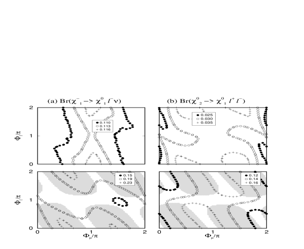
We present in Fig. 10 the branching fractions ${\cal B}(\tilde{\chi}^{-}_{1}\rightarrow\tilde{\chi}^{0}_{1}\,\ell^{-}\bar{\nu}_{\ell})$ and ${\cal B}(\tilde{\chi}^{0}_{2}\rightarrow\tilde{\chi}^{0}_{1}\,\ell^{\prime+}\ell^{\prime-})$ for $\ell\,\ell^{\prime}=e$ or $\mu$ in ${\cal S}1$ (two upper figures) and in ${\cal S}2$ (two lower figures). In the scenario ${\cal S}1$ the branching fraction ${\cal B}(\tilde{\chi}^{-}_{1}\rightarrow\tilde{\chi}^{0}_{1}\,\ell^{-}\bar{\nu}_{\ell})$ is almost constant over the whole space of the phases and the branching fraction ${\cal B}(\tilde{\chi}^{0}_{2}\rightarrow\tilde{\chi}^{0}_{1}\,\ell^{\prime+}\ell^{\prime-})$ is very small and sensitive to the phases only around $\Phi_{1}$ around $\Phi_{\mu}=0,2\pi$. The insensitivity of both branching fractions to the phases in ${\cal S}1$ is due to the fact that the $t$– and $u$–channel contributions are suppressed due to large slepton masses and the couplings ${\cal W}_{L11},{\cal W}_{R11}$, and ${\cal Z}_{21}$ for the $s$–channel contributions are not so much sensitive to $\Phi_{\mu}$ and $\Phi_{1}$. On the contrary, the branching fractions are rather sensitive to $\Phi_{\mu}$ and $\Phi_{1}$ in the scenario ${\cal S}2$. It is interesting that the branching fraction ${\cal B}(\tilde{\chi}^{-}_{1}\rightarrow\tilde{\chi}^{0}_{1}\,\ell^{-}\bar{\nu}_{\ell})$ can be minimal for certain non–trivial values of the CP–violating phases. We note that the branching fraction ${\cal B}(\tilde{\chi}^{0}_{2}\rightarrow\tilde{\chi}^{0}_{1}\,\ell^{\prime+}\ell^{\prime-})$ is greatly enhanced in the scenario ${\cal S}2$; this stems from the fact that the slepton–exchange contributions due to mainly the gaugino components of the neutralinos become dominant for the small slepton masses and the large value of $|\mu|$. On the contrary, the branching fraction ${\cal B}(\tilde{\chi}^{-}_{1}\rightarrow\tilde{\chi}^{0}_{1}\,\ell^{-}\bar{\nu}_{\ell})$ is not so different in size between the two scenarios, but the branching fraction becomes more sensitive to the CP–violating phases in the scenario ${\cal S}2$.

In summary, the branching fractions ${\cal B}(\tilde{\chi}^{-}_{1}\rightarrow\tilde{\chi}^{0}_{1}\,\ell^{-}\bar{\nu}_{\ell})$ and ${\cal B}(\tilde{\chi}^{0}_{2}\rightarrow\tilde{\chi}^{0}_{1}\,\ell^{\prime+}\ell^{\prime-})$ are not so strongly dependent on the CP–violating phases $\{\Phi_{\mu},\Phi_{1}\}$, but the branching fraction ${\cal B}(\tilde{\chi}^{0}_{2}\rightarrow\tilde{\chi}^{0}_{1}\,\ell^{\prime+}\ell^{\prime-})$ is very sensitive to the slepton masses.

6 Spin/Angular Correlated Observables

6.1 Correlations between production and decay

In this section we provide a general formalism to describe the spin/angular correlations between the production process $d\bar{u}\rightarrow\tilde{\chi}^{-}_{i}\tilde{\chi}^{0}_{j}$ and the sequential leptonic decays of $\tilde{\chi}^{-}_{i}$ and $\tilde{\chi}^{0}_{j}$. Formally we can have the spin/angular correlated distribution by taking the sum over the helicity indices of the intermediate chargino and neutralino states and folding with the chargino–neutralino leptonic decay density matrix $\rho_{\lambda\lambda^{\prime}}$ and $\bar{\rho}_{\bar{\lambda}\bar{\lambda^{\prime}}}$ with the matrix squared for the production helicity amplitudes:

$\displaystyle\sum_{\rm corr}$ $\displaystyle\equiv$ $\displaystyle\pi^{2}\alpha^{2}\sum_{\lambda\lambda^{\prime}}\sum_{\bar{\lambda}\bar{\lambda^{\prime}}}\sum_{\sigma}\langle\sigma;\lambda\bar{\lambda}\rangle\langle\sigma;\lambda^{\prime}\bar{\lambda^{\prime}}\rangle^{*}\rho_{\lambda\lambda^{\prime}}\bar{\rho}_{\bar{\lambda}\bar{\lambda^{\prime}}}$ (81)
$\displaystyle=$ $\displaystyle\pi^{2}\alpha^{2}\bigg{[}\Sigma_{\rm unp}+P_{z}{\cal P}+\bar{P}_{z}\bar{{\cal P}}+P_{x}{\cal U}+P_{y}\bar{{\cal U}}+\bar{P}_{x}{\cal V}+\bar{P}_{y}\bar{{\cal V}}+P_{z}\bar{P}_{z}{\cal Q}$
$\displaystyle\hskip 11.38092pt+P_{x}\bar{P}_{z}{\cal W}+P_{y}\bar{P}_{z}\bar{{\cal W}}+\bar{P}_{x}P_{z}{\cal X}+\bar{P}_{y}P_{z}\bar{{\cal X}}+(P_{x}\bar{P}_{x}-P_{y}\bar{P}_{y}){\cal Y}$
$\displaystyle\hskip 11.38092pt+(P_{x}\bar{P}_{y}+P_{y}\bar{P}_{x})\,\bar{{\cal Y}}+(P_{x}\bar{P}_{x}+P_{y}\bar{P}_{y})\,{\cal Z}+(P_{y}\bar{P}_{x}-P_{x}\bar{P}_{y})\,\bar{{\cal Z}}\bigg{]},$

where the functions $P_{x,y,z}$ and $\bar{P}_{x,y,z}$ depending on the chargino and neutralino decay distributions, respectively,

$\displaystyle P_{x}=\frac{Y^{1}}{X}\,,\qquad P_{y}=\frac{Y^{2}}{X}\,,\qquad P_{z}=\frac{Y^{3}}{X}\,,$
$\displaystyle\bar{P}_{x}=\frac{\bar{Y}^{1}}{\bar{X}}\,,\qquad\bar{P}_{y}=\frac{\bar{Y}^{2}}{\bar{X}}\,,\qquad\bar{P}_{z}=\frac{\bar{Y}^{3}}{\bar{X}}\,,$ (82)

serve as the polarimeters to extract the spin–spin correlations of the chargino $\tilde{\chi}^{-}_{i}$ and the neutralino $\tilde{\chi}^{0}_{j}$ in the production process. The sixteen coefficients are combinations of the production helicity amplitudes, corresponding to the unpolarized cross section, $2\times 3$ polarization components and $3\times 3$ spin–spin correlations.


(i) Unpolarized part:

$\displaystyle\Sigma_{\rm unpol}$ $\displaystyle=$ $\displaystyle\frac{1}{4}\sum_{\sigma=\pm}\bigg{[}|\langle\sigma;++\rangle|^{2}+|\langle\sigma;+-\rangle|^{2}+|\langle\sigma;-+\rangle|^{2}+|\langle\sigma;--\rangle|^{2}\bigg{]}\,.$ (83)

(ii) Polarization components:

$\displaystyle{\cal P}$ $\displaystyle=$ $\displaystyle\frac{1}{4}\sum_{\sigma=\pm}\bigg{[}|\langle\sigma;++\rangle|^{2}+|\langle\sigma;+-\rangle|^{2}-|\langle\sigma;-+\rangle|^{2}-|\langle\sigma;--\rangle|^{2}\bigg{]}\,,$
$\displaystyle\bar{\cal P}$ $\displaystyle=$ $\displaystyle\frac{1}{4}\sum_{\sigma=\pm}\bigg{[}|\langle\sigma;++\rangle|^{2}+|\langle\sigma;-+\rangle|^{2}-|\langle\sigma;+-\rangle|^{2}-|\langle\sigma;--\rangle|^{2}\bigg{]}\,,$
$\displaystyle{\cal U}$ $\displaystyle=$ $\displaystyle\frac{1}{2}\sum_{\sigma=\pm}\Re{\rm e}\bigg{\{}\langle\sigma;-+\rangle\langle\sigma;++\rangle^{*}+\langle\sigma;--\rangle\langle\sigma;+-\rangle^{*}\bigg{\}}\,,$
$\displaystyle{\cal V}$ $\displaystyle=$ $\displaystyle\frac{1}{2}\sum_{\sigma=\pm}\Re{\rm e}\bigg{\{}\langle\sigma;+-\rangle\langle\sigma;++\rangle^{*}+\langle\sigma;--\rangle\langle\sigma;-+\rangle^{*}\bigg{\}}\,,$ (84)

and $\bar{\cal U},\bar{\cal V}$ defined as ${\cal U},{\cal V}$ after replacing $\Re{\rm e}$ by $\Im{\rm m}$. We note in passing that the above combinations are directly related with the polarization vector of the chargino $\tilde{\chi}^{-}_{1}$ and neutralino $\tilde{\chi}^{0}_{2}$ defined in Sect. 4.4

(iii) Spin–spin correlations:

$\displaystyle{\cal Q}$ $\displaystyle=$ $\displaystyle\frac{1}{4}\sum_{\sigma=\pm}\bigg{[}|\langle\sigma;++\rangle|^{2}-|\langle\sigma;+-\rangle|^{2}-|\langle\sigma;-+\rangle|^{2}+|\langle\sigma;--\rangle|^{2}\bigg{]}\,,$
$\displaystyle{\cal W}$ $\displaystyle=$ $\displaystyle\frac{1}{2}\sum_{\sigma=\pm}\Re{\rm e}\bigg{\{}\langle\sigma;-+\rangle\langle\sigma;++\rangle^{*}-\langle\sigma;--\rangle\langle\sigma;+-\rangle^{*}\bigg{\}}\,,$
$\displaystyle{\cal X}$ $\displaystyle=$ $\displaystyle\frac{1}{2}\sum_{\sigma=\pm}\Re{\rm e}\bigg{\{}\langle\sigma;+-\rangle\langle\sigma;++\rangle^{*}-\langle\sigma;--\rangle\langle\sigma;-+\rangle^{*}\bigg{\}}\,,$
$\displaystyle{\cal Y}$ $\displaystyle=$ $\displaystyle\frac{1}{2}\sum_{\sigma=\pm}\Re{\rm e}\bigg{\{}\langle\sigma;--\rangle\langle\sigma;++\rangle^{*}\bigg{\}}\,,$
$\displaystyle{\cal Z}$ $\displaystyle=$ $\displaystyle\frac{1}{2}\sum_{\sigma=\pm}\Re{\rm e}\bigg{\{}\langle\sigma;-+\rangle\langle\sigma;+-\rangle^{*}\bigg{\}}\,,$ (85)

and $\bar{\cal W},\bar{\cal X},\bar{\cal Y},\bar{\cal Z}$ defined as ${\cal W},{\cal X},{\cal Y},{\cal Z}$ after replacing $\Re{\rm e}$ by $\Im{\rm m}$, and these components along with $\bar{\cal U}$ and $\bar{\cal V}$ will contribute to CP–odd observables.

Combining the production and decay distributions, we obtain the fully spin/angular correlated 11–fold differential cross section for the parton–level process $d\bar{u}\rightarrow\tilde{\chi}^{-}_{i}\tilde{\chi}^{0}_{j}\rightarrow(\tilde{\chi}^{0}_{1}\,\ell^{-}\bar{\nu}_{\ell})(\tilde{\chi}^{0}_{1}\,\ell^{\prime-}\ell^{\prime+})$:

$\displaystyle{\rm d}\sigma=\frac{\pi\alpha^{2}\beta}{8s}\,{\cal B}(\tilde{\chi}^{-}_{i}\rightarrow\tilde{\chi}^{0}_{1}\,\ell^{-}\bar{\nu}_{\ell})\,{\cal B}(\tilde{\chi}^{0}_{j}\rightarrow\tilde{\chi}^{0}_{1}\,\ell^{\prime-}\ell^{\prime+})\,\,\sum_{\rm corr}\,\,{\rm d}\Phi_{3\ell}\,,$ (86)

where ${\rm d}\Phi_{3\ell}$ denotes the final–state phase space volume element and it can be parameterized in terms of 11 independent kinematical variables as follows:

$\displaystyle{\rm d}\Phi_{3\ell}={\rm d}\cos\Theta\,{\rm d}x_{1}\,{\rm d}x_{2}\,{\rm d}\cos\theta_{1}\,{\rm d}\phi_{1}\,{\rm d}\phi_{12}\,{\rm d}x_{3}\,{\rm d}x_{4}\,{\rm d}\cos\theta_{3}\,{\rm d}\phi_{3}\,{\rm d}\phi_{34}\,,$

where the angular variable $\theta_{1}$ is the polar angle of the $\ell^{-}$ in the $\tilde{\chi}^{-}_{i}$ rest frame with respect to the original flight direction in the parton–level $d\bar{u}$ center of mass frame, and $\phi_{1}$ the corresponding azimuthal angle with respect to the production plane, and $\phi_{12}$ is the relative azimuthal angle of $\bar{\nu}_{\ell}$ along the $\ell^{-}$ direction with respect to the production plane. A similar configuration can be specified for the neutralino decay distribution by $\theta_{3}$, $\phi_{3}$ and $\phi_{34}$. The dimensionless parameters $x_{1}$, $x_{2}$, $x_{3}$, and $x_{4}$ denote the lepton energy fractions

$\displaystyle x_{1}=\frac{2E_{\ell^{-}}}{m_{\tilde{\chi}^{-}_{i}}}\,,\qquad x_{2}=\frac{2E_{\nu}}{m_{\tilde{\chi}^{-}_{i}}}\,,\qquad x_{3}=\frac{2E_{\ell^{\prime-}}}{m_{\tilde{\chi}^{0}_{j}}}\,,\qquad x_{4}=\frac{2E_{\ell^{\prime+}}}{m_{\tilde{\chi}^{0}_{j}}}\,.$ (87)

The allowed space of the kinematical variables for the chargino leptonic decay is determined by the kinematic conditions obtained with the masses of the final–state leptons neglected:

$\displaystyle 0\leq\Theta\leq\pi;\qquad 0\leq\theta_{1}\leq\pi\,,\ \ 0\leq\phi_{1}\leq 2\pi\,,\ \ 0\leq\phi_{12}\leq 2\pi;$
$\displaystyle 0\leq x_{1,2}\leq 1-r_{i1}\,,\ \ (1-x_{1})(1-x_{2})\geq r_{i1}\,,\ \ x_{1}+x_{2}\geq 1-r_{i1}\,,$ (88)

where $r_{i1}=m^{2}_{\tilde{\chi}^{0}_{1}}/m^{2}_{\tilde{\chi}^{-}_{i}}$, and similarly the allowed range of the kinematical observables for the neutralino leptonic decay can be obtained simply by replacing the labels; $(1,2)$ to $(3,4)$ and $r_{i1}\to r_{j1}=m^{2}_{\tilde{\chi}^{0}_{1}}/m^{2}_{\tilde{\chi}^{0}_{j}}$.

Finally,  the tri–lepton rates in the $p\bar{p}$ laboratory frame is obtained by folding the parton–level differential cross section (86) with the $d$-quark and $\bar{u}$-quark parton distributions. This folding involves 2 additional kinematical variables $\tau$ and $x$. Since the parton–level c.m. frame is not fixed with respect to the $p\bar{p}$ c.m. frame the Lorentz boost of the partonic system along the initial beam direction has to be properly taken into account.

6.2 Total cross section of the correlated process

The total cross section for the correlated process $p\bar{p}\rightarrow 3l+X$ can be obtained simply by computing

$\displaystyle\sigma(p\bar{p}\rightarrow 3\ell+X)=\sigma(p\bar{p}\rightarrow\tilde{\chi}^{-}_{1}\tilde{\chi}^{0}_{2})\,{\cal B}(\tilde{\chi}^{-}_{i}\rightarrow\tilde{\chi}^{0}_{1}\,\ell^{-}\bar{\nu}_{\ell})\,{\cal B}(\tilde{\chi}^{0}_{2}\rightarrow\tilde{\chi}^{0}_{1}\,\ell^{\prime+}\ell^{\prime-})\,.$ (89)

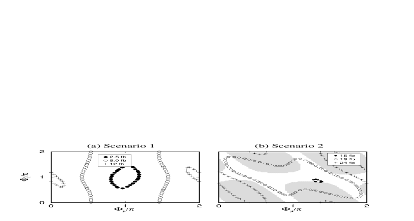
We present in Fig. 11 the contour plots for the total cross section on the plane of two CP–violating phases $\{\Phi_{\mu},\Phi_{1}\}$ in the two scenarios (a) ${\cal S}1$ and (b) ${\cal S}2$. In the scenario ${\cal S}1$ the branching fraction ${\cal B}(\tilde{\chi}^{-}_{1}\rightarrow\tilde{\chi}^{0}_{1}\,\ell^{-}\bar{\nu}_{\ell})$ is almost constant as shown in Fig. 10 so that the total tri–lepton cross section is mainly determined by ${\cal B}(\tilde{\chi}^{0}_{2}\rightarrow\tilde{\chi}^{0}_{1}\,\ell^{\prime+}\ell^{\prime-})$ and the production cross section $\sigma(p\bar{p}\rightarrow\tilde{\chi}^{-}_{1}\tilde{\chi}^{0}_{2})$. The total tri–lepton cross section is of the order of $1$ fb (10 fb) for the parameter sets ${\cal S}1$ (${\cal S}2$), respectively. However in the future Tevatron RUN-II experiments with the upgraded luminosity of the order of 2 fb-1 a handful of tri–lepton events can be produced. Note that the total cross section is sensitive to the CP-violating phases in the scenario ${\cal S}2$ and the cross section can be minimal for certain non–trivial values of the CP–violating phases. This property is mainly due to the fact that the branching fraction ${\cal B}(\tilde{\chi}^{-}_{1}\rightarrow\tilde{\chi}^{0}_{1}\,\ell^{-}\bar{\nu}_{\ell})$ exhibits a similar pattern as shown in Fig. 10. Therefore, depending on the size of the integrated luminosity the very existence of the minimum event rate and the simultaneous small mass splitting (See Fig. 4) for the non–trivial CP–violating phases reflect that the Tevatron bounds on $m_{\tilde{\chi}^{\pm}_{1}}$ and $m_{\tilde{\chi}^{0}_{2}}$ might be much smaller than those [27] ruled out in the context of SUGRA and GUT inspired SUSY models.

6.3 Dilepton invariant mass distributions

The final–state leptons of the neutralino decay $\tilde{\chi}^{0}_{2}\rightarrow\tilde{\chi}^{0}_{1}\,\ell^{\prime+}\ell^{\prime-}$ provides us with a very easily measurable kinematical observable; the dilepton invariant mass, $m_{\ell\ell}$. This Lorentz–invariant quantity can be precisely reconstructed by measuring the two lepton momenta, and it is nothing but the square root of the Mandelstam variable, $\sqrt{s^{\prime\prime}}$,

$\displaystyle m_{\ell\ell}=\sqrt{s^{\prime\prime}}=m_{\tilde{\chi}^{0}_{j}}\sqrt{x_{3}+x_{4}-1+r_{j1}}\,.$ (90)

Furthermore, the invariant mass distribution is independent of the specific production process for the parent neutralino $\tilde{\chi}^{0}_{2}$, because the invariant mass does not involve any angular variables describing the decays so that the polarization of the decaying neutralino does not affect the distribution.

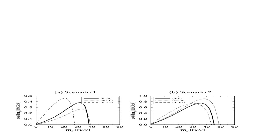
Figure 12 shows the dilepton invariant mass distribution in the scenarios (a) ${\cal S}1$ and (b) ${\cal S}2$. In principle, three dilepton combinations can be constructed out of the three charged leptons. But, the correct dilepton combination will have a sharp end point of its invariant mass distribution with a distinguishable peak in the dilepton invariant mass distribution. This allows one to experimentally determine the mass difference $\Delta_{m}=m_{\tilde{\chi}^{0}_{2}}-m_{\tilde{\chi}^{0}_{1}}$ with a good precision. Note that the position of the end points is strongly dependent on the CP–violating phases. It can provide us with the opportunity to probe the CP violating phases if all the other real parameters are known. As the gaugino masses vary significantly with the relevant CP violating phases, the distributions with respect to the kinematic variables like the energies and transverse momenta of the final–state leptons are strongly influenced by those CP–violating phases.

6.4 Lepton angular distribution in the laboratory frame

In a realistic experimental situation, it is necessary to isolate tri–lepton signal events by applying various selection cuts effectively to reduce the contaminations from all the background processes as much as possible. For that purpose, it is very important to fully understand the event topology of tri–lepton signal which depends on the polarizations of the chargino and neutralino at the intermediate stage. The full incorporation of the spin–correlations (81) involves a lot of correlated terms, which many Monte Carlo simulations [13] have simply neglected by including only the first un–correlated term in eq. (81). In this section, we take an easily–measurable kinematical variable, the scattering angle $\theta_{\ell}$ of the lepton from the chargino decay with respect to the proton beam direction and estimate the variation of the lepton angular distribution of the tri–lepton signal due to the spin–correlation effects.

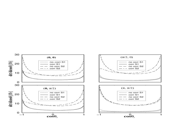
Figure 13 exhibits the lepton angular distribution of the tri–lepton signature for both the un–correlated case and the fully–correlated case for different phase combinations in both scenarios. Note that the correlated distribution can be different from the the un–correlated distribution around the forward and backward regions depending on the values of the CP–violating phases. In particular, the forward–backward asymmetry can be different in two cases. Therefore, even for this simple distribution it is important to take into account the spin correlations between production and decay fully to obtain the magnitude properly. Without any experimental cuts, such observables as the total tri–lepton event rate can be independent of whether the spin/angular correlations are taken into account or not. However, it might be inevitable to apply some efficient experimental cuts to suppress serious backgrounds. In that case the spin–correlations should be included.

6.5 CP–odd triple momentum products

So far we have concentrated mainly on the CP–even production–decay correlated observables which depend on the CP phases only indirectly. For direct measurements of the CP–violating phases one has to use CP–odd or T-odd observables. Some of such CP–odd (or T–odd) observables can be constructed by taking a triple product of any combination of the initial proton (or anti–proton) momentum and the three final lepton momenta. One typical example is the following triple momentum product (TMP):

$\displaystyle{\cal O}_{T}=\vec{p}_{{}_{\ell_{1}}}\cdot(\vec{p}_{{}_{\ell_{3}}}\times\vec{p}_{{}_{\ell_{4}}}),$ (91)

where $\ell_{1}=\ell^{-}$ of the chargino decay $\tilde{\chi}^{-}_{1}\rightarrow\tilde{\chi}^{0}_{1}\,\ell^{-}\bar{\nu}_{\ell}$, and $\ell_{3}=\ell^{\prime-}$, $\ell_{4}=\ell^{\prime+}$ of the neutralino decay $\tilde{\chi}^{0}_{2}\rightarrow\tilde{\chi}^{0}_{1}\,\ell^{\prime-}\ell^{\prime+}$. The observable (91) enables us to probe the CP–violating phases directly when neglecting the tiny particle decay widths. Similarly, the initial proton momentum and two final–state leptons allows us to construct additional T–odd observables:

$\displaystyle{\cal O}^{\ell\ell^{\prime}}_{T}=\vec{p}_{p}\cdot\left(\vec{p}_{\ell}\times\vec{p}_{\ell^{\prime}}\right)$ (92)

where $\{\ell,\ell^{\prime}\}$ is any combination of two momenta among the three final lepton momenta. In total, we have four independent TMPs; ${\cal O}_{T}$, ${\cal O}^{\ell_{1}\ell_{3}}_{T}$, ${\cal O}^{\ell_{1}\ell_{4}}_{T}$ and ${\cal O}^{\ell_{3}\ell_{4}}_{T}$.

In general, any of T–odd TMP can be given by a linear combination of the quartic charges $\{Q^{ij}_{4},C^{i}_{4},N^{j}_{4}\}$. We note that the same topological pattern of the contributing diagrams between the associated production and the chargino decay make $Q^{11}_{4}$ and $C^{1}_{4}$ correlated in size. Even before making any numerical estimate of the T–odd triple products, we can argue that their size is very small in the scenario ${\cal S}1$ with heavy sfermion masses. Firstly, the chargino and neutralino normal polarizations are very small in the scenario ${\cal S}1$ as shown in Sect. 4.4, implying small $Q^{12}_{4}$ and $C^{1}_{4}$. Secondly, with the negligible $t$– and $u$–channel slepton contributions, the remaining quartic charge $N_{4}$ of the neutralino $\tilde{\chi}_{2}^{0}$ simplifies to the expression

$\displaystyle N_{4}\approx\frac{|D_{Z}^{{}^{\prime\prime}}|^{2}}{c^{4}_{W}s^{4}_{W}}\,\left(s^{2}_{W}-\frac{1}{4}\right)\,\Im{\rm m}\left({\cal Z}^{2}_{21}\right)\,,$ (93)

which contains a very small numerical factor $(s^{2}_{W}-1/4)\sim-0.02$ [28]. Therefore, the quartic charge $N_{4}$ is also extremely suppressed in the scenario ${\cal S}1$. This simultaneous suppression of three quartic charges render all the TMPs strongly suppressed in the scenario ${\cal S}1$.

The three TMPS $\{{\cal O}_{T},\,{\cal O}^{\ell_{1}\ell_{3}}_{T},\,{\cal O}^{\ell_{1}\ell_{4}}_{T}\}$ involve both the chargino and neutralino leptonic decays, but the TMP ${\cal O}^{\ell_{3}\ell_{4}}$ involves only the neutralino leptonic decay. Therefore, one can have a large statistical gain by exploiting the observable ${\cal O}^{\ell_{3}\ell_{4}}_{T}$ in measuring the CP–violating phases. In this light, we consider only the observable ${\cal O}^{\ell_{3}\ell_{4}}_{T}$ to probe the CP–odd phases which are not excluded by the EDM constraints. Certainly, one needs to estimate all the possible systematic uncertainties in determining the reconstruction efficiency of the $\tilde{\chi}^{\pm}_{1}\tilde{\chi}^{0}_{2}$ mode. Nevertheless, let us take into account only the statistical errors including the hadronic decay modes of the chargino $\tilde{\chi}^{-}_{i}$ in the present work in which case the excluded region of $\{\Phi_{\mu},\Phi_{1}\}$ at the $N$ $\sigma$ level for a given integrated luminosity $\int{\cal L}\,{\rm d}t$ satisfies the inequality:

$\displaystyle\int{\cal L}\,{\rm d}t\geq\frac{N}{2}\frac{\langle({\cal O}^{\ell_{3}\ell_{4}}_{T})^{2}\rangle-\langle{\cal O}^{\ell_{3}\ell_{4}}_{T}\rangle^{2}}{|\langle{\cal O}^{\ell_{3}\ell_{4}}_{T}\rangle|^{2}\,\sigma_{tot}}\,,$ (94)

where $\sigma_{tot}=\sigma(p\bar{p}\rightarrow\tilde{\chi}^{-}_{1}\tilde{\chi}^{0}_{2})\,{\cal B}(\tilde{\chi}^{0}_{2}\rightarrow\tilde{\chi}^{0}_{1}\,\ell^{\prime+}\ell^{\prime-})$ and $\langle X\rangle\equiv\int X\,\frac{{\rm d}\sigma_{tot}}{{\rm d}\Phi}\,{\rm d}\Phi/\sigma_{tot}$ over the total phase space volume $\Phi$. The numerical factor 2 in the denominator is due to two possible combinations of the two final–state leptons; $(e^{-},e^{+})$ and $(\mu^{-},\mu^{+})$.

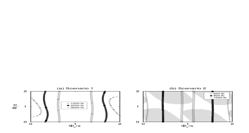
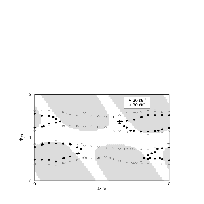
Figure 14 exhibits the region of the CP–violating phases $\Phi_{\mu}$ and $\Phi_{1}$ that is excluded by both the electron EDM constraints at 95% confidence level (shaded region) and by the T–odd observable ${\cal O}^{l_{3}l_{4}}_{T}$ at the 2–$\sigma$ level with an integrated luminosity of 20 fb-1 (filled circles) and 30 fb-1 (open circles) in the scenario ${\cal S}2$. Certainly, after incorporating all the systematic errors, the covered region should be reduced. Nevertheless, it might be useful to measure the T–odd observable at the upgraded Tevatron with an integrated luminosity ${\cal L}$ of the order of 30 ${\rm fb}^{-1}$ because the electron EDM and the T–odd TMP are complementary in constraining the CP–violating phases.

7 Conclusions

In this paper, we have investigated in detail the impact of the phases $\Phi_{\mu}$ and $\Phi_{1}$ on the SUSY tri–lepton signals at the Tevatron in the framework of MSSM with general CP phases but without generational mixing. The stringent constraints by the electron and neutron EDM on the CP phases have been also included in the discussion of the effects of the CP phases. For the sake of illustration, we have considered two exemplary scenarios for the relevant SUSY parameters; ${\cal S}1$ with very heavy first– and second–generation sfermions and ${\cal S}2$ with relatively light sfermions but a large $|\mu|$.

We have found that in both scenarios the CP–violating phases can have a significant impact on the production cross section and the partial leptonic branching fractions of the chargino $\tilde{\chi}^{\pm}_{1}$ and neutralino $\tilde{\chi}^{0}_{2}$. As a result, there may lead to a minimum rate of the tri–lepton signal for non–trivial CP phases. This implies that one should be careful when interpreting the chargino and neutralino mass limits derived under the assumption of vanishing phases, since the worst case is not (always) covered by just flipping the sign of $\mu$; rather it can occur from some non–trivial phases in between.

The production–decay spin correlations lead to several CP–even observables. We have studied the useful kinematical observables such as the dilepton invariant mass distribution, the angular distributions of the final–state leptons, and the T–odd (CP–odd) triple momentum products of the initial proton momentum and two final lepton momenta.

We have found that the the end point of the dilepton invariant mass distribution is very sensitive to the relevant CP–violating phases because of the strong dependence of the neutralino masses on the phases. Therefore, these distributions can be very useful in determining the phases once the other real SUSY parameters are known. The angular distributions of the final–state leptons taking into account the full spin/angular correlations can differ from the non–correlated ones by a few percents. Therefore, it will be sometimes necessary to consider the fully–correlated distributions in order to interpret experimental data properly.

It turned out to be difficult to investigate the CP–violating phases directly through the T–odd triple momentum products at the Tevatron with its upgraded luminosity of about 2 fb-1. But, we have found that a substantial region of the CP–violating phases may be explored through the triple momentum products with the luminosity of about 30 fb-1 as proposed for TeV33.

Acknowledgments

S.Y.C. and W.Y.S acknowledge financial support of the 1997 Sughak program of the Korea Research Foundation and M.G. acknowledges Alexander von Humboldt Stiftung foundation for financial help. H.S.S. is supported in part by the BK21 program.

References

  • [1] C. Giunti, C.W. Kim and U.W. Lee, Mod. Phys. Lett. A 6, (1991) 1745; U. Amaldi, W. de Boer and H. Fürstenau, Phys. Lett. B 260, 447 (1991); P. Langacker and M. Luo, Phys. Rev. D 44, 817 (1991); J. Ellis, S. Kelly and D.V. Nanopoulos, Phys. Lett. B 260, 131 (1991).
  • [2] For reviews, see H. Nilles, Phys. Rept. 110, 1 (1984); H.E. Haber and G.L. Kane, Phys. Rept. 117, 75 (1985); S. Martin, in Perspectives on Supersymmetry, edited by G.L. Kane, (World Scientific, Singapore, 1998).
  • [3] S. Dimopoulos and D. Sutter, Nucl. Phys. B 452 (1995) 496; H. Haber, Proceedings of the 5th International Conference on Supersymmetries in Physics (SUSY’97), May 1997, ed. M. Cvetić and P. Langacker, hep-ph/9709450.
  • [4] M. Brhlik and G.L. Kane, Phys. Lett. B 437, 331 (1998); S.Y. Choi, J.S. Shim, H.S. Song and W.Y. Song, ibid. B 449, 207 (1999).
  • [5] S.Y. Choi, M. Guchait, H.S. Song and W.Y. Song, Phys. Lett. B 483, 168 (2000); S.Y. Choi, H.S. Song and W.Y. Song, Phys. Rev. D 61, 075004 (2000).
  • [6] T. Falk and K.A. Olive, Phys. Lett. B 439, 71 (1998); T. Falk, A. Ferstl and K.A. Olive, Phys. Rev. D 59, 055009 (1999); ibid. D 60, 19904 (1999); T. Falk and K.A. Olive, Phys. Lett. B 375, 196 (1996); T. Falk, K.A. Olive and M. Srednicki, ibid. B 354, 99 (1995).
  • [7] A. Pilaftsis, Phys. Lett. B 435, 88 (1998); Phys. Rev. D 58, 096010 (1998); A. Pilaftsis and C.E.M. Wagner, Nucl. Phys. B 553, 3 (1999); D.A. Demir, Phys. Rev. D 60, 055006 (1999); S.Y. Choi, M. Drees and J.S. Lee, Phys. Lett. B 481, 57 (2000); M. Carena, J. Ellis, A. Pilaftsis and C.E.M. Wagner, hep–ph/0003180; B. Grzadkowski, J.F. Gunion and J. Kalinowski, Phys. Rev. D 60, 075011 (1999); G. Kane and L.-T. Wang, hep–ph/0003198; A. Pilaftsis, hep–ph/0003232.
  • [8] G.C. Branco, G.C. Cho, Y. Kizukuri and N. Oshimo, Phys. Lett. B 337, 316 (1994); Nucl. Phys. B449, 483 (1995); D.A. Demir, A. Masiero and O. Vives, Phys. Rev. Lett. 82, 2447 (1999); S.W. Baek and P. Ko, ibid., 83, 488 (1999).
  • [9] A. Masiero and L. Silvetrini, in Perspectives on Supersymmetry, edited by G.L. Kane, (World Scientific, Singapore, 1998); J. Ellis, S. Ferrara and D.V. Nanopoulos, Phys. Lett. B114, 231 (1982); W. Buchmüller and D. Wyler, ibid. B121, 321 (1983); J. Polchinsky and M.B. Wise, ibid. B125, 393 (1983); J.M. Gerard et al., Nucl. Phys. B253, 93 (1985); P. Nath, Phys. Rev. Lett. 66, 2565 (1991); R. Garisto, Nucl. Phys. B419, 279 (1994).
  • [10] T. Ibrahim and P. Nath, Phys. Lett. B 418, 98 (1998); Phys. Rev. D 57, 478 (1998), Erratum–ibid D 58, 019901 (1998); ibid. D 58, 111301 (1998), Erratum–ibid D 60, 099902 (1999); M. Brhlik, G.J. Good and G.L. Kane, ibid. D 59, 115004 (1999); S. Pokorski, J. Rosiek and C.A. Savoy, Nucl. Phys. B570, 81 (2000).
  • [11] Y. Kizukuri and N. Oshimo, Phys. Rev. D 45, 1806 (1992); 46, 3025 (1992).
  • [12] S. Dimopoulos and G.F. Giudice, Phy. Lett. B 357, 573 (1995); A. Cohen, D.B. Kaplan and A.E. Nelson, ibid. B 388, 599 (1996); A. Pomarol and D. Tommasini, Nucl. Phys. B466, 3 (1996). J. Bagger, J.L. Feng, N. Polonsky and R.-J. Zhang, Phys. Lett. B 473, 264 (2000); J.L. Feng, K.T. Matchev and T. Moroi, Phys. Rev. D 61, 075005 (2000); Phys. Rev. Lett. 84, 2322 (2000); J.L. Feng and T. Moroi, Phys. Rev. D 61, 095004 (2000); J. Bagger, J.L. Feng and N. Polonsky, Nucl. Phys. B563, 3 (1999).
  • [13] H. Baer et.al, Phys. Rev. D 61, 095007 (1999) and references therein.
  • [14] S. Weinberg, Phys. Rev. Lett. 63 2565 (1989); E. Braaten, C.S. Li and T.C. Yuan, ibid. 64 1709 (1990); J. Dai, H. Dykstra, S. Paban and D.A. Dicus, Phys. Lett. B 237.
  • [15] A. Manohar and H. Georgi, Nucl. Phys. B234, 189 (1984).
  • [16] R. Arnowitt, J. Lopez, and D.V. Nanopoulos, Phys. Rev. D 42, 2423 (1990); R. Arnowitt, M. Duff, and K. Stelle, ibid. D 43, 3085 (1991).
  • [17] D. Chang, W.-Y. Keung and A. Pilaftsis, Phys. Rev. Lett. 82, 900 (1999).
  • [18] H. Baer, C. Chen, M. Drees, F. Paige, and X. Tata, Phys. Rev. Lett. 79, 986 (1997); 80, 642(E) (1998); Phys. Rev. D 58, 975008 (1998); 59, 055014 (1999).
  • [19] Talk by T. Junk at the SUSY2K conference, CERN, June 26 - July 1, 2000.
  • [20] E.D. Commins, S.B. Ross, D. DeMille, and B.S. Regan, Phys. Rev. A 50, 2960 (1994); K. Abdullah et al., Phys. Rev. Lett. 65, 2347 (1990).
  • [21] M. Nojiri and Y. Yamada, Phys. Rev. D 60, 015006 (1999) and references therein.
  • [22] K. Hagiwara and D. Zeppenfeld, Nucl. Phys. B274, 1 (1986).
  • [23] L.M. Sehgal and P.M. Zerwas, Nucl. Phys. B183, 417 (1981).
  • [24] CTEQ Collaboration, H.L. Lai et al., Phys. Rev. D 51, 4763 (1995).
  • [25] W. Beenakker et. al. Phys. Rev. Lett. 83, 3780(1999); A. Djouadi and M. Spira, Phys. Rev. D 62, 014004 (2000).
  • [26] C. Bouchiat and L. Michel, Nucl. Phys. 5, 416 (1958); L. Michel, Suppl. Nuovo Cim. 14, 95 (1959); S.Y. Choi, Taeyeon Lee and H.S. Song, Phys. Rev. D 40, 2477 (1989).
  • [27] M. Carena et al., in Perspectives on Supersymmetry, edited by G.L. Kane, (World Scientific, Singapore, 1998); D0 Collaboration, B. Abbott et al., Phys. Rev. Lett. 80, 1591 (1998); CDF Collaboration, F. Abe et al., ibid. 80, 5275 (1998).
  • [28] C. Cao et al., Particle Data Group, Eur. Phys. J. C 3, 1 (1998).

Refer to caption


Figure 1: The Feynman diagrams contributing to the fermion EDMs and CEDMs in the MSSM; (a) one-loop chargino, neutralino and gluino diagrams and (b) two-loop top–Higgs or top quark–top squark–gluino diagrams.

Refer to caption

Figure 2: (a) the allowed range of the CP–violating phase $\Phi_{\mu}$ versus the higgsino mass parameter $|\mu|$ and (b) the allowed region of $\{\Phi_{\mu},\Phi_{1}\}$ against the electron (filled circles) and neutron (hollow circles) EDM constraints in the scenario ${\cal S}2$. The trilinear parameter $|A_{e}|$ is taken to be 1 TeV and its phase $\Phi_{A_{e}}$ is scanned over the full allowed range.

Refer to caption

Figure 3: The chargino and neutralino masses - (a) $m_{\tilde{\chi}^{-}_{1}}$, (b) $m_{\tilde{\chi}^{0}_{1}}$ and (c) $m_{\tilde{\chi}^{0}_{2}}$ - on the $\{\Phi_{\mu},\Phi_{1}\}$ plane in ${\cal S}1$ (upper frames) and ${\cal S}2$ (lower frames).

Refer to caption

Figure 4: The constraints on $\{\Phi_{\mu},\Phi_{1}\}$ by the measurements of the mass difference $\Delta_{m}=m_{\tilde{\chi}^{0}_{2}}-m_{\tilde{\chi}^{0}_{1}}$ for four different mean values of the mass difference $\Delta_{m}$ with the assumed uncertainty of 400 MeV in (a) ${\cal S}1$ and (b) ${\cal S}2$.

Refer to caption


Figure 5: Three mechanisms contributing to the parton–level production process $d\bar{u}\rightarrow\tilde{\chi}^{-}_{i}\tilde{\chi}^{0}_{j}$; the $s$–channel $W^{-}$ exchange, the $t$–channel $\tilde{u}_{L}$ exchange and the $u$–channel $\tilde{d}_{L}$ exchange.

Refer to caption


Figure 6: The differential production cross section ${\rm d}\sigma_{\rm prod}(p\bar{p}\rightarrow\tilde{\chi}^{-}_{1}\tilde{\chi}^{0}_{2}+X)/{\rm d}\cos\theta$ with respect to the cosine of the scattering angle, $\cos\theta$, in (a) ${\cal S}1$ and (b) ${\cal S}2$ for three different sets of $\{\Phi_{\mu},\Phi_{1}\}$.

Refer to caption

Figure 7: The production cross section $\sigma(p\bar{p}\rightarrow\tilde{\chi}^{-}_{1}\tilde{\chi}^{0}_{2}+X)$ on the $\{\Phi_{\mu},\Phi_{1}\}$ plane in (a) the scenario ${\cal S}1$ and (b) the scenario ${\cal S}2$.

Refer to caption

Figure 8: The normal polarization component of the neutralino $\tilde{\chi}^{0}_{2}$ with respect to the cosine of the scattering angle, $\cos\Theta$, in the process $d\bar{u}\rightarrow\tilde{\chi}^{-}_{1}\tilde{\chi}^{0}_{2}$ for four different combinations of $\{\Phi_{\mu},\Phi_{1}\}$ in (a) ${\cal S}1$ and (b) ${\cal S}2$. The parton–level c.m. energy is assumed to be 300 GeV for the sake of illustration.

Refer to caption


Figure 9: The three mechanisms contributing to (a) the chargino decay $\tilde{\chi}^{-}_{i}\rightarrow\tilde{\chi}^{0}_{1}\,\ell^{-}\bar{\nu}_{\ell}$ and (b) the neutralino decay $\tilde{\chi}^{0}_{j}\rightarrow\tilde{\chi}^{0}_{1}\,\ell^{\prime+}\ell^{\prime-}$. In both decays the exchanges of the charged and neutral Higgs bosons are neglected because they involve tiny lepton Yukawa couplings.

Refer to caption

Figure 10: The branching fractions ${\cal B}(\tilde{\chi}^{-}_{1}\rightarrow\tilde{\chi}^{0}_{1}\,\ell^{-}\bar{\nu}_{\ell})$ and ${\cal B}(\tilde{\chi}^{0}_{2}\rightarrow\tilde{\chi}^{0}_{1}\,\ell^{\prime+}\ell^{\prime-})$ for $\ell,\,\ell^{\prime}=e$ or $\mu$ on the $\{\Phi_{\mu},\Phi_{1}\}$ plane in the scenarios ${\cal S}1$ (upper part) and ${\cal S}2$ (lower part).

Refer to caption

Figure 11: The total cross section $\sigma(p\bar{p}\rightarrow 3\ell+{\rm X})$ of the tri–lepton signal on the $\{\Phi_{\mu},\Phi_{1}\}$ plane in the scenarios (a) ${\cal S}1$ and (b) ${\cal S}2$.

Refer to caption

Figure 12: The differential correlated cross section ${\rm d}\sigma_{\rm tot}/{\rm d}m_{\ell\ell}$ with respect to the invariant mass $m_{\ell\ell}$ of two leptons from the neutralino decay $\tilde{\chi}^{0}_{2}\rightarrow\tilde{\chi}^{0}_{1}\,\ell^{\prime+}\ell^{\prime-}$ for three different sets of $\{\Phi_{\mu},\Phi_{1}\}$ in the scenarios (a) ${\cal S}1$ and (b) ${\cal S}2$.

Refer to caption

Figure 13: The angular distribution of the charged lepton from the lightest chargino in the tri–lepton signal for the phases $\{\Phi_{\mu},\Phi_{1}\}$; $\{0,0\}$, $\{\pi/2,0\}$, $\{0,\pi/2\}$ and $\{\pi,\pi/2\}$ in the scenarios ${\cal S}1$ and ${\cal S}2$.

Refer to caption

Figure 14: The region of the CP–violating phases $\{\Phi_{\mu},\Phi_{1}\}$ excluded by the electron EDM measurements (black shadowed region) and probed by the T-odd TMP ${\cal O}^{l_{3}l_{4}}_{T}$ measurements with the integrated luminosity of 20 fb-1 (filled circles) and 30 fb-1 (open circles) at the 2–$\sigma$ level in the scenario ${\cal S}2$.